Solving the Non-Convexity Problem in Some
Shopping-Time and Human-Capital Models
y
Rubens Penha Cysne
zSeptember 10, 2004
Abstract
Several works in the shopping-time and in the human-capital lit-erature, due to the nonconcavity of the underlying Hamiltonian, use …rst-order conditions in dynamic optimization to characterize neces-sity, but not su¢ciency, in intertemporal problems. In this work I choose one paper in each one of these two areas and show that opti-mality can be characterized by means of a simple aplication of Arrow’s (1968) su¢ciency theorem.
1
Introduction
Several works in the economic literature, particularly in the shopping-time1 (e.g., Lucas (2000), Gillman, Siklos and Silver (1997), Cysne (2003), Cysne, Monteiro and Maldonado (2004))2 and in the human-capital literature (e.g. Uzawa (1965), Lucas (1988 and 1990), Chari, Jones and Manuelli (1995),
I am thnkful for comments of participants in workshops at the University of Chicago and at the Graduate School of Economics of the Getulio Vargas Foundation (EPGE/FGV). yKey Words: Arrow’s Su¢ciency Theorem, Optimal Control, Shopping-Time, Human Capital, Growth. JEL: E40, E50.
zProfessor at the Getulio Vargas Foundation Graduate School of Economics (EPGE/FGV) and, in 2004, a Visiting Scholar at the University of Chicago. Address: 5020 South Lake Shore Drive # 1402- N, Chicago IL, 60615 USA. E-mail:[email protected] 1As pointed out by Lucas (2000), nonconvexities in the shopping-time literature are related to the …xed costs of converting interest-bearing assets into cash (the costs of going to the bank in Baumol’s (1952) analysis).
Ladron-de-Guevara et al. (1999) and Kosempel (2001))3 use …rst-order con-ditions in dynamic optimization to characterize necessity, but not su¢ciency, in intertemporal problems. The reason, always either implicitly or explic-itly recognized by the authors, is that the non-concavity of the associated Hamiltonian does not allow for the use of Mangasarian’s (1966) well known su¢cient conditions in optimum control.
Mangasarian’s theorem states that if the Hamiltonian is (strictly) concave with respect to the control and the state variables, then the …rst-order con-ditions are also su¢cient for an interior (unique) optimum. The papers cited above are some examples in the economic literature in which such conditions are not obeyed.
Arrow’s (1968) theorem, though, generalizes Mangasarian’s result, and, as we shall see, is able to generate su¢ciency in some cases in which Man-gasarian’s result is not directly applicable. Arrow’s theorem requires another type of concavity. In words4, …rst, the Hamiltonian is maximized with re-spect to the control variables, for a given value of the costate variables. The optimum values of the control variables, as a function of the state variables and of the costate variable, are then substituted into the Hamiltonian. Call this new function (of the state and costate variables) the maximized Hamil-tonian. Arrow’s main result is that if this maximized Hamiltonian is (strictly) concave with respect to the state variable, for the given value of the costate functions, then the …rst order conditions characterize a (unique, concerning the state variable) optimum5.
Of course, if the Hamiltonian is concave with respect to both the state and control variables, then the maximized (with respect to the control variables) Hamiltonian will be concave in the state variables. But the reverse is not true. This is the reason why one says that Arrow’s theorem generalizes the Mangasarian’s su¢cient conditions.
The main purpose of this article is calling the attention to the fact, and exemplifying how, in some speci…c cases, an application of Arrow’s theorem can yield returns at very reasonable costs in terms of the required algebrisms. As a by-product of the analysis, a complementary insight into some papers of the shopping-time and human-capital literature (the ones used as examples) is also delivered.
3See equation (15) in Uzawa, equation (13) in Lucas (1988), equation (2.3) in Lucas (1990), equation (5) in Chari, Jones and Manuelli (1995), equation (2.4) in Ladron-de-Guevara et al. (1999) and equation (6) in Kosempel (2001, 2004).
4A formal version of Arrow’s theorem is presented in the next section.
Regarding the shopping-time literature, I concentrate the main analysis Cysne (2003). A solution to the problem of non-covexity found in Lucas (2000, section 5) follows the same general lines as those detailed here and is provided as a speci…c comment to that paper in Cysne (2004).
As it concerns the human-capital literature, I focus the analysis on Lucas (1988). The reason for concentrating on this paper is that its technology for accumulating human capital (equation (13) in Lucas (1988)) has been used by many other authors in the literature. This technology has actually been used before Lucas by Uzawa (1965)6. But it happens that Uzawa’s results can be obtained as a special case of Lucas’s modelling, when the utility is linear in consumption and there is not externality in production.
In the remaining of the paper, section 2 presents a formal version of Arrow’s theorem. In section 3 I exemplify the use and usefulness of the theorem within the shopping-time literature and, in section 4, within the human-capital literature. Section 5 concludes.
2
Arrow’s Theorem
Following Seierstad and Sydsater’s (1987, p. 107 and page 236), Arrow’s theorem, adapted to an in…nite horizon, reads as follows7:
Theorem 1 (Arrow’s Su¢ciency Theorem): Let (x(t); u(t)) (both contin-uously di¤erentiable) be a pair that satis…es the conditions (2) and (3) below, in the problem of …nding a piecewise-continuous control vector u(t) and an associated continuously-di¤erentiable state vector variable x(t); with x(t)
be-longing to a given open and convex set A 2 Rn for each t t0; de…ned on
the time interval [t0;1] , that maximizes:
Z 1
t0
f0(x(t); u(t); t)dt (1)
subject to the di¤erential equations:
_
xi(t) =fi(x(t); u(t); t); i= 1;2; :::; n (2)
6As well as by Rosen (1967), but in another context.
and to the conditions
x0i(t0) = x0i , i= 1;2; :::; n (3) xi(1) free; i = 1; :::; n
u(t) 2 U Rr:
Suppose, in addition, that x(t) belongs to (the open and convex set)A for all
t t0 and that, given the Hamiltonian function:
H(x(t); u(t); p(t); t) =f0(x(t); u(t); t) +
n X
i=1
pifi(x; u; t)
there exists a piecewise continuously-di¤erentiable function p(t) = (p1(t); :::; pn(t))
de…ned on [t0;1]such that H(x(t); u(t); p(t); t)exists and the following
con-ditions are satis…ed:
H(x(t); u(t); p(t); t) H(x(t); u(t); p(t); t); for all u2U, t 2[t0;1(4)]
_
pi(t) = Hxi(x(t); u(t); p(t); t); i= 1; :::; n (5) lim
t!1pi(xi(t) xi(t)) = 0 i= 1; :::; n (6)
H (x; p(t); t) =max
u2U H(x; u; p; t) exists and is a concave function ofx for all
t t0; then, (x(t); u(t)) solves problem (1)-(3) above.
3
An Application in a Shopping-Time Model
In this section I apply Arrow’s theorem to Cysne (2003).
Cysne (2003) considers an economy with n di¤erent assets performing monetary functions. Bonds (B) is the (n + 1)th asset. Bonds are used only as a store of value and pay the (endogenously determined) benchmark interest rate r: The monetary assets are represented by the n dimensional vector X = (X1; X2; :::; Xn); and their real quantities by the vector x =
(X1=P; X2=P; :::; Xn=P); P the price level: The real value of the sotck of bonds is b =B=P:Each asset x1; x2; :::; xn pays an interest rate r1; r2; :::; rn. Relatively to the benchmark rate, paid by bonds, the vector of opportunity costs reads u= (u1; u2; :::; un)= (r r1; r r2; :::; r rn):
With g > 0 denoting a discount factor and c consumption, households are assumed to maximize:
Z 1
The potential product (that available when the shopping time (s) is equal to zero) y is normalized to one. The household is endowed with one unit of time so that y+s= 1:Make rR = (r1 ; r2 ; :::; rn ) and denote by and h, respectively, the rate of in‡ation and the lump-sum transfers from households to the government. When maximizing (7), households face the budget constraint:
_
b+
n X
i=1
_
xi = 1 (c+s) h+ (r ) b+hrR; xi (8)
and the transacting-technology constraint:
c=G(x)s (9)
The monetary aggregator function G(x) is di¤erentiable, increasing in each one of the x variables, …rst degree homogeneous, and concave in x.
As in Lucas (2000), the utility function is assumed to be given by:
U(c) = c1 =(1 ); 6= 1; >0 (10)
U(c) = lnc( case = 1)
Below, we shall call the coe¢cient relative risk aversion8. The Hamiltonian for the problem reads:
H(s; G(x); b; ) = U(G(x)s)+ (1 (G(x)+1)s h+(r )b+
n X
j=1
(rj )xj)
(11) In order to apply Arrow’s theorem, consider s as the only control variable, and b and x as the state variables9. The above Hamiltonian clearly is not concave in these variables because of the term(G(x)+1)s:The maximization of (11) with respect to s leads (in any case) to:
s= 1
G(x)(
G(x) + 1
G(x) )
1= (12)
8Since there is no uncertainty in the model, should actually be called "the inverse of the elasticity of intertemporal substitution".
9Working with a = b+Pn
j=1xj as the only state variable (and s; and the xjs as
Substituting the expression of s into the Hamiltonian (11) leads to the max-imized Hamiltonian:
H (G(x); b; ) =
1 (
G(x)
(1 +G(x)))
(1 )= + (1 h+ (r )b+
n X
j=1
(rj )xj); ( #1)
H (G(x); b; ) = log G(x)
(1 +G(x)) + (1 1= h (r )b+
n X
j=1
(rj )xj)); ( = 1)
The next step in the application of the theorem is showing that the max-imized Hamiltonian is concave with respect to the state variables x and b:
Since the term in b is linear, the only variables we have to care about are those in the vector x:More precisely, those which are not in the linear term
Pn
j=1(rj )xj: The Hamiltonian is trivially concave in the case = 1 since
G(x) is concave and increasing in x and, given ( = U0(G1+(xG)s(x)G)(x) 0);
and taking G(x) as a variable, log (1+G(Gx)(x)) is a composite function of two monotone increasing concave functions. When 6= 1; note that the term
1 (
G(x) (1+G(x)))
(1 )= in the maximized Hamiltonian is concave in x (by the
same result that composite functions of increasing and concave functions are concave) provided that:
1
2 (13)
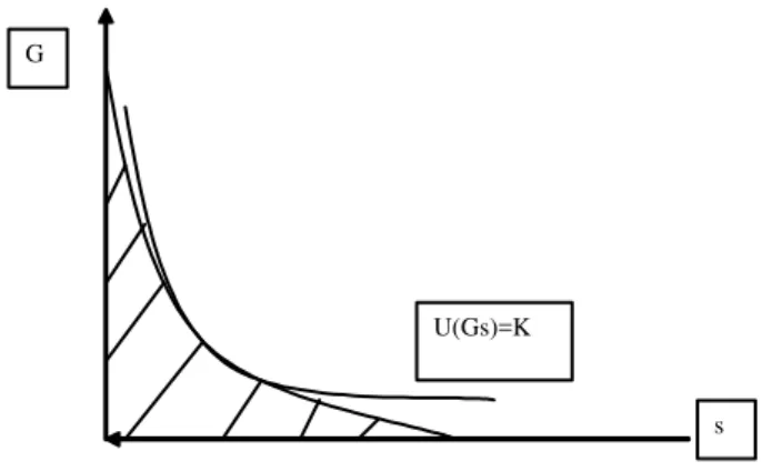
The extension of this reasoning to Cysne, Monteiro and Maldonado (2004) is straightfoward. The intuition10 for this result is presented in Figures 1 and 2 below.
(Please Insert Figures 1 and 2 here)
Figure 1 presents the case in which the coe¢cient of risk aversion is high enough. The feasible region of maximization is determined by the level curve of the term multiplying in (11). Even though this equation (through it’s isoquant) determines a non-convex feasible region in the(G(x); s)plane (the shadowed region in the …gures), if the curvature of the utility function is high enough the non-convexity poses no problem.
Figure 2 presents the problematic case, in which the …rst-order conditions (with equality) fail to characterize the optimum. This happens when the coe¢cient of risk aversion is not high enough.
4
An Application in a Human-Capital Model
In this section I will repeat the procedure of the last section, taking one paper in the human-capital literature and showing how it can bene…t from the application of Arrow’s theorem. For the reasons detailed in section 1, Lucas (1988) is a natural choice. In this paper preferences over consumption streams are (I omit the argument t of the functions in order to simplify the notation):
Z 1
0
e t N
1 (c
1 1); >0
and human capital (h) accumulates according to:
_
h=h(1 u)
Above, c (per-capita consumption) and u (the fraction of non-leisure time devoted to production) are control variables in the optimum path chosen by the representative consumer. N is the total number of workers and uN h is the e¤ective workforce used in the production of the consumption good.
WithK standing for the level of physical capital, the technology of goods production is:
N c+ _K =AK (uNh)1 h ; A >0; 0< <1; 0 (14)
The last term in the second member of equation (14), h ; stands for the externality of the level of human capital in the production of the consumption good. In the problem solved by the representative consumer (as opposed to that solved by a social planner), this term is taken as given.
The Hamiltonian in then given by (Lucas, 1988, p. 20):
H(K; h; 1; 2; c; u) =
N
1 (c
1 1) +
1 AK (uNh)1 h N c(15)
+ 2[ h(1 u)]
1 and 2are multiplier functions that give the marginal value of the state variables K and h, respectively, discounted back to time zero. Both 1 and
2; therefore, are nonnegative.
This Hamiltonian is clearly nonconcave in the control and state variables due to the term h(1 u): Denoting by Hx the derivative of H with respect
to (the generic) variable x:
Hu = 1AK ( Nh)1 (1 )h u 2 h
It also follows form the above equations that Hcc = 0 < 0; Huu < 0
and Huc = 0: Therefore, the Hamiltonian is strictly concave in (c; u): The
unique optimum values of these control variables can be found by making Hc =Hu = 0; in which case:
c= 1
1 (16)
u= ( 2
1AN1 (1 )
) 1Kh (17)
Substitute (16) and (17) in (15). The optimized (with respect to the control variables) Hamiltonian reads:
H (K; h; 1; 2) =
N
1 (
1
1 1) + 1KAN1 ( 2
1AN1 (1 )
) 1+ h
1
1 N + 2 h ( 2
1AN1 (1 )
) 1= h K
Since 0; the optimized Hamiltonian is concave in the state variable
K and h(though not strictly concave) only for = 0:
We conclude that, when there is no externality in the production of the consumption good due to the human-capital accumulation, the …rst-order conditions derived in the problem do represent a (not-necessarily-unique) optimum. Note that having > 0 is not so important in the theory de-veloped by Lucas (1988), since it predicts sustained growth whether or not the external e¤ect is present. The case = 0 (with = 1; linear utility) corresponds to Lucas’s version of Uzawa’s (1965) paper.
The case > 0 is not covered by Arrow’s theorem. Characterizing the optimum in this case requires other techniques.
5
Conclusion
References
[1] Arrow, K. J. (1968): "Applications of Control Theory to Economic Growth", in G. B. Dantzig and A. F. Veinott, Jr. eds., Mathematics of the decisions sciences (Providence, R. I. : American Mathematical Society).
[2] Arrow, K. and Kurz, (1970): "Public Investment, the Rate of Return and Optimal Fiscal Policy", The Johns Hopkins Press.’
[3] Baumol, W. J. (1952)"The Transactions Demand for Cash: An Inventory Theoretic Approach." QJE 66 :545-56.
[4] Chari, V., Larry E. Jones, and Rodolfo E. Manuelli (1995): "The Growth E¤ects of Monetary Policy", Federal Reserve Bank of Minneap-polis Quarterly Review Vol. 19 No. 4.
[5] Cysne, Rubens P. (2003): "Divisa Index, In‡ation and Welfare". Journal of Money, Credit and Banking, Vol 35, 2, 221-239
[6] Cysne, Rubens. P., Maldonado W. and Monteiro, Paulo K. (2004) "In‡a-tion and Income Inequality: A Shopping-Time Approach". Forthcoming, Journal of Development Economics.
[7] Cysne, Rubens P. (2004): " A Comment on "In‡ation and Welfare" ". Working Paper, EPGE/FGV and Department of Economics, The University of Chicago.
[8] Gillman, Max, Pierre Siklos and J.Lew Silver, (1997): "Money Velocity with Costly Credit ”, Journal of Economic Research, 2: 179-207. (The references in the text regard the draft prepared for the 1997 European Economic Association Meeting).
[9] Kosempel, S. (2001): "A Theory of Development and Long-Run Growth". Discussion Paper 2001-5, University of Guelph, Forthcoming, Journal of Economic Development.
[10] Ladron-deGuevara, A., S. Ortigeura and M. Santos (1999) "A Two-Sector Model of Endogenous Growth With Leisure." The Review of Economic Studies, Vol 66 n. 3 pp. 609-631.
[12] Lucas, R. E. Jr., (1990): "Supply Side Economics: An Analytical Re-view," Oxford Economic Papers 42:293-316.
[13] Lucas, R. E. Jr., (2000): "In‡ation and Welfare". Econometrica 68, No. 62 (March), 247-274.
[14] Mangasarian, O. L., (1966): "Su¢cient Conditions for the Optimal Con-trol of Nonlinear Systems, Siam Journal on ConCon-trol", IV, February, 139-152.
[15] Pontryagin, L. S.; Boltyanskii, V.; Gamkrelidze, R.; and Mischenko, E. 1962, "The Mathematical Theory of Optimal Process", New York and London, Interscience.
[16] Rosen, S. (1976): "A Theory of Life Earnings", Journal of Political Economy, Vol. 84, Part 2, 545-567.
[17] Seierstad, A. and Sydsaeter K., (1977): "Su¢cient Conditions in Op-timal Control Theory", International Economic Review, Vol. 18, No2,
June.
[18] _________________, (1987): "Optimal Control Theory With Economic Applications", North Holland.
U(Gs)=K G
s
Figure 1: Non-Problematic Case - Coe¢cient of Risk Aversion High Enough
U(Gs)=K G
s
! " #$$% &'(
) * + + , - . + , / , 0 1 ,2 3 +4 56
5 5 7 .5 7 5 5 ! " #$$% #% &'(
8 + 9 , 1 ,2 3 +4 56 1 : !
! " #$$% #; &'(
#$ + < +, +, + = > + , , 9 +. 9
9 , 1 ,2 3 +4 5 ! " #$$% &'(
# + + 9 , < , + + ?
@ ,A B 5 #$$; C &'(
## , + = , D + 9+, + 1
6 ? D 5 ( 3 5 7 5 #$$; #% &'(
#% < + +, + + + . + 9 D E 5 ?F 6
?" 3 5 6 1 ?1@5 7 5 #$$; # &'(
#; + .+ + +. G E 5 ?F 6 ?" 3 5 6 1
?1@5 7 5 #$$; #C &'(
# 5 " ( - ( 5! 35 5( - 5 1 357 & 75 5 , 5 35 , 3 6 5
5 6 ?" 3 5 7 5 #$$; &'(
#C 3 H 5 35 " 51 1 3 H3 B? 5 B ? IJ 6 ?" 3 5
7 5 #$$; 8 &'(
# 51 1 5 15 3 3575 1 2"51 ?" 1 (5 1 K &
5 ( B 3L 7 ? 3 6 B J 513 6 5 & 1 7 7 5
#$$; ; &'(
#) +. 9+ + = + >@5F5 :5 6 ?5!
3 5" I #$$; # &'(
#8 ,D + + = , +. 9 9 G , +,= + , + ,
?5! 3 5" 6 >@5F5 :5 I #$$; # &'(
%$ + < , + = A ? ( D5"6 ?5! 3 5" I
#$$; %C &'(
% > + + + 9 , +, + +M +, >
, 7 1 35 5 6 .5 7 5 11@5 5 I #$$; # &'(
%# . + 9, + G , 9+ , 9 : , ( B 4
3L 7 6 , 7 1 35 5 6 ' 15 32 5 7 3 I #$$; #
&'(
%; +0 , : B9 + P , + * I #$$; % &'(
% , + + :, +. +, , + > M
+ = 1 " 6 35 35 6 5( 5 3 I #$$; %8
&'(
%C Q9 , 9, + ? D 5 ( 3 5 I
#$$; C &'(
% 9, + < 9 + + = + =
:, 9 + ? D 5 ( 3 5 6 ?H 7 53 6 R ( B I #$$;
) &'(
%) +, + Q9 = + B , < . + 9
+, ? @ ,A I #$$; % &'(
%8 + , +* + S+, + , +* + M 8; #$$%
? @ ,A 6 ? , , 5" 5 I #$$; &'(
;$ + , + 9 + , ? 7 A ? @
,A 5 #$$; #C &'(
; 9 + + = 9+ +. = + ?5!
3 5" 6 >@5F5 :5 5 #$$; #% &'(
;# + = 9+ + + 9, = +, + , 9 , 9+
5 " , " 6 3 . 2 - B 6 , 15 5 " 53 5 #$$; # &'(
;% < + 9, T U + + + < V ? @ ,A 5
#$$; 8 &'(
;; , + + + 9 = , = , + , +
"? ? 6 W 5 #$$; $ &'(
; + = < +D + < D 51 , 7 1 356 5X? ! "
&
;C ,=, , + = + + + + = 51 , 7 1 356 5X?
! " &
; : + P , + * + + D =+ +
5 #$$; 8 &'(
;) 9 + + + + 9 9 +, Y 8C$ #$$$ZM ,
9, = , 7 1 35 5 6 "? ? 6
B? @ #$$; % &'(
;8 +, , , P , , + 9 9 * +
+ 9 * +N 9 * ' 5 ?(? 3 5 . " 6 B J
513 ' 15 32 5 7 3 B? @ #$$; #) &'(
$ + Q9 + , + +
, [ + + , + B J 513 6 1@ , ?3 5 B? @ #$$;
, + . +,= < + +, 75 35" 36 ?" 3 5
B? @ #$$; % &'(
# 9 , +. < = + 9+ M 9 + = >@5F5
:5 6 ?5! 3 5" B? @ #$$; %$ &'(
% : .+ < , + , 9+ .+ +. + .
5 5 ?F 6 5 . 33 5 6 ?" 3 5 B? @ #$$; ; &'(
; D 9 + , + .+ . + + ,
, , 3 6 ?1 B 3 5 B? @ #$$; %# &'(
++ +. + + 9 , 5 . 33 5 6 ?1 3 5
B? @ #$$; # &'(
C , , +\ , ,9 , 9 + N + .
S+, + 5 !6 , 7 1 35 5 B? @
#$$; % &'(
+ + + +, + Q9 =M +D 9. B , ,
? @ ,A ( 3 #$$; % &'(
) , , : + + + . , + < +
+, + +, ? @ ,A ( 3 #$$; # &'(
8 +, + Q9 =M +, + B , , ?
@ ,A ( 3 #$$; ) &'(
C$ < 9 +, + Q9 = = , 9
= + + 9+ = + ? @ ,A ( 3
#$$; # &'(
C + , + < + +, + Q9 = + 9+ = +
? @ ,A ( 3 #$$; ; &'(
C# . + Q9 9 , 9 + < ,
+ +Y , +.- , + Z ? @ ,A
( 3 #$$; $C &'(
C% , +] , 9 , 1 ,2 3 + 56
1 , : ! ( 3 #$$; ;$ &'(
C; + 9 Y 9 + Z ,. +. + + . + + ,=
3 . 2 B 3 " #$$; ; &'(
C + 9 , Y+ N + +^ 8
#$$%Z 1 ,2 3 + 56 1 , : ! 3 " #$$; %8 &'(
CC + + + +, + Q9 =M +. , Y ,
+.-B 9 + + , + , Z ? @ ,A 6 <5 W 6
? D 5 ( 3 5 3 " #$$; &'(
C +. + + , + : = + +. + 9 +