Hybrid inventory, gravimetry and altimetry (HIGA) mass balance product for Greenland and the Canadian Arctic

TCD

HIGA mass balance product for Greenland and the

Canadian Arctic

W. Colgan et al.

Title Page

Abstract Introduction

Conclusions References

Tables Figures

◭ ◮

◭ ◮

Back Close

Full Screen / Esc

Printer-friendly Version Interactive Discussion

Discussion

P

a

per

|

D

iscussion

P

a

per

|

Discussion

P

a

per

|

Discuss

ion

P

a

per

|

The Cryosphere Discuss., 8, 537–580, 2014 www.the-cryosphere-discuss.net/8/537/2014/ doi:10.5194/tcd-8-537-2014

© Author(s) 2014. CC Attribution 3.0 License.

Open Access

The Cryosphere

Discussions

This discussion paper is/has been under review for the journal The Cryosphere (TC). Please refer to the corresponding final paper in TC if available.

Hybrid inventory, gravimetry and altimetry

(HIGA) mass balance product for

Greenland and the Canadian Arctic

W. Colgan1,2, W. Abdalati2, M. Citterio1, B. Csatho3, X. Fettweis4, S. Luthcke5, G. Moholdt6, and M. Stober7

1

Marine Geology and Glaciology, Geological Survey of Denmark and Greenland, Copenhagen, Denmark

2

Cooperative Institute for Research in Environmental Sciences, University of Colorado, Boulder, CO, USA

3

Department of Geology, State University of New York, Bu_ffalo, NY, USA 4

Department of Geography, University of Liége, Liége, Belgium 5

Goddard Space Flight Center, National Aeronautics and Space Administration, Greenbelt, MD, USA

6

Scripps Institution of Oceanography, University of California, San Diego, CA, USA 7

Stuttgart University of Applied Sciences, Stuttgart, Germany

Received: 3 January 2014 – Accepted: 8 January 2014 – Published: 23 January 2014

Correspondence to: W. Colgan (wic@geus.dk)

TCD

HIGA mass balance product for Greenland and the

Canadian Arctic

W. Colgan et al.

Title Page

Abstract Introduction

Conclusions References

Tables Figures

◭ ◮

◭ ◮

Back Close

Full Screen / Esc

Printer-friendly Version Interactive Discussion

Discussion

P

a

per

|

D

iscussion

P

a

per

|

Discussion

P

a

per

|

Discuss

ion

P

a

per

Abstract

We present a novel inversion algorithm that generates a mass balance field that is simultaneously consistent with independent observations of glacier inventory de-rived from optical imagery, cryosphere-attributed mass changes dede-rived from satel-lite gravimetry, and ice surface elevation changes derived from airborne and satelsatel-lite

5

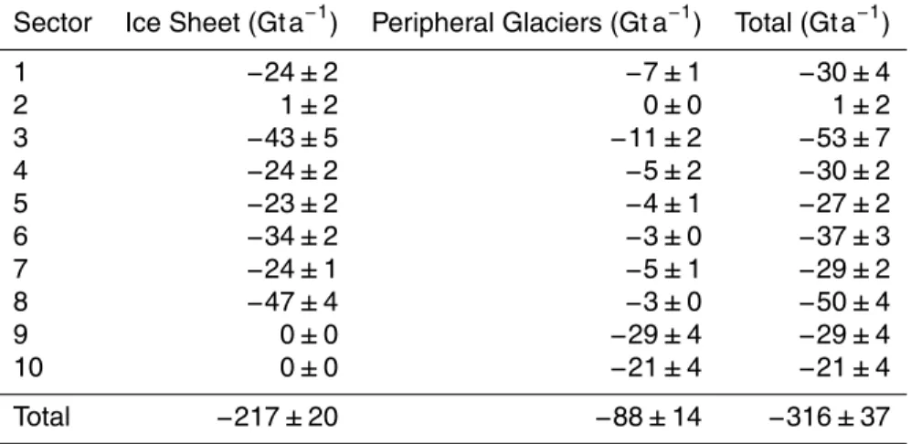
altimetry. We use this algorithm to assess mass balance across Greenland and the Canadian Arctic over the December 2003 to December 2010 period at 26 km resolu-tion. We assess a total mass loss of 316±37 Gt a−1 over Greenland and the Cana-dian Arctic, with 217±20 Gt a−1 being attributed to the Greenland Ice Sheet proper, and 38±6 Gt a−1and 50±8 Gt a−1being attributed to peripheral glaciers in Greenland

10

and the Canadian Arctic, respectively. These absolute values are dependent on the gravimetry-derived spherical harmonic representation we invert. Our attempt to vali-date local values of algorithm-inferred mass balance reveals a paucity of in situ ob-servations. At four sites, where direct comparison between algorithm-inferred and in situ mass balance is valid, we find an RMSD of 0.18 m WE a−1. Differencing

algorithm-15

inferred mass balance with previously modelled surface mass balance, in order to solve the ice dynamic portion of mass balance as a residual, allows the transient glacier con-tinuity equation to be spatially partitioned across Greenland.

1 Introduction

Greenland is presently the single largest cryospheric source of sea level rise,

contribut-20

ing 0.73 ± 0.08 mm a−1 of sea level rise during the 2005 to 2010 period (Shepherd et al., 2012). Greenland’s contribution to sea level rise is believed to have been ap-proximately equally divided between anomalies in meltwater runoffand iceberg calving during the 2000 to 2008 period (van den Broeke et al., 2009). Pursuing a process-level understanding of this contemporary partitioning of mass loss requires characterizing

25

TCD

HIGA mass balance product for Greenland and the

Canadian Arctic

W. Colgan et al.

Title Page

Abstract Introduction

Conclusions References

Tables Figures

◭ ◮

◭ ◮

Back Close

Full Screen / Esc

Printer-friendly Version Interactive Discussion

Discussion

P

a

per

|

D

iscussion

P

a

per

|

Discussion

P

a

per

|

Discuss

ion

P

a

per

|

modelled surface mass balance to be differenced from total mass balance in order to solve for the ice dynamic component of mass change through iceberg calving. Accu-rate knowledge of the contemporary partitioning of mass loss between meltwater runoff

and iceberg calving can serve as a key diagnostic modelling target, in order to improve confidence in subsequent prognostic model simulations.

5

Three methods are available for assessing mass balance at ice sheet scale: (i) input-output, (ii) volume change, and (iii) gravity change. The first approach, also known as the mass budget approach, differences ice discharge estimated near the grounding line of outlet glaciers from surface mass balance modelled over the ice sheet (e.g. Rignot et al., 2008). The second approach converts surface elevation changes observed by

10

repeat airborne or satellite altimetry into mass changes using an e_ffective density of change estimated through firn density modelling (e.g. Zwally et al., 2011). The third approach uses repeat satellite gravimetry observations and numerous geophysical for-ward models to assess absolute cryospheric mass changes (e.g. Velicogna and Wahr, 2005). Each method has unique advantages and disadvantages relative to the other

15

methods (Alley et al., 2007). While satellite altimetry characterizes the spatial vari-ability of mass changes at relatively high resolution, it relies on forward modelling of complex firn processes to produce absolute mass changes. Conversely, the absolute cryospheric mass changes observed by satellite gravimetry and isolated by forward models have relatively poor spatial resolution.

20

Here, we combine the two strengths of gravimetry and altimetry in order to refine absolute measurements of cryosphere-attributed mass change to relatively high spa-tial resolution. In this process, we overcome two complementary weaknesses: depen-dence on modelling complex firn processes as well as the fundamental spatial res-olution of satellite gravimetry. The mass balance field we derive through an iterative

25

TCD

HIGA mass balance product for Greenland and the

Canadian Arctic

W. Colgan et al.

Title Page

Abstract Introduction

Conclusions References

Tables Figures

◭ ◮

◭ ◮

Back Close

Full Screen / Esc

Printer-friendly Version Interactive Discussion

Discussion

P

a

per

|

D

iscussion

P

a

per

|

Discussion

P

a

per

|

Discuss

ion

P

a

per

this 2004 to 2010 mean annual mass balance field may offer the most spatially ac-curate direct assessment of the combined mass balance of both Greenland and the Canadian Arctic to date.

2 Method

2.1 Data

5

Our inversion algorithm requires three distinct pieces of input data: (i) fractional ice cov-erage derived from optical imagery, (ii) cryosphere-attributed mass changes derived from satellite gravimetry, and (iii) ice surface elevation changes derived from satel-lite altimetry. We compile each of these datasets over a common region of interest focused on Greenland and the Canadian Arctic (Fig. 1). Our time period of interest

10

follows the gravimetry comparison interval adopted by the ice sheet mass balance inter-comparison exercise (IMBIE): December 2003 to December 2010 (Shepherd et al., 2012). We assess mass balance in ten geographic sectors, eight in Greenland and two in the Canadian Arctic. The eight Greenland sectors are equivalent to the eight major ice sheet drainage systems delineated by Zwally et al. (2012), but have been

15

extended beyond the ice sheet margin to also encompass peripheral glaciers and ice caps. The two Canadian Arctic sectors are equivalent to those employed by Gardner et al. (2011). Shapefiles of these ten sector boundaries are available in the Supplement associated with this paper.

We calculated the fractional ice coverage within our study region by clipping

object-20

oriented glacier inventory polygons with a polygon fishnet matching the inversion grid. We then summed the glacierized area within each grid cell, and scaled to correct for projection-related area distortion. In Greenland, we summed peripheral glacier and ice sheet coverage separately. The Greenland glacier inventory data are derived from aerophotogrammetry with a polygon accuracy of 10 m (Citterio and Ahlstrøm, 2013).

25

connectiv-TCD

HIGA mass balance product for Greenland and the

Canadian Arctic

W. Colgan et al.

Title Page

Abstract Introduction

Conclusions References

Tables Figures

◭ ◮

◭ ◮

Back Close

Full Screen / Esc

Printer-friendly Version Interactive Discussion

Discussion

P

a

per

|

D

iscussion

P

a

per

|

Discussion

P

a

per

|

Discuss

ion

P

a

per

|

ity with the ice sheet proper as Greenland peripheral glaciers, while glaciers demon-strating “strong” connectivity with the ice sheet are classified as part of the Greenland Ice Sheet proper (cf. Rastner et al., 2012). The Canadian glacier inventory data are de-rived from the Randolph Glacier Inventory (RGI) version 2.0 (Arendt et al., 2012). We employ both the North and South Canadian Arctic (RGI regions 3 and 4), which are

5

primarily based on Landsat imagery with polygon accuracy of about 30 m. We also use the RGI to calculate fractional ice coverage over Svalbard and a small portion of Ice-land (RGI regions 6 and 7) in the far-field of our inversion domain. We take the glacier polygons in both the Citterio and Ahlstrøm (2013) and Arendt et al. (2012) inventories to be representative of ice coverage during the IMBIE period.

10

The gravimetry-derived cryospheric mass change product we employ is identical to that described in Colgan et al. (2013). This mascon solution is estimated directly from the formal reduction of Gravity Recovery and Climate Experiment (GRACE) K-band inter-satellite range rate (KBRR) data, processing the level 1B (L1B) data, including attitude and accelerometer data. Forward models for ocean tides and ocean mass

15

variations (GOT4.7/OMCT; Ray, 1999), atmospheric mass variations (ECMWF; Ray and Ponte, 2003), terrestrial water storage (GLDAS/Noah; Ek et al., 2003; Rodell et al., 2004) and glacial isostatic adjustment and little ice age correction (ICE-5G; Peltier, 2004) are employed in the L1B data processing in order to isolate land ice mass variations of interest (and, in the case of forward hydrology modeling, limiting

corre-20

lated residual signal contribution to the land ice solutions). Within Greenland, the trend in each of these corrections is<5 Gt a−1, and therefore small relative to the trend in cryospheric mass change (∼2 %). Complete details on these forward models and indi-vidual trend magnitudes are presented in Luthcke et al. (2013). Covariance constraints are applied by constraint region (e.g. Greenland Ice Sheet and oceans) in order to limit

25

TCD

HIGA mass balance product for Greenland and the

Canadian Arctic

W. Colgan et al.

Title Page

Abstract Introduction

Conclusions References

Tables Figures

◭ ◮

◭ ◮

Back Close

Full Screen / Esc

Printer-friendly Version Interactive Discussion

Discussion

P

a

per

|

D

iscussion

P

a

per

|

Discussion

P

a

per

|

Discuss

ion

P

a

per

Following L1B data reduction, the residual cryosphere-attributed linear mass change trend and 1σtrend error are calculated for each mascon time series and subsequently converted into equivalent spherical harmonics of degree and order 60 via a set of differential potential coefficients (“delta coefficients”) applied to the mean GRACE level 2 (L2) field (Chao et al., 1987; Luthcke et al., 2013). In comparison to relatively sharp

5

contrasts in mass change characteristic of mascon boundaries, the relatively smooth spatial gradients of spherical harmonics are better suited for the isotropic inversion filter we employ. The GRACE-derived cryosphere-attributed mass change trend we employ is calculated over the IMBIE GRACE comparison period (December 2003 to December 2010; Shepherd et al., 2012). We acknowledge that mascons ultimately

10

provide a better inversion target than mascon-derived spherical harmonics, but we note that a mascon inversion requires an anisotropic geometric filter, and thus represents a non-trivial extension of the isotropic inversion we present.

The satellite altimetry-derived estimates of ice surface elevation change we employ are primarily based on Ice, Cloud and land Elevation Satellite (ICESat) observations

15

from 2003 to 2009. In Greenland, 2 km spatial resolution surface elevation changes are derived from altimetry data following the approach of Schenk and Csatho (2012), which corrects for intermission biases, ground controls and glacial isostatic adjust-ment. Schenk and Csatho (2012) also incorporate airborne laser observations when and where available. In the Canadian Arctic, 2 km spatial resolution surface elevation

20

changes are derived from ICESat data following the method of Gardner et al. (2011; 2012), with corrections applied for Gaussian-centroid offset (Borsa et al., 2013). Both the Greenland and Canadian Arctic ICEsat observations have been corrected for detec-tor saturation (Fricker et al., 2005). Unlike in Greenland, however, ICESat data (release 633) in the Canadian Arctic are not supplemented by airborne altimetry observations.

25

cov-TCD

HIGA mass balance product for Greenland and the

Canadian Arctic

W. Colgan et al.

Title Page

Abstract Introduction

Conclusions References

Tables Figures

◭ ◮

◭ ◮

Back Close

Full Screen / Esc

Printer-friendly Version Interactive Discussion

Discussion

P

a

per

|

D

iscussion

P

a

per

|

Discussion

P

a

per

|

Discuss

ion

P

a

per

|

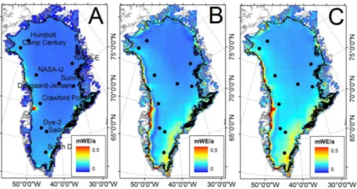
erage seldom approaches 100 %, an average of 77 values are used to calculate mean surface elevation change within a given grid cell (Fig. 2).

We take the 1σ standard deviation of all rate of surface elevation change observa-tions within a given grid cell as characteristic of the uncertainty in the mean rate of sur-face elevation change of that grid cell. We determine rate of sursur-face elevation change,

5

as well as this associated 1σ uncertainty, over the IMBIE ICESat comparison period: September 2003 to October 2009 (campaigns 2a to 2f; Shepherd et al., 2012). The IMBIE ICESat comparison period starts nine months after, and ends thirteen months before, the IMBIE GRACE comparison period (∼13 % shorter). We therefore assume that the spatial distribution of ice surface elevation changes observed during the

ICE-10

Sat comparison period are generally representative of the GRACE comparison period. As firn correction factors are highly spatially correlated, as well as data intensive and difficult to parameterize, we do not correct surface elevation changes for firn densi-fication (or firn air content; e.g. Li and Zwally, 2011). The inversion algorithm e_ff ec-tively uses altimetry-derived surface elevation changes to distinguish relative trends in

15

cryospheric mass changes between adjacent ice-covered nodes; absolute cryospheric mass change is ultimately constrained by the gravimetry-derived spherical harmonic solution we employ. Thus, in contrast to most conventional altimetry studies, the inver-sion algorithm we present does not require effective densities to be associated with rates of surface elevation change. Simply put, we use altimetry to guide the finer

res-20

olution fingerprint of mass balance underlying a coarser resolution spherical harmonic solution of absolute mass change.

2.2 Algorithm

While the inversion algorithm presented by Colgan et al. (2013) had a spatial resolution of 26 km, this resolution was acknowledged as “nominal” given that specific mass

bal-25

ca-TCD

HIGA mass balance product for Greenland and the

Canadian Arctic

W. Colgan et al.

Title Page

Abstract Introduction

Conclusions References

Tables Figures

◭ ◮

◭ ◮

Back Close

Full Screen / Esc

Printer-friendly Version Interactive Discussion

Discussion

P

a

per

|

D

iscussion

P

a

per

|

Discussion

P

a

per

|

Discuss

ion

P

a

per

pable of constraining cryosphere-attributed mass changes to within ice-covered areas, and was not capable of distinguishing spatial heterogeneity in specific mass balance between adjacent ice containing nodes. The need for further independent information, capable of distinguishing different specific mass balances at adjacent ice-containing nodes, was identified in order to achieve “actual” 26 km resolution. The algorithm we

5

present below addresses this need, by introducing additional information in the form of altimetry-derived ice surface elevation change rate. This additional information per-mits different specific mass balances to be assigned at adjacent ice-containing nodes within irregularly-shaped ice-covered areas. The ultimate hybrid mass balance prod-uct derived from this inversion is consistent with fractional ice coverage,

cryosphere-10

attributed mass changes derived from satellite gravimetry, and ice surface elevation changes derived from altimetry.

In Colgan et al. (2013), gravimetry data are refined by introducing additional informa-tion in the form of fracinforma-tional ice coverage through a Gauss–Seidel-type iterative update of a higher resolution (26 km) mass balance field ( ˙m), according to:

15

˙

mk_{i j}+1₌m˙_{i j}k _{+ ∆}k_{i j}R_{i j}kF_{i j} (1)

wherekdenotes a given iteration andijare node indices in Cartesian coordinates. The iterative update term is the product of three terms: the difference between a Gaussian smoothed version of ˙m_{i j} and the input GRACE-derived spherical harmonic solution

20

(∆ki j), a random number from a uniform distribution between 0 and 1, which serves as a stochastic source (R_{i j}k), and finally independent information in the form of fractional ice coverage (F_{i j}). The first two of these terms vary by both iteration and node, whereas the latter only varies by node. A given simulation is initialized with a random ˙m_{i j} field, and then iteratively updated until convergence within a prescribed tolerance. In Monte

25

TCD

HIGA mass balance product for Greenland and the

Canadian Arctic

W. Colgan et al.

Title Page

Abstract Introduction

Conclusions References

Tables Figures

◭ ◮

◭ ◮

Back Close

Full Screen / Esc

Printer-friendly Version Interactive Discussion

Discussion

P

a

per

|

D

iscussion

P

a

per

|

Discussion

P

a

per

|

Discuss

ion

P

a

per

|

In this study, we introduce further independent information, observed ice surface elevation change rate, by adopting a successive over relaxation (SOR)-type parameter (ω_{i j}) into the iterative update term (Kincaid, 2004):

˙

mk_{i j}+1₌m˙k_{i j+ ∆}k_{i j}R_{i j}kF_{i j}ω_{i j} (2)

5

Whenω >1, SOR can accelerate the iterative convergence of a system of equations that approach their solution asymptotically, achieving substantial computational effi -ciency. In contrast, when ω <1, successive under relaxation can impart stability on the iterative convergence of potentially oscillatory systems of equations. Implement-ing a spatially variableω_{i j}, rather than a scalarω, across the inversion domain permits

10

inverted mass changes to be preferentially weighted to nodes with relatively highω val-ues, in comparison to adjacent nodes with relatively lowωvalues. As satellite altimetry is capable of resolving localized mass loss that results from outlet glacier accelera-tion (e.g. Zwally et al., 2011), altimetry-derived observaaccelera-tions of ice surface elevaaccelera-tion change rate provide a logical source of independent information for distinguishing

be-15

tween different specific mass balances at adjacent ice-containing nodes. Informingω_{i j} with observations of ice surface elevation change rate allows cryosphere-attributed mass changes to be spatially distributed in a fashion that is consistent with ice surface elevation changes.

We generate a first-order spatially variableω_{i j} field from observed ice surface

ele-20

vation change rates according to:

ω_{i j=}

˙ z_{i j}

z˙_{i j}

(3)

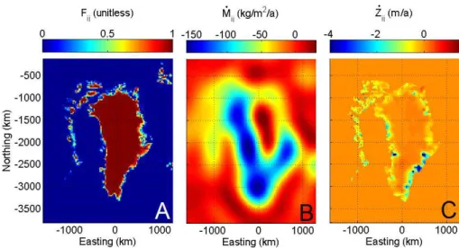
where ˙z_{i j} is altimetry-derived ice surface elevation change rate. This essentially com-putesω_{i j} as absolute normalized ice surface elevation change rate (Fig. 3); at a given

25

TCD

HIGA mass balance product for Greenland and the

Canadian Arctic

W. Colgan et al.

Title Page

Abstract Introduction

Conclusions References

Tables Figures

◭ ◮

◭ ◮

Back Close

Full Screen / Esc

Printer-friendly Version Interactive Discussion

Discussion

P

a

per

|

D

iscussion

P

a

per

|

Discussion

P

a

per

|

Discuss

ion

P

a

per

all absolute ice surface elevation change rates across the ten sectors of interest within the inversion domain. We evaluate this SOR-typeω_{i j} parameter at all ice-containing nodes within the inversion domain. We subsequently constrain extreme values ofω_{i j}. At nodes where calculatedω_{i j}<1, we prescribeω_{i j=}1 to prevent successive under relaxation. At the<0.01 % of nodes where calculatedω_{i j} >10, we prescribeω_{i j=}10.

5

These constraints allow the ω_{i j} parameter representing relative differences in ice surface elevation change to range over an order-of-magnitude across ice-containing nodes, while still maintaining numerical stability. For example, ten times more mass change would be attributed to a node withω₌10 than a neighboring node withω₌1. Spatial gradients inωacknowledge the reality that specific mass balance typically

de-10

creases to a minimum at the periphery of an ice mass. We similarly calculate uncer-tainty in this SOR-type parameter (δω_{i j}) as:

δω_{i j=}

σz˙_{i j}

z˙_{i j}

+ε

ω_{i j} (4)

whereσz˙_{i j} is the 1σ standard deviation of all observed ice surface elevation change

15

rates within node ij, and ε is a small number (taken here as 0.1 m a−1) to maintain numerical stability where ˙z_{i j→} 0. This essentially assumes that local uncertainty in ω_{i j} is directly proportional to local uncertainty in ice surface elevation change rate. In each simulation ω_{i j} is locally perturbed by the addition of δω_{i j}·R_{i j}, where R_{i j} is a random number array that varies by node in each simulation.

20

Following Colgan et al. (2013), we invert a 1000 simulation ensemble of GRACE-derived cryosphere-attribute rates of mass change. In each simulation within the ensemble, the best estimate of the GRACE-derived spherical harmonic representa-tion ( ˙MG) is randomly perturbed within its associated error (δM˙G), to yield a unique

˙

MG₊δM˙Ginput field. A given Monte Carlo simulation is initialized with a spatially

vari-25

able ˙m_{i j} field comprised of an array of random numbers uniformly distributed between

TCD

HIGA mass balance product for Greenland and the

Canadian Arctic

W. Colgan et al.

Title Page

Abstract Introduction

Conclusions References

Tables Figures

◭ ◮

◭ ◮

Back Close

Full Screen / Esc

Printer-friendly Version Interactive Discussion

Discussion

P

a

per

|

D

iscussion

P

a

per

|

Discussion

P

a

per

|

Discuss

ion

P

a

per

|

initial ˙m_{i j} field varies over the same order of magnitude as the anticipated final ˙m_{i j} field, and thus minimizes hysteresis resulting from prescribed initial conditions. Begin-ning with the initial condition, the higher resolution (26 km) mass balance field ( ˙m) is iteratively updated, substituting Eq. (2) (above) for Eq. (4) in Colgan et al. (2013), until convergence. In each iteration of each simulation the difference between the input ˙MG

5

and the Gaussian-smoothed ˙mfield ( ˙M) is randomly perturbed according to∆ki jR k i j in Eq. (2). We adopt the convergence parameter and isotropic Gaussian scaling length determined by previous sensitivity analysis, 0.1 Gt a−1 and 200 km, respectively (Col-gan et al., 2013). To summarize the multiple sources of stochasticity in the algorithm, random numbers are used to: (i) globally perturb the input GRACE-derived spherical

10

harmonic within its associated uncertainty in each simulation, (ii) locally perturb the SOR-type introduction of surface elevation change data in each simulation, and (iii) locally perturb the update term in each iteration. This ensures that inferred mass bal-ance is not required to be spatially correlated (e.g. subject to a covaribal-ance matrix), and enhances the algorithm’s ability to efficiently explore the infinite number of possible

15

solutions (e.g. Colgan et al., 2012).

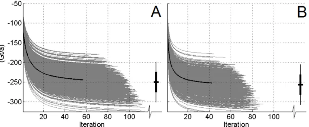
Implementation of this SOR-type convergence acceleration, through the introduction of an altimetry-informed ω_{i j} field as described by Eqs. (3) and (4), does accelerate convergence over the comparatively implicit ω₌1 approach of Colgan et al. (2013). A consequent decrease in the number of iterations required to reach convergence

20

translates into an ∼28 % gain in computational efficiency (Fig. 4). On high memory nodes of the University of Colorado Janus Supercomputer, a 2.8 GHz core with 12 GB of RAM solves the above system of equations with spatially variableωto convergence in 131±17 processor seconds (cf. 181±17 processor seconds in anω₌1 approach; Colgan et al., 2013). Further numerical gains in computational efficiency, which would

25

TCD

HIGA mass balance product for Greenland and the

Canadian Arctic

W. Colgan et al.

Title Page

Abstract Introduction

Conclusions References

Tables Figures

◭ ◮

◭ ◮

Back Close

Full Screen / Esc

Printer-friendly Version Interactive Discussion

Discussion

P

a

per

|

D

iscussion

P

a

per

|

Discussion

P

a

per

|

Discuss

ion

P

a

per

implementation of irregularly spaced grid systems, may offer the possibility to reduce the number of computation nodes by an order of magnitude (e.g. Bohlen and Saenger, 2006).

2.3 Boundaries

The inversion domain we employ is identical to that of Colgan et al. (2013). In the

5

US National Snow and Ice Data Center (NSIDC) polar stereographic projection, the inversion domain extends from−1625 km in the west to 1300 km in the east, and from

−125 km in the north to −3800 km in the south (Fig. 1). We employ a uniform grid spacing of 26 km, which results in 113 computational nodes along the Easting axis and 142 computational nodes along the Northing axis, for a total of 16 046 computational

10

nodes within the model domain. This grid spacing resolution is the highest resolution that allows the isotropic Gaussian filter node-specific dimensionless weighting values to be stored as a single three dimensional array of 113×142×16 046 elements on the per processor RAM available on the University of Colorado’s Janus Supercomputer. The polar stereographic projection inherently introduces increasing distortion away from its

15

central meridian (45◦W) and parallel (70◦N), which influences area calculations. We compensate for area distortion by calculating the true area of each individual node across the domain (A_{i j}). The true areas of ice-containing nodes vary between 24.52 and 27.52km2over the domain.

By employing a spherical harmonic representation of cryosphere-attributed mass

20

change ( ˙MG), the mass balances associated with non-ice containing nodes are the-oretically negligible (e.g. ˙m₌0 kg m−2a−1 where F ₌0). Practically, however, mass balances at non-ice containing nodes are not truly zero, but rather within uncertainty of zero (e.g. ˙m≈ 0 kg m−2a−1 where F ₌0). Following a sensitivity study by Col-gan et al. (2013), we prescribe a non-ice containing node absolute threshold ( ˙m_max)

25

of 15 kg m−2a−1. Simply put, this permits the inversion to assign between −15 and

TCD

HIGA mass balance product for Greenland and the

Canadian Arctic

W. Colgan et al.

Title Page

Abstract Introduction

Conclusions References

Tables Figures

◭ ◮

◭ ◮

Back Close

Full Screen / Esc

Printer-friendly Version Interactive Discussion

Discussion

P

a

per

|

D

iscussion

P

a

per

|

Discussion

P

a

per

|

Discuss

ion

P

a

per

|

uncertainty at non-ice containing nodes acknowledged by this boundary condition is representative of the level of uncertainty typically assessed for GRACE-derived cryosphere-attributed spherical harmonic solutions (e.g. Velicogna and Wahr, 2005; Longuevergne et al., 2010), and an order of magnitude less than the ˙m_{i j} values in-ferred by the inversion at adjacent ice-containing nodes. This boundary condition is

5

implemented at non-ice containing nodes according to a Heaviside, or logic, function invoked to appropriately modify Eq. (2) where F ₌0 (Eqs. 6 and 7 in Colgan et al., 2013).

3 Results

In comparison to the gravimetry-inversion mass balance product presented by Colgan

10

et al. (2013), which does not include altimetry-derived information on the relative ice surface elevation changes at adjacent nodes, the HIGA mass balance product assigns more mass loss at Greenland tidewater outlet glaciers, where relatively rapid dynamic drawdown is occurring, which is offset by less mass loss assigned further inland on the ice sheet (Fig. 5). This effectively results in a higher mass balance gradient with

dis-15

tance inland or elevation. Changes in specific mass balance between these two inver-sion approaches are negligible in both the ice sheet interior, where relative differences in surface elevation changes between adjacent nodes become small, and at non-ice containing nodes, where mass changes are constrained by boundary conditions. As the HIGA mass balance product assigns mass balance as proportional to relative

pe-20

riod trends in ice surface elevation rate, it yields a spatially heterogeneous specific mass balance field (i.e.per unit ice area), rather than one with gentle spatial gradients across ice-covered areas (cf. Fig. 13 of Colgan et al., 2013). Given the ability of an it-erative inversion to constrain GRACE-derived mass changes within irregularly-shaped ice-covered areas, and the inclusion of altimetry-derived surface elevation changes to

25

TCD

HIGA mass balance product for Greenland and the

Canadian Arctic

W. Colgan et al.

Title Page

Abstract Introduction

Conclusions References

Tables Figures

◭ ◮

◭ ◮

Back Close

Full Screen / Esc

Printer-friendly Version Interactive Discussion

Discussion

P

a

per

|

D

iscussion

P

a

per

|

Discussion

P

a

per

|

Discuss

ion

P

a

per

ensemble spread (Fig. 6). In Sect. 4.1, we attempt to validate HIGA ˙mvalues against in situ ˙mobservations. We note that the estimates of cryosphere-attributed mass change we present are dependent on the GRACE-derived spherical harmonic representation employed as algorithm input.

Over the IMBIE period, the HIGA inversion suggests that the Greenland Ice Sheet

5

proper was responsible for 217±20 Gt a−1 of mass loss (cf. 218±20 Gt a−1; Colgan et al., 2013). This is significantly less (∼17 %) than the ice sheet mass loss assessed by the IMBIE (263±30 Gt a−1; Shepherd et al., 2012). We note, however, that the IM-BIE grouped both peripheral glaciers and the ice sheet proper into a single Greenland mass loss value. Accounting for the additional mass loss of 38±6 Gt a−1 that we

at-10

tribute to Greenland peripheral glaciers over the period, brings our estimates of total Greenland mass loss within error of the IMBIE value (Table 1). The peripheral glacier mass loss of 50±8 Gt a−1that we attribute to the Canadian Arctic (Sectors 9 and 10) is greater than the analogous 33±22 Gt a−1 over the March 2003 to February 2010 period assessed by Schrama and Wouters (2011) using gravimetry, and less than the

15

reconciled altimetry and gravimetry estimate of 60±8 Gt a−1over the October 2003 to October 2009 period assessed by Gardner et al. (2013). We note that our Canadian Arctic mass loss estimate is within overlapping uncertainty of both these previously published values. Spatially variable tuning of the SOR-typeω_{i j} parameter may provide a means to reduce spatial discrepancies, but we elect to maintain our HIGA product as

20

completely untuned and consistent with Greenland IMBIE results.

Of the ten geographic sectors we examine across Greenland and the Canadian Arctic, only one (Sector 2 in Northeast Greenland) is within error of zero balance. The remaining nine sectors are in negative balance, resulting in a total ice loss of 316±37 Gt a−1across the study area over the IMBIE period. Peripheral glaciers in both

25

North-TCD

HIGA mass balance product for Greenland and the

Canadian Arctic

W. Colgan et al.

Title Page

Abstract Introduction

Conclusions References

Tables Figures

◭ ◮

◭ ◮

Back Close

Full Screen / Esc

Printer-friendly Version Interactive Discussion

Discussion

P

a

per

|

D

iscussion

P

a

per

|

Discussion

P

a

per

|

Discuss

ion

P

a

per

|

east Greenland. Mass loss from the ice sheet proper is greatest in Sectors 8 (Northwest Greenland) and 3 (East Greenland), where large tidewater glaciers are present, and least in Sector 1 (North Greenland), which is predominately land terminating. We note that while Sector 6 (Southwest Greenland) has relatively few tidewater glaciers, it has a greater mass loss than comparably-sized Sector 4 (Southeast Greenland) and

Jakob-5

shavn (Sector 7), both of which have appreciable numbers of tidewater glaciers. HIGA specific ˙mvalues (i.e. per unit ice area) reach a minimum of−4.2 m WE a−1 near the terminus of Jakobshavn Isbrae, and a maximum of 0.9 m WE a−1on the southern tip of Baffin Island. Following Colgan et al. (2013), we attribute this pocket of anomalous pos-itive values on Baffin Island to the inability of the inversion to satisfy anomalously high

10

oceanic mass gain within the parameter space we employ (e.g. characteristic Gaus-sian filter length scale and absolute threshold of non-ice containing nodes). This may reflect unidentified oceanic mass changes that are not captured in the forward ocean model used to isolate cryospheric mass loss, and note that gravimetry signal leakage is greatest where cryospheric mascons are surrounded by non-cryospheric mascons

15

on three sides.

4 Discussion

4.1 Comparison with in situ observations

Here, we compare local HIGA ˙mvalues with all available in situ ˙mobservations within our inversion domain. We believe this is the first time a GRACE-derived product has

20

been directly compared with point measurements of mass balance. We consider in situ ˙m measurements made via three techniques: (i) the “coffee can” approach, (ii) the surface mass balance and strain network method and (iii) repeat geodetic sur-vey with volume-to-mass conversion. The “coffee can” method, pioneered by Hamilton et al. (1998) and named after co_ffee cans deployed in boreholes, calculates change in

25

TCD

HIGA mass balance product for Greenland and the

Canadian Arctic

W. Colgan et al.

Title Page

Abstract Introduction

Conclusions References

Tables Figures

◭ ◮

◭ ◮

Back Close

Full Screen / Esc

Printer-friendly Version Interactive Discussion

Discussion

P

a

per

|

D

iscussion

P

a

per

|

Discussion

P

a

per

|

Discuss

ion

P

a

per

ice velocity, and a correction for subtle downslope movement of the coffee can during the measurement period. The unique aspect of this approach is correcting observed snow surface vertical velocity with a direct measurement of the rate of firn densification, in order to isolate vertical ice velocity at the firn–ice interface. Firn densification rate is assessed through repeat measure of the distance between a coffee can anchored at

5

depth and a given annual surface above (Hamilton et al., 1998). Coffee can-derived ˙m observations have been made at several sites on the Greenland Ice Sheet, as well as on the Devon Ice Cap (Hamilton and Whillans, 2002; Burgess et al., 2008). As ˙m is essentially derived by differencing long term ice dynamics and long term surface mass balance, the resultant ˙mvalues reflect mass balance for the past several decades

lead-10

ing up to the measurement period. Therefore, co_ffee can-derived ˙mvalues should only be compared to HIGA-inferred ˙mvalues with the knowledge that the latter reflects the 2004 to 2010 IMBIE period, while the former reflects a longer multi-decadal period.

The second method uses measurements of surface strain and surface mass balance to derives in situ ˙mby differencing long term ice dynamics and long term surface mass

15

balance. Rather than attempting to measure a densification-corrected vertical ice ve-locity, however, this approach relies on combining observations of local strain rates, both parallel and perpendicular to ice flow, with knowledge of ice thickness in order to assess vertical ice velocity via mass continuity (Reeh and Gundestrup, 1985; Burgess and Sharp, 2008). Thus, similar to the co_ffee can method, strain-derived ˙mvalues are

20

not directly comparable to HIGA values, as they reflect mean mass balance over the past several decades, rather the precise 2004 to 2010 IMBIE period. Within our inver-sion domain, strain-derived ˙m values are available at Dye-3 and the Devon Ice Cap (Reeh and Gundestrup, 1985; Burgess and Sharp, 2008). Although not directly com-parable, we still include both coffee can and strain-derived multi-decadal ˙m values in

25

our validation assessment, if only to demonstrate that 26 km spatial resolution HIGA ˙m values are reasonable.

TCD

HIGA mass balance product for Greenland and the

Canadian Arctic

W. Colgan et al.

Title Page

Abstract Introduction

Conclusions References

Tables Figures

◭ ◮

◭ ◮

Back Close

Full Screen / Esc

Printer-friendly Version Interactive Discussion

Discussion

P

a

per

|

D

iscussion

P

a

per

|

Discussion

P

a

per

|

Discuss

ion

P

a

per

|

mass balance (Stober et al., 2013). Unlike the other two in situ ˙m methods, neither long term ice dynamic nor long term surface mass balance are invoked in the geodetic method, which means that HIGA-inferred ˙mvalues are directly comparable to geodetic-derived ˙m values observed over the same period. Geodetic-derived ˙m values have been observed over the IMBIE period, or within a few years of the IMBIE period, at

5

both Swiss Camp and the Ohio State University (OSU) clusters in Greenland (Jezek, 2011; Stober et al., 2013). In the ablation region, where geodetic measurements are made on snow-free (bare) ice, the effective density of change can be assumed as the density of ice (e.g. Swiss Camp). In the accumulation region, where a snow pack or firn column exists, observations of surface elevation must be accompanied by observations

10

of near surface density and rate of change of near surface density (e.g. OSU clusters). The mass of a given ice column (m) may be described as the product of its mean density (ρ) and thickness (H):

m₌ρH (5)

Given that both density and thickness are dependent on time (e.g. ρ(t) and H(t)),

15

it follows from the Leibniz or product rule that the transient rate of mass change of a given ice column ( ˙m) may be described as:

˙

m₌ρH˙ ₊ρH˙ (6)

where the first term can be interpreted as describing mass change due to ice thickness

20

change of known density, and the second term can be interpreted as describing mass change due to firn density change of known thickness. Fortunately, both firn cores and firn density modelling provide insight on the rate of change in firn density ( ˙ρ) at the OSU central cluster, high in the South Greenland accumulation zone. Near surface (15 m deep) density profiles from the OSU central cluster suggest ˙ρ₌−3.8 kg m−3a−1 over

25

TCD

HIGA mass balance product for Greenland and the

Canadian Arctic

W. Colgan et al.

Title Page

Abstract Introduction

Conclusions References

Tables Figures

◭ ◮

◭ ◮

Back Close

Full Screen / Esc

Printer-friendly Version Interactive Discussion

Discussion

P

a

per

|

D

iscussion

P

a

per

|

Discussion

P

a

per

|

Discuss

ion

P

a

per

changes in ice sheet elevation observed at the OSU clusters are most consistent with independent flux-gate estimations of mass change when the effective density of eleva-tion change is taken as ice density, and thus when changes in near-surface density are assumed to be small (e.g. ˙ρ_≈0). We therefore assume ˙ρ₌0±5 kg m−3a−1when con-verting observations of surface elevation change into total mass balance at the OSU

5

clusters. This uncertainty approximates the range of contrasting firn densification rates derived from in situ and model approaches.

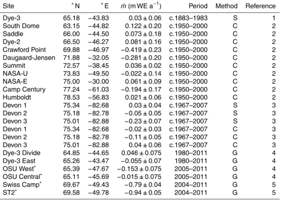
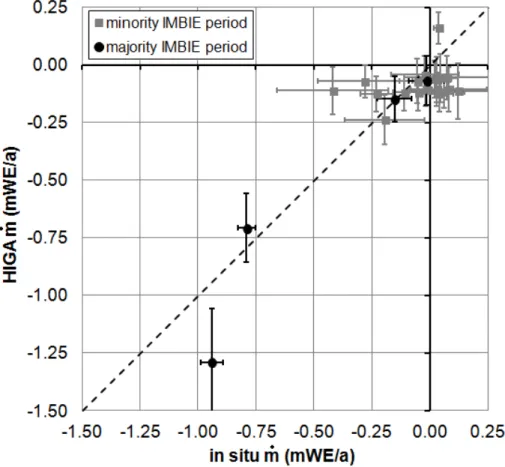
After reviewing the glaciology literature, we find 23 previously published point mea-surements of in situ mass balance across the Canadian Arctic and Greenland (Table 2). We compare these in situ observations to the specific mass balance (i.e.per unit ice

10

area) inferred from our HIGA product, which is calculated as mass balance (i.e. per unit area) divided by fractional ice coverage (Fig. 7; Colgan et al., 2013). Of these 23 sites, there are only four sites at which the majority of the in situ observation period falls within the IMBIE period. At three of these four sites (OSU West, OSU Central and Swiss Camp) the HIGA ˙m is within error of y ₌x (Fig. 8). HIGA ˙m appears to

over-15

estimate observed mass loss at ST2, beyond the uncertainty approximated by local ensemble spread. We note that as spatial heterogeneity in mass balance increases towards the ice sheet margin, a point measurement of ˙mis less likely to be representa-tive of a larger area (e.g. 26 by 26 km) in comparison to the ice sheet interior. Although the ˙m values observed at the remaining 19 sites are not directly comparable to HIGA

20

˙

mvalues due to substantial differences in observation periods, HIGA ˙m is still within error ofy₌xat the majority of these sites. The majority of historical ˙mobservations lie beneathy₌x, which is consistent with the notion that mass balance has generally de-creased since these historical observation periods. For the four sites with a time span consistent with the IMBIE period, the root mean squared difference (RMSD) between

25

TCD

HIGA mass balance product for Greenland and the

Canadian Arctic

W. Colgan et al.

Title Page

Abstract Introduction

Conclusions References

Tables Figures

◭ ◮

◭ ◮

Back Close

Full Screen / Esc

Printer-friendly Version Interactive Discussion

Discussion

P

a

per

|

D

iscussion

P

a

per

|

Discussion

P

a

per

|

Discuss

ion

P

a

per

|

The overarching message of our validation attempt is that there is an urgent need for in situ mass balance measurements in order to calibrate and validate higher reso-lution remotely sensed mass balance products. Presently, the only four sites available for direct comparison during the IMBIE period all lie south of 70◦N on the Greenland Ice Sheet proper. These in situ observations sample neither regions of high mass loss,

5

where dynamic drawdown rates can exceed>2 m WE a−1, nor peripheral ice caps and glaciers, which comprise ∼15 % of Greenland’s mass loss (Bolch et al., 2013; Col-gan et al., 2013). Given the decadal-scale temporal resolution of both coffee can and strain network approaches, it may be possible to collect in situ observations in the near future that have validation utility for the (now historic) IMBIE period. For example,

com-10

bining observed strain rates recovered in 2015 with 15 yr mean surface balance data would essentially produce an ˙m estimate for the 2000 to 2015 period, which closely approximates the anticipated GRACE mission duration. While this would only be pos-sible at sites with appropriate dynamic response timescales, this could greatly improve the inventory of in situ ˙mvalues available for validating both current and future higher

15

resolution satellite gravimetry-derived mass balance products.

4.2 Spatial partition of the continuity equation

The mass balance ( ˙m) at any point on a glacier is the difference between surface mass balance ( ˙b) and the horizontal divergence of ice flux (∇Q), as described by the transient glacier continuity equation:

20

˙

m₌b˙− ∇Q (7)

Differencing HIGA ˙mwith an independent estimate of surface mass balance allows the ice dynamic portion of mass balance to be solved as a residual (Fig. 9). We employ modelled ˙bover the IMBIE period (2004 to 2010) from the regional climate model MAR

25

TCD

HIGA mass balance product for Greenland and the

Canadian Arctic

W. Colgan et al.

Title Page

Abstract Introduction

Conclusions References

Tables Figures

◭ ◮

◭ ◮

Back Close

Full Screen / Esc

Printer-friendly Version Interactive Discussion

Discussion

P

a

per

|

D

iscussion

P

a

per

|

Discussion

P

a

per

|

Discuss

ion

P

a

per

the identification of an accumulation bias in MAR (version 2.1), which resulted in an RMSE of 46 % (24 %) with local ˙b observations above (below) 1500 m elevation (Ver-non et al., 2013), MAR (version 3.2) has been tuned with 86 spatially distributed ice core-derived accumulation records (Box et al., 2013). MAR (version 3.2) reproduces local surface mass balance observations with an RMSE of∼20 %, and ice sheet wide

5

net surface mass balance with an uncertainty of∼10 % (Fettweis et al., 2013). Thus, for the purposes of partitioning the transient continuity equation at 26 km resolution, we take uncertainty in local MAR (version 3.2) ˙b as ±20 %. Solving ∇Q as a resid-ual inherently compounds the uncertainties in both ˙b and ˙m, which we assume sum quadratically. Given the difficulties associated with assessing contemporary∇Qeither

10

from first principles numerical modelling or remotely sensed observations, we suggest that there is value in solving transient∇Qas a residual, despite the relatively high con-sequent uncertainty, which approaches 1 m WE a−1 near the terminus of Jakobshavn Isbrae (Fig. 10).

The residual∇Qfield generally exhibits divergence of horizontal flux throughout the

15

ice sheet interior (e.g.−∇Q) and convergence of horizontal flux (e.g.+∇Q) around the ice sheet periphery (Fig. 9). This is consistent with negative (submerging) vertical ice velocities in the ice sheet accumulation region, and positive (emerging) vertical ice ve-locities in the ice sheet ablation region. Closer inspection, however, reveals contrasting ice dynamic signatures of predominately marine-terminating portions of the ice sheet

20

(e.g. Southeast Greenland and Geikie Plateau) and predominately land-terminating portions of the ice sheet (e.g. North Greenland and Southwest Greenland). In land-terminating regions there is a wide band of convergent (or emergent) ice flux along the ice sheet periphery, while in marine-terminating regions the ice flux is divergent (or submergent) along the ice sheet periphery. We discuss an anomalous small region of

25

convergent ice flux in north central Greenland, where divergent ice flux would normally be expected, in Sect. 4.3.

TCD

HIGA mass balance product for Greenland and the

Canadian Arctic

W. Colgan et al.

Title Page

Abstract Introduction

Conclusions References

Tables Figures

◭ ◮

◭ ◮

Back Close

Full Screen / Esc

Printer-friendly Version Interactive Discussion

Discussion

P

a

per

|

D

iscussion

P

a

per

|

Discussion

P

a

per

|

Discuss

ion

P

a

per

|

sites on the Greenland Ice Sheet (Hamilton and Whillans, 2002), and find that only half are within error ofy ₌x (Fig. 11). Implicit in this comparison is the assumption that any changes in ice velocity at high elevation between the c.1950 to 2000 period and the IMBIE period are negligible (Joughin et al., 2010). Residual∇Q values systemat-ically underestimate in situ vertical velocities at all but one site (NASA-E). Assuming

5

this discrepancy can be explained by a combination of both MAR model or HIGA al-gorithm error, this systematic bias towards less horizontal divergence of ice flux than historically observed may stem from either HIGA-inferred ˙m systematically overesti-mating true ˙m, or MAR-derived ˙b systematically underestimating true ˙b (Fig. 8). By virtue of solving∇Q as a residual, any overestimation (underestimation) of ˙m ( ˙b)

re-10

sults in a direct underestimation of ∇Q (Eq. 7). Given a historical MAR bias towards overestimating accumulation in the ice sheet interior (Vernon et al., 2013), we spec-ulate that our apparent underestimation of residual ∇Q more likely stems from over-estimated HIGA-inferred ˙m than underestimated MAR-modeled ˙b. We note, however, that aggregated across the high elevation ice sheet interior, which we take as the area

15

enclosed by the 2000 m elevation contour, HIGA-inferred ˙m suggests a mass balance of 10±4 Gt a−1during the IMBIE period. This slightly positive high elevation mass bal-ance, equivalent to∼1 cm WE a−1ice thickening, is consistent with in situ observations that the high elevation region is close to zero balance (Thomas et al., 2001).

4.3 Millennial scale ice dynamics

20

The Greenland Ice Sheet is assumed to have been in near equilibrium during the 1961 to 1990 reference period (van den Broeke et al., 2009). The residual ∇Q field we present here, however, suggests that ice dynamics may be contributing to a sub-stantial mass gain in the ice sheet interior (Fig. 9). This is especially evident in a region of convergent ice flux in north central Greenland, where divergent ice flux would

nor-25

HIGA-TCD

HIGA mass balance product for Greenland and the

Canadian Arctic

W. Colgan et al.

Title Page

Abstract Introduction

Conclusions References

Tables Figures

◭ ◮

◭ ◮

Back Close

Full Screen / Esc

Printer-friendly Version Interactive Discussion

Discussion

P

a

per

|

D

iscussion

P

a

per

|

Discussion

P

a

per

|

Discuss

ion

P

a

per

inferred ˙m, we note that this apparent artifact is consistent with the magnitude and spatial distribution of subtle mass gain anticipated from millennial scale ice dynamics. Transient mass gain associated with ice dynamics is expected to be most evident near flow divides in north central Greenland due to: (i) nearly vertical ice flow, which makes changes in ice surface elevation due to ice dynamics more pronounced than areas

5

where ice flow approaches surface-parallel, and (ii) relatively low accumulation rates, which amplifies a given anomaly in ice dynamics in comparison to higher accumulation sites.

The Greenland Ice Sheet is estimated to have been ∼15 % thinner than present during the peak of the Wisconsin glaciation∼21 kaBP, due to the smaller crystal size

10

and increased solute concentration of Wisconsin ice in comparison to Holocene ice (Reeh, 1985). Consequently, the ice sheet is hypothesized to be presently undergoing a subtle high elevation thickening due to the gradual replacement of softer Wiscon-sin ice with firmer (or more viscous) Holocene ice. Potentially analogous long term dynamic ice cap thickening has been observed in the Canadian Arctic (Colgan et al.,

15

2008). In Greenland, this subtle high elevation thickening has a hypothesized rate of

∼1 cm WE a−1 (Reeh, 1985), which is corroborated by coarse resolution (20 km) 3-D thermo-mechanical ice flow modelling (Huybrechts, 1994). Reeh and Gundestrup (1985) explicitly attribute an in situ mass balance of 3±6 cm WE a−1observed at Dye-3 to millennial-scale ice dynamics associated with the Wisconsin-Holocene transition. At

20

seven additional widely distributed high elevation sites (South Dome, Saddle, Dye-2, Summit, NASA-E, Camp Century and Humboldt), which are unlikely to be influenced by enhanced flow mechanisms (i.e. surface velocity<27 m a−1), in situ co_ffee can mea-surements similarly identify a mean thickening of 3±12 cm WE a−1, including an obser-vation of net thinning at Camp Century (Hamilton and Whillans, 2002).

25

TCD

HIGA mass balance product for Greenland and the

Canadian Arctic

W. Colgan et al.

Title Page

Abstract Introduction

Conclusions References

Tables Figures

◭ ◮

◭ ◮

Back Close

Full Screen / Esc

Printer-friendly Version Interactive Discussion

Discussion

P

a

per

|

D

iscussion

P

a

per

|

Discussion

P

a

per

|

Discuss

ion

P

a

per

|

(e.g.+ve∇Q), and thus improves notional consistency with radial flow extending down-wards from the local flow divides (Fig. 12). Application of a secular thickening trend also acts in favour of reducing the discrepancy between residual∇Qand in situ vertical ice velocities at sites above the PARCA perimeter (Fig. 11). This secular mass gain trend is within the range of theoretical, modelled and observed thickening trends attributed to

5

the ongoing Wisconsin-Holocene transition (Reeh, 1985; Reeh and Gundestrup, 1985; Huybrechts, 1994; Hamilton and Whillans, 2002). In order to explicitly acknowledge the role of millennial scale ice dynamics when spatially partitioning the transient glacier continuity equation, shorter term (ST) and longer term (LT) ice dynamics may be con-ceptualized as:

10

˙

m₌b˙− ∇Q_ST− ∇Q_LT (8)

where centurial to millennial scale dynamic mass changes occurring during reference period are attributed to longer term ice dynamics (∇Q_LT), and annual to decadal scale dynamic mass changes occurring since reference period are attributed to shorter term

15

ice dynamics (∇Q_ST; Fig. 12).

While acknowledging the role of subtle millennial scale high elevation thickening may be important in achieving a spatial partition of ˙b and ∇Q that is theoretically consistent with the transient glacier continuity equation, it challenges the assumption that the Greenland Ice Sheet was in near-equilibrium during the recent 1961 to 1990

20

reference climatology period (cf. van den Broeke et al., 2009). A thickening rate of 2 cm WE a−1distributed uniformly across the 9.8×105km2of ice sheet area above the nominal 2000 m elevation PARCA perimeter is equivalent to an annual mass gain of

∼18 Gt. While this signal is within error of estimates of ice sheet scale annual accumu-lation or iceberg calving, it is non-trivial (∼8 %) and opposite in sign in comparison

25

transi-TCD

HIGA mass balance product for Greenland and the

Canadian Arctic

W. Colgan et al.

Title Page

Abstract Introduction

Conclusions References

Tables Figures

◭ ◮

◭ ◮

Back Close

Full Screen / Esc

Printer-friendly Version Interactive Discussion

Discussion

P

a

per

|

D

iscussion

P

a

per

|

Discussion

P

a

per

|

Discuss

ion

P

a

per

tion. Invoking Occam’s razor (e.g. Anderson, 2002), an overestimation of HIGA ˙m is the most likely explanation for our systematic underestimation of residual∇Q values; the consistency of our apparent ∇Q artifact with the magnitude and spatial distribu-tion of subtle mass gain anticipated from millennial scale ice dynamics is curious, but likely entirely coincidental. A thorough understanding of high elevation mass balance

5

during the 1961 to 1990 reference climatology period, however, to verify∇Q_LT≈0, is required before excluding millennial scale ice dynamics as a factor in contemporary high elevation mass balance.

5 Summary remarks

The mass balance product that we derive through iterative inversion is simultaneously

10

consistent with glacier inventory, cryosphere-attributed mass changes derived from satellite gravimetry, and ice surface elevation changes derived from airborne and satel-lite altimetry. This HIGA product combines the complementary strengths of gravimetry and altimetry to refine direct measurements of cryosphere-attributed mass change to relatively high spatial resolution. While we have attempted to validate HIGA mass

bal-15

ance values against in situ observations, we find only a handful of locations throughout Greenland and the Canadian Arctic where mass balance was measured over a time period directly comparable to the IMBIE period (2004 to 2010). We therefore identify an urgent need for additional in situ measurements of mass balance to calibrate higher resolution remotely sensed mass balance products.

20

Of the 316±37 Gt a−1 of mass loss over the Canadian Arctic and Greenland dur-ing the IMBIE period, we attribute 217±20 Gt a−1 to the ice sheet proper, and 38±6 Gt a−1 and 50±8 Gt a−1 to peripheral glaciers in Greenland and the Canadian Arctic, respectively. We note that these mass loss estimates are dependent on the spheri-cal harmonic representation with which we initialized our iterative inversion. Employing

25

TCD

HIGA mass balance product for Greenland and the

Canadian Arctic

W. Colgan et al.

Title Page

Abstract Introduction

Conclusions References

Tables Figures

◭ ◮

◭ ◮

Back Close

Full Screen / Esc

Printer-friendly Version Interactive Discussion

Discussion

P

a

per

|

D

iscussion

P

a

per

|

Discussion

P

a

per

|

Discuss

ion

P

a

per

|

previously published estimates, while the mass loss we assess to the Canadian Arctic is within overlapping uncertainties of previously published estimates. Given that Green-land’s peripheral glaciers, which comprise<5 % of Greenland’s ice covered area, ap-pear to be contributing ∼15 % of the aggregate Greenland mass loss observed by satellite gravimetry, GRACE-derived estimates of “Greenland” mass loss cannot

rea-5

sonably be taken as synonymous with “Greenland ice sheet” mass loss. Comparisons of GRACE-derived mass loss should therefore be limited to other mass balance tech-niques (i.e. input-output or altimetry) that sample both the ice sheet and its peripheral glaciers.

Combining HIGA mass balance with surface mass balance from the regional climate

10

model MAR has allowed us to solve the transient glacier continuity equation at 26 km resolution across Greenland during the December 2003 to December 2010 period. The residual horizontal divergence of flux field (∇Q) is generally consistent with the notion of divergent ice flow (submergent velocities) in the ice sheet accumulation region and convergent ice flow (emergent velocities) in land-terminating ablation regions. Marginal

15

areas with divergent ice flow generally correspond to regions of marine-terminating glaciers, consistent with a dynamic mass loss mechanism. This first-order partition of the transient continuity equation, however, infers a small pocket of convergent ice flow in North Central Greenland, which is not consistent with theoretical and observed radial flow ice velocities. We speculate that a systematic underestimation of observed vertical

20

ice velocities stems from an overestimation of HIGA-inferred mass balance in the ice sheet interior. We note, however, that this apparent artifact in the flux divergence field is consistent in magnitude and spatial distribution with subtle high elevation mass gain, which has been previously postulated in association with the downward advection of the Wisconsin-Holocene transition within the ice sheet.

25

Supplementary material related to this article is available online at

TCD

HIGA mass balance product for Greenland and the

Canadian Arctic

W. Colgan et al.

Title Page

Abstract Introduction

Conclusions References

Tables Figures

◭ ◮

◭ ◮

Back Close

Full Screen / Esc

Printer-friendly Version Interactive Discussion

Discussion

P

a

per

|

D

iscussion

P

a

per

|

Discussion

P

a

per

|

Discuss

ion

P

a

per

Acknowledgements. This work was funded by NASA award NNX10AR76G and DFF award FNU 11-115166. This work utilized the Janus supercomputer, which is supported by NSF award CNS-0821794 and the University of Colorado Boulder. The Janus supercomputer is a joint ef-fort of the University of Colorado Boulder, the University of Colorado Denver and the National Center for Atmospheric Research. W. C. thanks Joel Frahm for his continued assistance

work-5

ing with Janus. M. C. was supported by PROMICE and GlacioBasis with funds from the Danish Energy Agency. We thank Ken Jezek very much for sharing his field data and reviewing our interpretation of the mass balance of the Ohio State University clusters in South Greenland.

References

Alley, R., Spencer, M., and Anandakrishnan, S.: Ice-sheet mass balance: assessment,

attribu-10

tion, and prognosis, Ann. Glaciol., 46, 1–7, 2007.

Anderson, D.: Occam’s Razor: simplicity, complexity„ and global geodynamics, P. Am. Philos. Soc., 146, 56–70, 2002.

Arendt, A., Bolch, T., Cogley, J., Gardner, A., Hagen, J., Hock, R., Kaser, G., Pfeffer, W., Mo-holdt, G., Paul, F., Radic, V., Andreassen, L., Bajracharya, S., Beedle, M., Berthier, E.,

Bham-15

bri, R., Bliss, A., Brown, I., Burgess, E., Burgess, D., Cawkwell, F., Chinn, T., Copland, L., Davies, B., De Angelis, H., Dolgova, E., Filbert, K., Forester, R., Fountain, A., Frey, H., Gif-fen, B., Glasser, N., Gurney, S., Hagg, W., Hall, D., Haritashya, U., Hartmann, G., Helm, C., Herreid, S., Howat, I., Kapustin, G., Khromova, T., Kienholz, C., Koenig, M., Kohler, J., Kriegel, D., Kutuzov, S., Lavrentiev, I., LeBris, R., Lund, J., Manley, W., Mayer, C., Miles, E.,

20

Li, X., Menounos, B., Mercer, A., Moelg, N., Mool, P., Nosenko, G., Negrete, A., Nuth, C., Pettersson, R., and Racoviteanu, A.: Randolph Glacier Inventory version 2.0: A Dataset of Global Glacier Outlines, Global Land Ice Measurements from Space, Digital Media, Boulder Colorado, USA, 2012.

Bohlen, T. and Saenger, E.: Accuracy of heterogeneous staggered-grid finite-difference

model-25

ing of Rayleigh waves, Geophysics, 71, T109–T115, 2006.