www.the-cryosphere.net/2/117/2008/
© Author(s) 2008. This work is distributed under the Creative Commons Attribution 3.0 License.
The Cryosphere
Estimation of the Greenland ice sheet surface mass balance for the
20th and 21st centuries
X. Fettweis1, E. Hanna2, H. Gall´ee3, P. Huybrechts4, and M. Erpicum1
1D´epartement de G´eographie, Universit´e de Li`ege, Li`ege, Belgium 2Department of Geography, University of Sheffield, Sheffield, UK
3LGGE – Laboratoire de Glaciologie et G´eophysique de l’Environnement, Grenoble, France 4Departement Geografie, Vrije Universiteit Brussel, Brussel, Belgium
Received: 6 March 2008 – Published in The Cryosphere Discuss.: 9 April 2008
Revised: 19 August 2008 – Accepted: 4 September 2008 – Published: 24 September 2008
Abstract.Results from a regional climate simulation (1970– 2006) over the Greenland ice sheet (GrIS) reveals that more than 97% of the interannual variability of the modelled Sur-face Mass Balance (SMB) can be explained by the GrIS summer temperature anomaly and the GrIS annual precip-itation anomaly. This multiple regression is then used to empirically estimate the GrIS SMB since 1900 from clima-tological time series. The projected SMB changes in the 21st century are investigated with the set of simulations per-formed with atmosphere-ocean general circulation models (AOGCMs) of the Fourth Assessment Report of the Inter-governmental Panel on Climate Change (IPCC AR4). These estimates show that the high surface mass loss rates of re-cent years are not unprecedented in the GrIS history of the last hundred years. The minimum SMB rate seems to have occurred earlier in the 1930s and corresponds to a zero SMB rate. The AOGCMs project that the SMB rate of the 1930s would be common at the end of 2100. The temperature would be higher than in the 1930s but the increase of accu-mulation in the 21st century would partly offset the acceler-ation of surface melt due to the temperature increase. How-ever, these assumptions are based on an empirical multiple regression only validated for recent/current climatic condi-tions, and the accuracy and time homogeneity of the data sets and AOGCM results used in these estimations constitute a large uncertainty.
1 Introduction
Mass balance variations of the GrIS play an important role in global sea level fluctuations and oceanic THC changes.
Correspondence to:X. Fettweis ([email protected])
On the one hand, GrIS mass balance changes appear to have contributed several metres to some of the sea-level fluctua-tions since the last interglacial period known as the Eemian, 125 K yr BP (Cuffey and Marshall, 2000) and are expected to contribute to sea-level rise under the projected future global warming throughout this century (Meehl et al., 2007). On the other hand, increases in the freshwater flux from the Green-land ice sheet (run-off of the surface melt water, basal melt-ing and glacier discharge) could perturb the THC by reduc-ing the density contrast drivreduc-ing the thermohaline circulation (Rahmstorf et al., 2005). Any weakening of the THC in response to a surface warming and an increasing freshwa-ter flux induced by global warming (Gregory et al., 2005; Swingedouw et al., 2006) would reduce the heat input to the North Atlantic ocean and subsequently reduce the warming in regions including Europe. The IPCC 4th Assessment Re-port (IPCC AR4) projected that the Greenland ice sheet is likely to lose mass because the increasing run-off is expected to exceed the precipitation increase in a warmer climate but did not expand on the individual model estimates or mass balance components (Meehl et al., 2007).
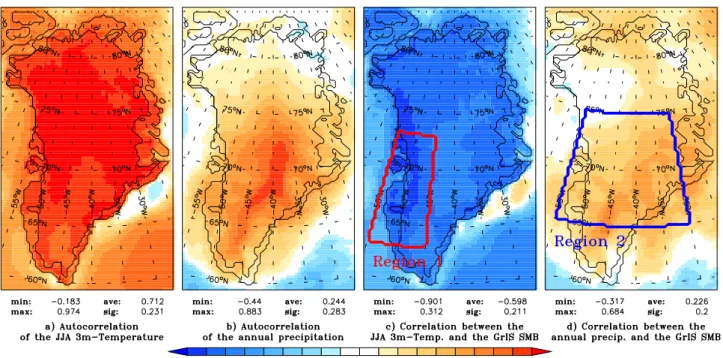
Fig. 1. Left: spatial autocorrelation of the(a)JJA 3 m-temperature and(b)annual precipitation simulated by MAR over the period 1970– 1999. The spatial autocorrelation is defined as the correlation between time series of the average ice-sheet summer temperature and annual total ice-sheet precipitation with the respective temperature/precipitation values for each grid point. Right: the correlation between the time series of the MAR-simulated GrIS SMB and(c)JJA 3 m-temperature and(d)annual precipitation at each grid location. Minimum and maximum values are indicated as well as the ice sheet average and the standard deviation. Finally, this figure shows the regions quoted in the text. Region 1: 55◦W≤longitude≤45◦W and 63◦N≤latitude≤73◦N. Region 2: 55◦W≤longitude≤30◦W and 65◦N≤latitude≤75◦N.
near past and future GrIS SMB rates are presented in Sect. 3 and Sect. 4, respectively. Section 5 contains a discussion of the results.
2 Method
To a first approximation, the GrIS SMB variability (1SMBGrIS) is driven by the GrIS annual precipitation
anomaly (1Pyr) minus the GrIS meltwater run-off rate
vari-ability. According to Box et al. (2004) and Fettweis (2007), the run-off rate variability can be approximated by the GrIS summer (from 1 June to 31 August) 3 m-temperature (1Tjja)
to give this multiple regression:
1SMBGrIS≃a1Tjja+b1Pyr (1)
whereaandbare constant parameters. These parameters are determined by solving the multiple regression equation using the simulated GrIS SMB anomaly time series and both JJA temperature and annual precipitation anomaly time series.
By using de-trended results simulated by MAR, a correla-tion coefficient of 0.97 is obtained between the simulated and estimated GrIS SMB anomaly from Eq. (1) over the period 1970–1999. The root mean square error (RMSE) represents 25% of the GrIS SMB anomaly standard deviation. Such a correlation motivated us to use this equation to extend the es-timate of the SMB variability with the help of climatological
time series and the outputs from analyses and the AOGCMs used in the IPCC AR4. The 30-yr reference period (1970– 1999) is chosen because it covers most of the available data sets and model results used in this study.
Table 1.Five climatological data sets used in this paper to estimate the GrIS SMB.
Abbreviation Name Period Resolution Web site Reference
CRU Climate Research Unit TS 2.1 1901–2002 0.5◦ http://www.cru.uea.ac.uk Mitchell and Jones (2005) ECMWF ECMWF (Re)-Analysis 1958–2006 1.125◦ http://www.ecmwf.int Uppala et al. (2005) GHCN Global Histo. Climato. Network 2 1900–2006 5◦ http://lwf.ncdc.noaa.gov/ Peterson and Vose (1997) NCEP NCEP/NCAR Reanalysis 1 1948–2006 ∼2◦ http://www.cdc.noaa.gov/cdc/data.ncep.reanalysis.html Kalnay et al. (1996) UDEL Arctic Land-Surface TS 1.01 1930–2000 0.5◦ http://climate.geog.udel.edu/∼climate/html pages/download.html#ac temp ts2
Table 2.Correlation coefficient between the de-trended annual temperature (resp. precipitation) anomaly averaged over Region 1 (resp. Re-gion 2) from the different data sets and simulated by the MAR model over the reference period (1970–1999). The correlation coefficient as well as the RMSE (in km3) between the de-trended GrIS SMB modelled by MAR and the SMB estimated by temperature/precipitation de-trended anomaly time series are also shown. Finally, the parametersaandb(computed by using de-trended normalized time series) are listed as well as their ratio and the standard error of these paramaters.
Name 1T corr. 1Pcorr. 1SMB corr. RMSE a b k=a/b
CRU 0.79 0.84 0.81 64.6 −66.6±13 49.4±13 −1.35(−2.16,−0.87)
ECMWF 0.92 0.94 0.89 49.2 −65.1±10 62.6±10 −1.04(−1.42,−0.77) GHCN 0.83 0.82 0.83 61.4 −61.8±12 53.2±12 −1.16(−1.82,−0.75) NCEP 0.91 0.90 0.89 49.6 −75.1±10 61.4±10 −1.22(−1.62,−0.92) UDEL 0.86 0.80 0.83 61.0 −73.7±12 47.7±12 −1.65(−2.61,−1.09)
MAR 1.0 1.0 0.97 28.5 −63.3±6 64.8±6 −0.98(−1.18,−0.81)
Fig. 3.The GrIS SMB anomaly simulated by the MAR model and estimated with Eq. (1) by using temperature/precipitation anoma-lies simulated by MAR, derived using a positive degree-day and run-off/retention model based on ECMWF reanalysis Hanna et al. (2008) and estimated by using temperature/precipitation anomaly from the ECMWF (re)analysis, and simulated by the Polar MM5 model Box et al. (2006). The reference period is 1970–1999 and the temperature and precipitation anomaly are taken from Region 1 and 2 described in Fig. 1.
data sets used hereafter (see Table 2), while the choice of the boundaries of these regions does not significantly impact the results. Both regions chosen are therefore the same for all data sets.
A good agreement between the modelling from MAR and from Hanna et al. (2008) (called Hanna08 hereafter) and the estimates of the GrIS SMB anomaly by using temperature (respectively precipitation) anomaly on Region 1 (resp. 2) can be seen in Fig. 3. This figure also compares the GrIS SMB simulated by the Polar MM5 model (Box et al., 2006). The differences between these three models are briefly de-scribed in Fettweis (2007). The interannual variability com-pares well between the models before 2000 while this last one is higher in the MAR model than in the Hanna08 time se-ries. The Hanna08 run-off model is forced by monthly mean atmospheric fields from the ECMWF (re)analysis which
could underestimate the impact of extreme warm events dur-ing the summer and then reduce the interannual variability. After 2001, large discrepancies however occur between the models. First, in the 2000s, there is a succession of nega-tive SMB anomalies inducing an acceleration of the melt the following year due to the albedo feedback and the humid-ification of the snowpack. These feedbacks could be over-estimated in the MAR model compared with other models. In addition, these feedbacks are not taken into account in the (Polar) MM5 model because the surface model is reini-tialized every day in MM5. Secondly, different sensitivities of the various SMB models to several profound changes in the ECMWF model configuration/resolution used to produce ECMWF operational analyses after 2002 (as opposed to the fixed model scheme of ERA-40 (Uppala et al., 2005) for the period 1958–2001) could explain the differences in the mod-els since 2002. The disagreement in the 2000s explains why we did not extend the 30-yr reference period (1970–1999) to the 2000s.
Finally, Oerlemans et al. (2005) use a similar estimation of Eq. (1) which is in total agreement with that we have found in Eq. (1) by using the MAR simulated time series. Using the same units as Oerlemans et al. (2005), we obtain a coef-ficienta of−43.3 mm/K compared with−49 in Oerlemans et al. (2005) and a coefficientb of 3 mm/% compared with 3.8 in Oerlemans et al. (2005). If we use the SMB time series from Hanna08 and the temperature and precipitation anomalies time series in Region 1 and 2 from the ERA-40 reanalysis in Eq. (1) a coefficienta(resp.b) of−49.4 mm/K (resp. 3.4 mm/%) is found, which fully agrees with those found by Oerlemans et al. (2005). These values are also in agreement with Box et al. (2006).
3 Surface mass balance in the 20th century
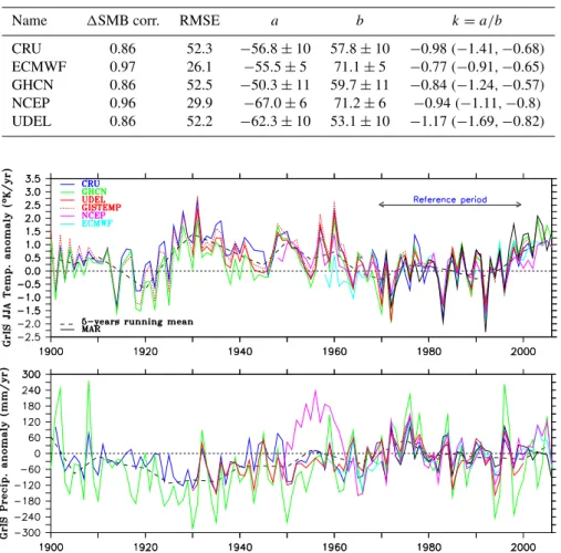
Table 3.The same as Table 2 but by using results simulated by Hanna08 in the left part of Eq. (1).
Name 1SMB corr. RMSE a b k=a/b
CRU 0.86 52.3 −56.8±10 57.8±10 −0.98(−1.41,−0.68) ECMWF 0.97 26.1 −55.5±5 71.1±5 −0.77(−0.91,−0.65) GHCN 0.86 52.5 −50.3±11 59.7±11 −0.84(−1.24,−0.57) NCEP 0.96 29.9 −67.0±6 71.2±6 −0.94(−1.11,−0.8) UDEL 0.86 52.2 −62.3±10 53.1±10 −1.17(−1.69,−0.82)
Fig. 4.Time series of the GrIS temperature (resp. precipitation) anomaly computed for Region 1 (resp. 2) from the different data sets listed in Table 1. In red dashed, the time series from GISTEMP (available at http://data.giss.nasa.gov/). Anomalies are with respect to 1970–1999. The 5-yr running mean of the averaged anomalies of the available data sets is shown in dashed black.
temperature/precipitation anomaly time series from the data set averaged on Region 1/Region 2 in the right part. The high correlation coefficient(>0.8) between the GrIS SMB anomaly simulated by MAR (resp. Hanna08) and the one es-timated by the data sets following Eq. (1) over 1970–1999 (see Tables 2 and 3) motivated us to extend empirically the SMB anomaly estimation to the whole period covered by the data sets by using the same previously determined param-etersa andb. These parameters are computed over 1970– 1999 by using de-trended (i.e. with a zero trend) time series to minimise the dependence on the reference period and are applied after that to the whole time series (without correction of the trend). The anomalies refer then to the period 1970– 1999. In addition, the use of de-trended time series of anoma-lies to compute the parametersaandbrather than time series of values provides a better homogeneity between the differ-ent data sets and the MAR (resp. Hanna08) model. Before continuing, it should be noted that these data set-based SMB anomaly estimates should be considered with caution.
– Firstly, these estimates are based on Eq. (1) which does not fully explain the SMB variability and uses results from the MAR and Hanna08 models (not direct obser-vations) for the calibration.
– Secondly, by using constant parametersaandbthrough the whole period covered by the climatic dataset, we assume that the dependence of the SMB on the tem-perature/precipitation anomaly are the same as during 1970–1999. That is why we chose to use de-trended time series to minimise this impact.
– In addition, we assume that the data set is homogeneous through the whole period, which is not guaranteed as, for example, in the ECMWF time series after 2002. – We assume also that the variability in Region 1 and 2
Fig. 5. (a)Time series of the estimated GrIS SMB anomaly using the SMB variability simulated by MAR (to determine the parametersa andbin Eq. (1)) and anomalies from the different data sets listed in Table 1 since 1900 until 2006. The reference period is 1970–1999 over which the GrIS SMB simulated by MAR and by Hanna08 is around 350 km3yr−1. The 5-yr running mean of the ensemble mean is shown in dashed black.(b)The same as (a) but using the Hanna08 results to determine the parametersaandbin Eq. (1).
and decadal variability (for the future projections). In addition, we assume by using a linear equation that a doubling in, for instance, the temperature deviation will result in a doubling of the melt anomaly.
– Finally, there are not many in-situ observations (on which the data sets are based) available over Greenland. Such data are collected along the coast by the Danish Meteorological Institute (DMI) weather stations. They are consequently not representative for the GrIS (Fet-tweis et al., 2005; Cappelen et al., 2001), although Hanna et al. (2008) show good correspondence between DMI and Swiss Camp (west flank of GrIS) summer tem-perature variations since 1990. Nevertheless, we can as-sume that the interannual variability is less sensitive to the lack of measurements over the GrIS, the more so since the variability along the coast is a good proxy for the whole GrIS variability according to Figs. 1 and 2. Figure 4 plots the time series of anomalies for the dif-ferent datasets from 1900 to 2006. As these datasets are mainly based on the same in situ observations, the temper-ature time series compare very well. All the series unani-mously show warm periods around 1930, 1950 and 1960 in full agreement with previous studies based on coastal DMI weather station observations (Box, 2002; Box and Cohen, 2006; Vinther et al., 2006). The rate of warming in 1920– 1930 is the most spectacular as pointed out by Chylek et al. (2006). Finally, Greenland climate was colder around 1920 and, in the 1970s and 1980s. The temperature
mini-mum (resp. maximini-mum) seems to have occurred in 1992 af-ter the Mont Pinatubo eruption (resp. in 1931). The warm summers of recent years (1998, 2003, 2005), associated with large melt extent areas (Fettweis et al., 2007), seem to be less warm than these of the 1930s, as also pointed out by Hanna et al. (2007).
Concerning the precipitation time series, the agreement among them is less obvious and large disparities occur as for example with the NCEP precipitation time series in the 1950s. In addition, the interannual variability is more sig-nificant in the GHCN precipitation time series because only one or two pixels with data are available in Region 2 (Three pixels with temperature data are available in Region 1). This suggests that the precipitation variability in the GHCN time series is rather the variability measured by one or two coastal DMI weather stations. However, the series show all a small negative anomaly in the 1930s and positive in 1970s but these anomalies are less significant than the temperature anoma-lies. Finally, the correlation of the de-trended time series of the data sets with the MAR anomalies is better for tempera-ture than for precipitation (see Table 2). The precipitation is more difficult to simulate and to measure (especially snow-fall) which might explain these discrepancies.
Table 4. Twenty-three AOGCMs from the IPCC AR4 (Randall et al., 2007) used in this paper. This data comes from the World Climate Research Programme’s (WCRP’s) Coupled Model Intercomparison Project phase 3 (CMIP3) multi-model dataset available at http://www-pcmdi.llnl.gov/.
Model ID Sponsors, Country
BCCR-BCM2.0 Bjerknes Centre for Climate Research, Norway CCSM3 National Center for Atmospheric Research, USA
CGCM3.1(T47 & T63) Canadian Centre for Climate Modelling and Analysis, Canada CNRM-CM3 M´et´eo-France/Centre National de Recherches M´et´eorologiques, France CSIRO-MK3.0 & 3.5 Commonwealth Scientific and Industrial Research
Organisation Atmospheric Research, Australia ECHAM5-MPI-OM Max Planck Institute for Meteorology, Germany
ECHO-G Meteorological Institute of the University of Bonn, Germany
Meteorological Research Institute of the Korea Meteorological Administration Korea FGOALS-G1.0 National Key Laboratory of Numerical Modeling for Atmospheric Sciences
and Geophysical Fluid Dynamics /Institute of Atmospheric Physics, China GFDL-CM2.0 & 2.1 US Department of Commerce/National Oceanic and Atmospheric
Administration/Geophysical Fluid Dynamics Laboratory, USA
GISS-AOM National Aeronautics and Space Administration /Goddard Institute for Space Studies, USA GISS-EH & ER National Aeronautics and Space Administration /Goddard Institute for Space Studies, USA INM-CM3.0 Institute for Numerical Mathematics, Russia
IPSL-CM4 Institut Pierre Simon Laplace, France
MIROC3.2(hires) & (medres) Center for Climate System Research, National Institute for Environmental Studies, and Frontier Research Center for Global Change, Japan MRI-CGCM2.3.2 Meteorological Research Institute, Japan
PCM National Center for Atmospheric Research, USA
UKMO-HadCM3 & HadGEM1 Hadley Centre for Climate Prediction and Research/Met Office, UK
glacier discharge and the basal melting rate (Reeh et al., 1999; Fettweis, 2007). Tables 2 and 3 list the ratioa/b, i.e. the weight of the temperature variability against the precip-itation variability in the SMB variability. This ratio is ob-tained by using normalized (i.e. with a standard deviation of 1) de-trended temperature/precipitation anomaly time series. On average, this ratio is near−1.0 (−1.5,−0.75). The details of the uncertainty of the ratioa/bis explained in the legend of Table 2. Therefore, the thermal factors influence the SMB sensitivity as much as precipitation changes.
The set of SMB estimates in Fig. 5 agree to give pos-itive anomalies around 1920 and in the 1970s and 1980s. The maximum, confirmed by all data sets, takes place at the beginning of the 1970s with a SMB anomaly near
+200 km3yr−1due to a combination of cold summers and wet years. Over the period 1930–1960 and since the end of 1990s, the estimated SMB is below the 1970–1999 average. The absolute minimum occurred around 1930 with a SMB anomaly near−300 km3yr−1. Secondary (minor) SMB min-ima appear to have occurred in 1950 and 1960, equalling the surface mass loss rates of the last few years (1998, 2003, 2006), although these minima are not confirmed in all data sets. However (Chylek et al., 2007) found also a maximum melt area at the beginning of the 1930s followed by minor maxima in 1950 and 1960. The minimum SMB rates around 1930 are due to exceptionally warm summers combined with dry years inducing SMB rates lower than those currently ob-served, although the effect of human-induced global warm-ing was not perceptible at that time. Around 1950 and 1960, the low SMB rates are mainly explained by positive
temper-ature anomalies. After the 1990s, the GrIS SMB decreases slowly to reach the negative anomalies of the last few years, although the summers of the 2000s were not exceptional compared to 70 yr ago (Chylek et al., 2006).
Finally, the interannual SMB variability was higher in 1960–1990 than in the 1930s and 2000s. During 1960–1990, negative SMB anomalies were mainly succeeded by positive anomalies. By contrast, in the 1930s and 2000s, there is a succession of negative SMB anomalies inducing an acceler-ation of the melt due to the albedo feedback. A high melt-rate year decreases the snow pack albedo for the next year if the winter accumulation is not enough to compensate the melt during the next summer (Fettweis, 2007).
4 Change in the future
In the following section, we assume that the hypotheses made before are still valid in the near future. In that case, AOGCM simulations (Randall et al., 2007) performed for the 4th as-sessment report of the IPCC can be used to project the GrIS SMB anomalies for the 21st century. The projected temper-ature/precipitation anomalies (plotted in Fig. 6) are based on model outputs from the “Climate of the Twentieth Century Experiment” (20C3M) and from the scenario SRES (Special Report on Emission Scenarios) A1B described in Nakicen-ovic et al. (2000). The A1B scenario corresponds to a con-tinuous increase of the atmospheric CO2concentration
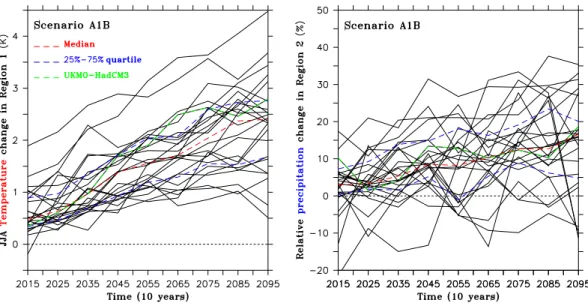
Fig. 6.Time series of temperature (resp. precipitation) anomalies projected by AOGCMs listed in Table 4. The anomalies are decadal means, computed on Region 1 and 2 described previously and refer to the period 1970–1999. The anomalies are based on model outputs from the “Climate of the Twentieth Century Experiment” (20C3M) and from the scenario SRES A1B. Finally, the median (50%), the 25% and 75% quartile values among the 24 models and the UKMO-HadCM3 time series are plotted in red, blue and green, respectively.
scenario was chosen because it is a mid-range scenario and all the IPCC AR4 AOGCMs have outputs for this scenario.
We deduce the projected SMB changes in the future from the IPCC AR4 experiments (Randall et al., 2007) via the fol-lowing algorithm:
1. The time series of the JJA temperature (Ti) taken in Re-gion 1 and the annual precipitation (Pi) taken in Re-gion 2 from the 20C3M experiment are de-trended, cen-tred i.e.
T = 1
30
1999
X
i=1970
Ti =P =0 (2)
and normalized (i.e. with a standard deviation of 1): v
u u t1
29
1999
X
i=1970
Ti2= v u u t1
29
1999
X
i=1970
Pi2=1 (3)
over 1970–1999. The normalisation of theTi andPi time series enables to homogenise the AOGCMs results over 1970–1999.
2. The MAR and Hanna08 results show a standard devia-tion of the GrIS SMB time series around 100 km3yr−1 over the period 1970–1999. Therefore, ifk=a/b, the standard deviation of the SMB estimated by the tem-perature and precipitation time series from the 20C3M experiment is fixed to be 100 km3yr−1, i.e.
v u u t 1 29
1999
X
i=1970
(aTi+bPi)2
=a v u u t 1 29
1999
X
i=1970
(Ti+ 1 kPi)
2fork= a
b
=100 km3yr−1 (4)
which enables the computation ofaandbif the param-eterkis known. Previous results listed in Tables 2 and 3 show a parameterkaround−1.0 (−1.5,−0.75). Here, we will computeaandbforkfixed at−1.
3. For each decade between the 2010s and the 2090s, the mean projected summer temperature (resp. annual pre-cipitation) in Region 1 (resp. Region 2) is retrieved from the SRESA1B scenario. Afterwards, the mean 1970– 1999 temperature (resp. precipitation) from the 20C3M experiment is subtracted from the projected temperature (resp. precipitation) to compute anomalies which we di-vide by the normalisation factor used in Eq. (3) to give this equation:
1SMB=aTSRESA1B−T20C3M st dev(T20C3M)
+bPSRESA1B−P20C3M st dev(P20C3M)
(5)
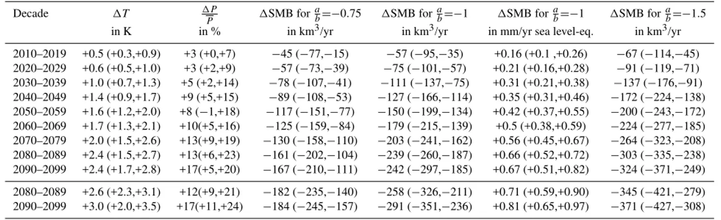
Table 5.Future projections for the 21st century from the ensemble mean of the AOGCMs simulations performed for the IPCC AR4. The two last lines use simulations made for the SRESA2 experiments against SRESA1B for the other ones. The table shows the median (50%), and 25% and 75% quartile values among the 24 models.
Decade 1T 1P
P 1SMB for a
b=−0.75 1SMB for a
b=−1 1SMB for a
b=−1 1SMB for a b=−1.5
in K in % in km3/yr in km3/yr in mm/yr sea level-eq. in km3/yr 2010–2019 +0.5 (+0.3,+0.9) +3 (+0,+7) −45 (−77,−15) −57 (−95,−35) +0.16 (+0.1 ,+0.26) −67 (−114,−45) 2020–2029 +0.6 (+0.5,+1.0) +3 (+2,+9) −57 (−73,−39) −75 (−101,−57) +0.21 (+0.16,+0.28) −91 (−119,−71) 2030–2039 +1.0 (+0.7,+1.3) +5 (+2,+14) −78 (−107,−41) −111 (−137,−75) +0.31 (+0.21,+0.38) −137 (−176,−91) 2040–2049 +1.4 (+0.9,+1.7) +9 (+5,+15) −89 (−108,−53) −127 (−166,−114) +0.35 (+0.31,+0.46) −172 (−224,−138) 2050–2059 +1.6 (+1.2,+2.0) +8 (−1,+18) −117 (−151,−77) −150 (−199,−134) +0.42 (+0.37,+0.55) −200 (−243,−172) 2060–2069 +1.7 (+1.3,+2.1) +10(+5,+16) −125 (−159,−84) −179 (−215,−139) +0.5 (+0.38,+0.59) −224 (−277,−185) 2070–2079 +2.0 (+1.5,+2.6) +13(+9,+19) −130 (−158,−110) −203 (−241,−162) +0.56 (+0.45,+0.67) −264 (−323,−208) 2080–2089 +2.4 (+1.5,+2.7) +13(+6,+23) −161 (−202,−104) −239 (−260,−187) +0.66 (+0.52,+0.72) −303 (−335,−238) 2090–2099 +2.4 (+1.7,+2.8) +17(+5,+20) −167 (−210,−111) −242 (−297,−185) +0.67 (+0.51,+0.82) −324 (−371,−249) 2080–2089 +2.6 (+2.3,+3.1) +12(+9,+21) −182 (−235,−140) −258 (−326,−211) +0.71 (+0.59,+0.90) −345 (−421,−279) 2090–2099 +3.0 (+2.0,+3.5) +17(+11,+24) −184 (−245,−157) −291 (−351,−236) +0.81 (+0.65,+0.97) −371 (−427,−308)
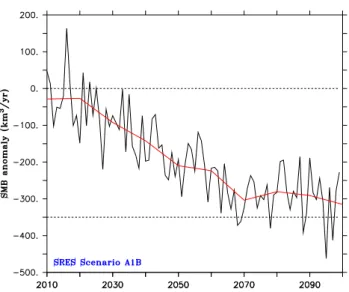
Fig. 7. (a)Time series of SMB anomalies projected by AOGCMs listed in Table 4 fora/b=−1. The anomalies are decadal means and refer to 1970–1999 where the mean SMB rate is estimated to be∼ 350 km3/yr. The anomalies are based on model outputs from the “Climate of the Twentieth Century Experiment” (20C3M) and from the scenario SRES A1B. Finally, the median (50%), the 25% and 75% quartile values among the 24 models, Eq. (7) and the UKMO-HadCM3 time series are plotted in red, dark blue, light blue and green, respectively.
Fig. 8. The 2010–2100 projected SMB anomaly using tem-perature/precipitation anomaly simulated by UKMO-HadCM3 for k=−1. The temperature/precipitation projections from UKMO-HadCM3 are near the ensemble mean and its SMB anomaly pro-jections are at the negative end compared with other models. The 10-yr running mean is shown in red.
For validation purposes, this algorithm was first applied to the ECMWF, NCEP and GHCN time series (1970–1999) by taking a value of −1 for the parameterk. The result-ing estimated SMB time series agree well with those sim-ulated by Hanna08. The correlation coefficient is respec-tively 0.96, 0.97 and 0.86 for a RMSE equals to 32.6, 30.7 and 55.5 km3yr−1. These results should be compared with those listed in Table 3. An alternative to this algorithm (us-ing a fixed value of k) is to directly infer the parameter a and b from the regressions listed in Table 3 (in average, a≃ −60±10 andb≃ +60±10). However, in this case, the RMSE with the SMB time series simulated by Hanna08 is higher.
Figure 6 plots the decadal mean of the JJA temperature and relative precipitation changes for all models listed in Table 4. While the interdecadal variability is very high (particularly for precipitation) and some models are in total disagreement with the others, the models are unanimous in projecting a JJA temperature increase of ∼2.4◦C through the 21st cen-tury. Changes in precipitation are more model-dependent than temperature although the multimodel average gives a small increase of precipitation during the 21st century. The relative precipitation change could be estimated to be∼5% K−1 in connection with the temperature increase, as found by Gregory and Huybrechts (2006). Table 5 summarises the changes projected for the 21st century. These results are in agreement with the projections of the IPCC AR4 (Chris-tensen et al., 2007) for 2090–2099 (compared with 1980– 1999) over a region covering the Greenland (103◦W–10◦W
and 50◦N–85◦N.). Their projections are +2.8 K (+2.1,+3.7) for the JJA temperature and +15% (+12,+20) for the annual relative precipitation. Their values are the median (50%), and 25% and 75% quartile values among 21 AOGCMs.
The ensemble mean of the 24 models used in the 20C3M experiment (see Table 4) gives a mean surface JJA temperature (resp. precipitation) of −1.2±2.7◦C (resp. 530±157 mm) and a trend of+0.02 K◦yr−1(resp. no significant precipitation change) in Region 1 (resp. Region 2) over the reference period 1979–1999. These results are in agreement with observations during 1970–1999, suggesting that the multimodel average is a reliable estimate for the cur-rent climate. In a first approach, we decided to use only re-sults of the ensemble mean for future projections rather than those from a single model. Sophisticated weighting of the various models should be investigated in the future.
The SMB anomaly projection fork=a/b=−1 as well as the cumulated sea level rises equivalent are shown in Fig. 7 and listed in Table 5. The lower SMB anomaly in the 20th century seems to have occurred in 1931 with−300 km3yr−1. This record surface mass loss rate is likely to become com-mon at the end of the 21st century. The summer will prob-ably be much warmer than previously observed during the 20th century, but a predicted increase of precipitation will most likely partly offset the SMB decrease associated with warming. With the SRESA2 experiment, the projected neg-ative SMB anomalies are higher. The sea level rise com-ing from the GrIS SMB change should reach 4±0.5 cm in 2100, which is in full agreement with Huybrechts et al. (2004), Oerlemans et al. (2005) and Meehl et al. (2007). The computation was made by using an area of a world ocean area of 361 million km2. Finally, Table 5 and Fig. 7 show that a warming threshold higher than 2.5 K is required for a zero surface mass balance (i.e. a SMB anomaly reaching
−350 km3/yr in our case), as concluded by Gregory and Huy-brechts (2006).
glacier acceleration as observed by Zwally et al., 2002) and in basal melting currently estimated to be∼300 km3yr−1by
Reeh et al. (1999).
According to Eq. (5) and if we assume that the relative pre-cipitation change is 5% K−1in connection with the
tempera-ture increase (Gregory and Huybrechts, 2006), the ensemble mean of the IPCC AR4 models shows that the projected SMB changes in a near future could be approximated by
1SMB=a 1T
st dev(T20C3M)
+b 1P st dev(P20C3M)
(6)
= ∼(−106±26)1T (7) fork=a/b= −1.0 (−1.5,−0.75). The striking fit between the Eq. (7) plotted in Fig. 7 in light blue and the ensemble mean in red motived us to use Eq. (7) with the IPCC AR4 projections. Following the used SRES scenario, the best es-timates from the IPCC AR4 project a global average surface warming varying between 1.8 and 4 K in 2100 (IPCC, 2007). If we assume that the summer GrIS temperature increase will be equivalent to the global warming, Eq. (7) then estimates 1SMBto vary between−190±47 and−424±104 km3yr−1 in 2100. In particular for the mid-range SRES scenario A1B, the IPCC AR4 (IPCC, 2007) projects a global temperature increase of +2.8 K (+1.7,+4.4) inducing a SMB change of
−297±73 (−180±44,−466±114) km3yr−1in 2100. There-fore, it is very likely that the GrIS SMB should be null or even negative in 2100.
However, ten thousand years would be needed to melt completely the GrIS if the SMB stabilizes near 0 km3yr−1.
Indeed, the total volume of the GrIS is 2.93×10⁶km3 (Bam-ber et al., 2001) and the current mass loss from glacier dis-charge and basal melting is estimated to be∼300 km3yr−1
(Reeh et al., 1999), while some recent observations from the Gravity Recovery and Climate Experiment (GRACE) sug-gest that dynamic mass losses should be much higher within the last five years (Chen et al., 2006; Luthcke et al., 2006; Thomas et al., 2006, Velicogna and Wahr, 2006). However, this simple calculation does not take into account the posi-tive feedbacks from albedo and elevation changes (Ridley et al., 2005) or changes in ice dynamics nor the fact that in a warmer climate the ice sheet will retreat from the coast so that less calving can take place.
5 Discussion and conclusion
Simulations made with MAR (Fettweis, 2007) and by Hanna et al. (2008) reveal a very high correlation between the inter-annual variability of the modelled SMB and the variability of both temperature and precipitation GrIS anomalies. We have derived a multiple-regression relation that has been used with climatological time series to empirically estimate the GrIS SMB since 1900. The SMB changes projected for the end of the 21st century have been derived using the set of exper-iments conducted for the IPCC AR4 (Randall et al., 2007).
The results show that the GrIS surface mass loss in the 1930s is likely to have been more significant than currently due to a combination of very warm and dry years. It is also noted from our results that a mere ten years would be enough to pass from a GrIS growth state to a signifi-cant mass-loss state. Therefore, the SMB changes that are currently occurring, and which are linked to global warm-ing (Fettweis, 2007; Hanna et al., 2008) are not exceptional in the GrIS history. For the near future, the IPCC AR4 mod-els project SMB rates similar to those of the 1930s (i.e. a zero or even negative SMB rate) for the end of the 21st century. That transforms to about 4–5 cm of sea-level rise for the end of this century under SRES scenario A1B. If these rates are confirmed and no significant changes occur in iceberg calv-ing and basal meltcalv-ing, then these rates are not large enough to significantly change the freshwater flux into the Atlantic Ocean.
However, large uncertainties remain indeed in these es-timates due to models/scenarios used as well as parame-ters and hypotheses made in the algorithm to estimate the GrIS SMB anomaly. That is why further investigations are needed. High-resolution simulations made with the MAR model (which explicitly simulates the SMB by incorporat-ing the surface feedbacks) forced at its boundaries by the IPCC AR4 models outputs should yield more comprehen-sive and realistic results although this requires a lot of com-puting time. Moreover, both 2003 and 2006 negative SMB anomalies simulated by MAR resulting from a combination of low precipitation and very high temperatures are equiva-lent to those projected by the AOGCMs on average for the end of the 21st century. This suggests that some AOGCMs could underestimate changes over the GrIS from the global warming.
Acknowledgements. We acknowledge the modelling groups, the Program for Climate Model Diagnosis and Intercomparison (PCMDI) and the WCRP’s Working Group on Coupled Modelling (WGCM) for their roles in making available the WCRP CMIP3 multi-model dataset. Support of this dataset is provided by the Office of Science, US Department of Energy. We thank also the British Atmospheric Data Centre and European Centre for Medium-Range Weather Forecasts (ECMWF) for ECMWF reanal-ysis and operational analreanal-ysis data (used for driving the MAR model and the Hanna et al. (2008) SMB model). Finally, the authors want to thank Wouter Lefebvre for his extremely valuable comments.
References
Bamber, J. L., Layberry, R. L., and Gogineni, S. P.: A new ice thickness and bed data set for the Greenland ice sheet: part I, Measurement, data reduction, and errors, J. Geophys. Res., 106, 33 773–33 780, 2001.
Box, J. E.: Survey of Greenland instrumental temperature records: 1873–2001, Int. J. Climatol., 22, 1829–1847, 2002.
Box, J. E., Bromwich, D. H., and Bai, L.-S.: Greenland ice sheet surface mass balance for 1991–2000: application of Polar MM5 mesoscale model and in-situ data, J. Geophys. Res., 109(D16), D16105, doi:10.1029/2003JD004451, 2004.
Box, J. E. and Cohen, A. E.: Upper-air temperatures around Greenland: 1964–2005, Geophys. Res. Lett., 33, L12706, doi:10.1029/2006GL025723, 2006.
Box, J. E., Bromwich, D. H., Veenhuis, B. A., Bai, L.-S., Stroeve, J. C., Rogers, J. C., Steffen, K., Haran, T., and Wang, S.-H.: Green-land ice sheet surface mass balance variability (1988–2004) from calibrated Polar MM5 output, J. Climate, 19(12), 2783–2800, 2006.
Cappelen, J., Jorgensen, B. V., Laursen, E. V., Stannius, L. S., and Thomsen, R. S.: The observed climate of Greenland, 1958–99 – with climatological standard normals, 1961–1990, Tech. Rep. 00-18, 152 pp., Danish Meteorological Institute, Copenhagen, 2001.
Chen J. L., Wilson, C. R., and Tapley, B. D.: Satellite Gravity Mea-surements Confirm Accelerated Melting of Greenland Ice Sheet, Science, 313, 1958–1960, doi:10.1126/science.1129007, 2006. Chylek, P., Dubey, M. K., and Lesins, G.: Greenland warming of
1920–1930 and 1995–2005, Geophys. Res. Lett., 33, L11707, doi:10.1029/2006GL026510, 2006.
Chylek, P., McCabe, M., Dubey, M. K., and Dozier, J.: Re-mote sensing of Greenland ice sheet using multispectral near-infrared and visible radiances, J. Geophys. Res., 112, D24S20, doi:10.1029/2007JD008742, 2007.
Christensen, J. H., Hewitson, B., Busuioc, A., Chen, A., Gao, X., Held, I., Jones, R., Kolli, R. K., Kwon, W.-T., Laprise, R., Mag-ana Rueda, V., Mearns, L., Menendez, C. G., Risnen, J., Rinke, A., Sarr, A., and Whetton, P.: Regional Climate Projections, in: Climate Change 2007: The Physical Science Basis. Contribution of Working Group I to the Fourth Assessment Report of the In-tergovernmental Panel on Climate Change, edited by: Solomon, S., Qin, D., Manning, M., Chen, Z., Marquis, M., Averyt, K. B., Tignor, M., and Miller, H. L., Cambridge University Press, Cambridge, United Kingdom and New York, NY, USA, 2007. Christy, J. R., Spencer, R. W., and Braswell, W. D.: MSU
Tropo-spheric temperatures: Data set construction and radiosonde com-parisons, J. Atmos. Ocean. Tech., 17, 1153–1170, 2000. Cuffey, K. M. and Marshall, S. J.: Substantial contribution to sea
level rise during the last interglacial from the Greenland ice sheet, Nature, 404, 591–594, 2000.
Dai, A., Fung, I. Y., and Del Genio, A. D.: Surface observed global land precipitation variations during 1900–1988, J. Climate, 10, 2943–2962, 1997.
Fettweis, X., Gall´ee, H., Lefebre, L., and van Ypersele, J.-P.: Greenland surface mass balance simulated by a regional climate model and comparison with satellite derived data in 1990–1991, Clim. Dynam., 24, 623–640, doi:10.1007/s00382-005-0010-y, 2005.
Fettweis, X., van Ypersele, J.-P., Gall´ee, H., Lefebre, F., and
Lefeb-vre, W.: The 1979–2005 Greenland ice sheet melt extent from passive microwave data using an improved version of the melt retrieval XPGR algorithm, Geophys. Res. Lett., 34, L05502, doi:10.1029/2006GL028787, 2007.
Fettweis, X.: Reconstruction of the 1979–2006 Greenland ice sheet surface mass balance using the regional climate model MAR, The Cryosphere, 1, 21–40, 2007.
Gregory, J., Dixon, K., Stouffer, R. J., Weaver, A., Driesschaert, E., Eby, M., Fichefet, T., Hasumi, H., Hu, A., Jungclaus, J., Kamenkovich, I., Levermann, A., Montoya, M., Murakami, S., Nawrath, S., Oka, A., Solokov, A., and Thorpe, R.: A model intercomparison of changes in the Atlantic thermohaline circu-lation in response to increasing atmospheric concentration, Geo-phys. Res. Lett., 32, L12703, doi:10.1029/2005GL023209, 2005. Gregory, J. and Huybrechts, P.: Ice-sheet contributions to future
sea-level change, Philos. T. R. Soc. A, 364, 1709–1731, 2006. Hanna, E., Box, J., and Huybrechts, P.: Greenland Ice Sheet mass
balance, Arctic Report Card 2007, update to State of Arctic Report 2006, NOAA, available at http://www.arctic.noaa.gov/ reportcard/, 2007.
Hanna, E., Huybrechts, P., Steffen, K. , Cappelen, J., Huff, R., Shu-man, C., Irvine-Fynn, T., Wise, S., and Griffiths, M.: Increased runoff from melt from the Greenland Ice Sheet: a response to global warming, J. Climate, 21, 331–341, 2008.
Huybrechts, P., Gregory, J., Janssens, I., and Wild, M.: Modelling Antarctic and Greenland volume changes dur-ing the 20th and 21st centuries forced by GCM time slice integrations, Global Planet. Change, 42, 83–105, doi:10.1016/j.gloplacha.2003.11.011, 2004.
IPCC, 2007: in: Climate Change 2007: The Physical Science Basis. Contribution of Working Group I to the Fourth Assessment Re-port of the Intergovernmental Panel on Climate Change, edited by: Solomon, S., Qin, D., Manning, M., Chen, Z., Marquis, M., Averyt, K. B., Tignor, M., and Miller, H. L., Cambridge Uni-versity Press, Cambridge, United Kingdom and New York, NY, USA, 2007.
Kalnay, E., Kanamitsu, M., Kistler, R., Collins, W., Deaven, D., Gandin, L., Iredell, M., Saha, S., White, G., Woollen, J., Zhu, Y., Leetmaa, A., Reynolds, B., Chelliah, M., Ebisuzaki, W., Higgins, W., Janowiak, J., Mo, K., Ropelewski, C., Wang, J., Jenne, R., and Joseph, D.: The NCEP/NCAR 40-Year Reanalysis Project, B. Am. Meteorol. Soc., 77, 437–471, 1996.
Luthcke, S. B., Zwally, H. J., Abdalati, W., Rowlands, D. D., Ray, R. D., Nerem, R. S., Lemoine, F. G., McCarthy, J. J., and Chinn, D. S.: Recent Greenland Ice Mass Loss by Drainage System from Satellite Gravity Observations, Science, 314(5803), 1286, doi:10.1126/science.1130776, 2006.
Meehl, G. A., Stocker, T. F., Collins, W. D., Friedlingstein, P., Gaye, A. T., Gregory, J. M., Kitoh, A., Knutti, R., Murphy, J. M., Noda, A., Raper, S. C. B., Watterson, I. G., Weaver, A. J., and Zhao, Z.-C.: Global Climate Projections, in: Climate Change 2007: The Physical Science Basis. Contribution of Working Group I to the Fourth Assessment Report of the Intergovernmental Panel on Climate Change, edited by: Solomon, S., Qin, D., Manning, M., Chen, Z., Marquis, M., Averyt, K. B., Tignor, M., and Miller, H. L., Cambridge University Press, Cambridge, United Kingdom and New York, NY, USA, 2007.
high-resolution grids, Int. J. Climatol., 25, 693–712, 2005. Nakicenovic, N., Alcamo, J., Davis, G., et al.: Special Report on
Emissions Scenarios: A Special Report of Working Group III of the Intergovernmental Panel on Climate Change, Cambridge University Press, Cambridge, UK, 599 pp., available online at: http://www.grida.no/climate/ipcc/emission, 2000.
Peterson, T. C. and Vose, R. S.: An overview of the Global Histor-ical Climatology Network temperature database, B. Am. Meteo-rol. Soc., 78(12), 2837–2849, 1997.
Oerlemans, J., Bassford, R. P., Chapman, W., Dowdeswell, J. A., Glazovsky, A. F., Hagen, J. O., Melvold, K., de Wildt, M. R. and van de Wal, R. S. W.: Estimating the contribution from Arc-tic glaciers to sea-level change in the next hundred years, Ann. Glaciol, 42, 230–236, 2005.
Rahmstorf, S., Crucifix, M., Ganopolski, A., Goosse, H., Ka-menkovich, I., Knutti, R., Lohmann, G., Marsh, R., Mysak, L. A., Wang, Z., and Weaver, A. J.: Thermohaline circulation hys-teresis: A model intercomparison, Geophys. Res. Lett., 32(23), L23605, doi:10.1029/2005GL023655, 2005.
Randall, D. A., Wood, R. A., Bony, S., Colman, R., Fichefet, T., Fyfe, J., Kattsov, V., Pitman, A., Shukla, J., Srinivasan, J., Stouf-fer, R. J., Sumi, A., and Taylor, K. E.: Climate Models and Their Evaluation, in: Climate Change 2007: The Physical Science Basis. Contribution of Working Group I to the Fourth Assess-ment Report of the IntergovernAssess-mental Panel on Climate Change, edited by: Solomon, S., Qin, D., Manning, M., Chen, Z., Mar-quis, M., Averyt, K. B., Tignor, M., and Miller, H. L., Cambridge University Press, Cambridge, United Kingdom and New York, NY, USA, 2007.
Reeh, N., Mayer, C., Miller, H., Thomson, H. H., and Weidick, A.: Present and past climate control on fjord glaciations in Green-land: Implications for IRD-deposition in the sea, Geophys. Res. Lett., 26, 1039–1042, 1999.
Ridley, J., Huybrechts, P., Gregory, J. M., and Lowe, J.: Elimination of the Greenland ice sheet in a high-CO2 climate, J. Climate, 18(17), 3409–3427, 2005.
Rignot, E. and Kanagaratnam, P.: Changes in the Velocity Struc-ture of the Greenland Ice Sheet, Science, 311, 986–990, doi: 10.1126/science.112138, 2006.
Swingedouw, D., Braconnot, P., and Marti, O.: Sensitivity of the Atlantic Meridional Overturning Circulation to the melting from northern glaciers in climate change experiments, Geophys. Res. Lett., 33, L07711, doi:10.1029/2006GL025765, 2006.
Thomas, R., Frederick, E., Krabill, W., Manizade, S., and Martin, C.: Progressive increase in ice loss from Greenland, Geophys. Res. Lett., 33, L10503, doi:10.1029/2006GL026075, 2006. Uppala, S. M., Kallberg, P. W., Simmons, A. J., Andrae, U., da
Costa Bechtold, V., Fiorino, M., Gibson, J. K., Haseler, J., Her-nandez, A., Kelly, G. A., Li, X., Onogi, K., Saarinen, S., Sokka, N., Allan, R. P., Andersson, E., Arpe, K., Balmaseda, M. A., Beljaars, A. C. M., van de Berg, L., Bidlot, J., Bormann, N., Caires, S., Chevallier, F., Dethof, A., Dragosavac, M., Fisher, M., Fuentes, M., Hagemann, S., Holm, E., Hoskins, B., Isaksen, L., Janssen, P. A. E. M., Jenne, R., McNally, A. P., Mahfouf, J.-F., Morcrette, J.-J., Rayner, N. A., Saunders, R. W., Simon, P., Sterl, A., Trenberth, K. E., Untch, A.,Vasiljevic, D., Viterbo, P., and Woollen, J.: The ECMWF re-analysis, Q. J. Roy. Meteor. Soc., 131, 2961–3012, doi:10.1256/qj.04.176, 2005.
Velicogna, I. and J. Wahr: Measurements of Time-Variable Gravity Show Mass Loss in Antarctica, Science, 311(5768), 1754–1756, 2006.
Vinther, B. M., Andersen, K. K., Jones, P. D., Briffa, K. R., and Cappelen, J.: Extending Greenland temperature records into the late eighteenth century, J. Geophys. Res., 111, D11105, doi:10.1029/2005JD006810, 2006.