Electricity Load Forecasting based on Framelet Neural Network Technique

American Journal of Applied Sciences 6 (5): 970-973, 2009 ISSN 1546-9239

© 2009 Science Publications

970

Electricity Load Forecasting based on Framelet Neural Network Technique

Mohammed K. Abd

Department of Electrical and Electronic Engineering, University of Technology, Baghdad, Iraq

Abstract: Load forecasting is very essential to the operation of electricity companies. It enhances the energy-efficient and reliable operation of a power system. This study shows Electricity Load Forecasting modeling based on Framelet Neural Network Technique (FNN) for Baghdad City. Framelet technique is implemented to the time series data, decomposing the data into number of Framelet coefficient signals. The decomposed signals are then fed into neural network for training. To obtain the predict forecast, the outputs from the neural network are recombined using the same Framelet technique. The simulation results showed that the model was capable of producing a reasonable forecasting accuracy in short term load forecast.

Key words: Load forecasting, framelet, neural network, series time data.

INTRODUCTION

Many power systems not only are being pushed to their limits to meet their customers’ demands, but also spend a lot of resources in their operation scheduling. System security is becoming an ever more important issue in modern electrical power systems. It is known for all that electrical energy cannot be stored efficiently, due to this fact that the electrical load could be controlled by utilities only to a very small extent, the forecasting of load demand data forms an important component in planning generation schedules in a power system.

The short term load forecast is to predict future electricity demands based on historical data and other information such as temperature. Time series forecast is traditionally based on linear models e.g., Auto-regressive Moving Average (ARMA) models[2], have been used for Load Forecasting[4]. These models are straight for implementation but fail to give satisfactory results when dealing with nonlinear, non-stationary time series. The solution to that is Neural Network as supervised models have been used to deal with the nonlinearity and non-stationary in electricity load prediction and have produced good and satisfactory results[1,3,5], for their approximation ability for nonlinear mapping and generalization. However, it suffers from the problem of obtaining monolithic global models for a time series. This introduced the multi-resolution decomposition techniques such as Framelet transform approach. Framelet transforms provide a useful decomposition of the time series, in terms of both time and frequency. They have been used effectively for image compression, noise removal, object detection and

large-scale structure analysis, among other applications[5].

For this study, combining the learning capabilities of neural networks and time series techniques and using Framelet decomposition technique to explore more details of the time series signals. A multi-layer perception neural network is applied to each decomposed series to predict the time series. We will study neural network models combined with Framelet transformed data, and show how useful information can be captured on various time scales.

Framelet technique: Framelet are very similar to wavelets but have some important differences. In particular, whereas wavelets have an associated scaling function Ф(t) and wavelet function ψ(t), framelets have one scaling function Ф(t) and two wavelet functions

ψ1(t) and ψ2(t) .

The scaling function Ф(t) and the wavelets ψ1(t) and ψ2(t) are defined through these equations by the low-pass (scaling) filter h0(n) and the two high-pass

(wavelet) filters h1(n) and h2(n). Let Фk (t)= Ф(t-n) and:

ψi,j,k(t)= ψi (2j t-k) for i=1,2 (1)

Any function f(t) could be written as a series expansion in terms of the scaling function and wavelets by[6]:

k 1 1, j,k 2 2, j,k

k j 0 k

f (t) c(k) (t) d ( j, k) (t) d ( j, k) (t)

∞ ∞ ∞

=−∞ = =−∞

=

∑

∑ ∑

Where:

k

Am. J. Applied Sci., 6 (5): 970-973, 2009

971

i i, j, k

d ( j, k)=

∫

In this expansion, the first summation gives a function that is a low resolution or coarse approximation of f(t) at scale j = 0. For each increasing j in the second summation, a higher or finer resolution function is added, which adds increasing details.

A Framelet base is employed in the hidden layer of FNN rather than a sigmoid function, which discriminates it from general back propagation neural networks[7,8].

The training algorithm of FNN is elucidated as following steps:

Step 1: Data acquisition: The output response voltage signals of test point are sampled in terms of the SY running under different input step voltage. Then optimal features for training neural networks are obtained by wavelet decomposing coefficients and normalization

Step 2: Select the parameters of wavelet neural network: The dimension of fault feature vectors and the circuit fault pattern determines the number of input node and output node. The output number is equal to the number of fault classes, while input number is equal to the dimension of feature vectors. The number of neurons on hidden layer is set greater or equal to M+ +N a, where M and N is the node number of input layer and output layer and is set 1~10

Step 3: Training of wavelet neural network: The different input step voltage vectors, as input vectors of training pattern, are used to train the wavelet neural network. The output vectors reflect the states of SY. The gradient descent algorithm is employed to minimize the error function so as to adjust the weights of network. The error function is:

p

p j

p

j j

p 1 j 1 1

E y (t) y (t)

2

∗

= =

 

=  − 

 

∑∑

where P is the total number of training patterns

p *

j

y (t)and

p j

y (t) are the desired and real output

associated with the jth feature for the pth neuron.

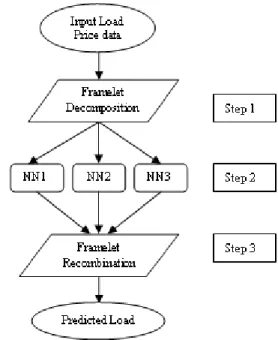
Fig. 1: Flowchart of the forecast based on FNN MATERIALS AND METHODS

Electricity load forecasting based on FNN: The block diagram of the forecasting model principle based on framelet neural network is given in Fig. 1. The data used in the model to train neural networks are historical electricity load and pricing data. As for the data process tool Framelet Technique is used in the model.

The model consists of three stages:

Step 1: Data Pre-processing Step 2: Data Prediction Step 3: Data Post-processing

The preliminary forecast model has three main stages. This is illustrated in flowchart below;

Model validation: The model is evaluated based on it prediction errors. A successful model would give an accurate time-series forecast. The performance of the model is hence measured using the Mean Absolute Percentage Error (MAPE) which is defined as:

Absolute Percentage Error (APE), which is defined as:

Actual(i) Forecast(i)

APE(%) *100

Actual(i)

−

= (5)

Am. J. Applied Sci., 6 (5): 970-973, 2009

972

X

i 1

Actual(i) Forecast (i) 1

MAPE(%) *100

x = Actual(i)

−

=

∑

Where:

X = The total number of hours predicted Actual(i) = The actual load for the hour i, Forecast(i) = The predicted load for the hour i.

RESULTS AND DISCUSSION

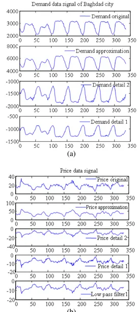
Model simulation result: The proposed model is tested with two sets of historical data containing the electricity load and price data of Baghdad City as shown in Fig. 2, on a half-hourly basis, 1-7 June 2004.

Price is only used with load to form a particular time-series pattern as the inputs for training the neural networks, the model output was only the predicated electricity load and tested with a number of different values of hidden neurons, however no significant changes are observed with the predicted results. Therefore for this study, the number of hidden neurons is set to two.

The model consists of three steps:

Step one: Demand and price historical time-series data of Baghdad City are decomposed at resolution level 2 as shown in Fig. 3 (A and B) respectively .

Step two: As depicted in forecast model, three neural networks were created for the forecast model-one for the approximation series and one for each of the two Framelet coefficient series. The neural networks were trained with 1 day (48 points), 2 days (98 points),

Rashdiy Jameela Thawra Muthanna Farabi

(132/33)

(132/33)

Mansoor New Jadiriy Sarrafya

Meedan

Khadmiya Maarry

Tagi Hurriya Jamiaa Yarmok Jazair Daur

132 kV

Baghdad West (400/132) Baghdad West (400/132)

Khazali Waziriya

New Bag.

Bag. South Qusaiba 132 kV

Fig. 2: Distribution network structure of Baghdad city

(a)

(b)

Fig. 3: Decomposition of Baghdad city (a)Demand series data(b) Price series data

0 5 10 15 20 25 30 35 40 45 50

2200 2300 2400 2500 2600 2700 2800 2900 3000 3100

Mean absolute error = 0.018394 Actual

Forecasted

Am. J. Applied Sci., 6 (5): 970-973, 2009

973

0 50 100 150 2000

2200 2400 2600 2800 3000 3200

3400 Mean absolute error = 0.018651 Actual

Forecasted

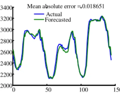
Fig. 5: Load forecasted for 3 days (144 points)

0 50 100 150 200 250 2000

2200 2400 2600 2800 3000 3200 3400

Mean absolute error = 0.017976 Actual Forecasted

Fig. 6: Load forecasted for 5 days (240 points)

0 50 100 150 200 250 300 350 2000

2200 2400 2600 2800 3000 3200 3400

Mean absolute error = 0.018465 Actual Forecasted

Fig. 7: Load forecasted for 7 days (336 points)

Table 1: Summary of MAPEs

No. of forecasted points Mean absolute error (%)

48 (1 days) 0.018394

96 (2 days) 0.019877

144 (3 days) 0.018651

192 (4 days) 0.018105

240 (5 days) 0.017976

288 (6 days) 0.018313

336 (7 days) 0.018465

3 days (144 points), 4 days (192 points), 5 days (240 points), 6 days (288 points) and 7 days (336 points) of combined load and price data for fifty cycles. Step three: The performance of the forecast model was evaluated and the results are as shown in Fig.4-7. Model validation: The performance of the proposed model is measured by the MAPE using Eq. 6. These

MAPEs were recorded in Table 1. The MAPE calculated is less than 0.019877% of Baghdad city.

CONCLUSION

This study proposed a LFFNN model with a high forecasting accuracy. The FNN has been successfully implemented in the model. The results obtained in this work confirm the applicability as well as the efficiency of neural networks in short-term load forecasting. The implementation of FNN has reasonably enhanced the learning capability of the NNs in the model, thus minimizing their training frequencies as shown in the simulations. The neural network was able to determine the nonlinear relationship that exists between the historical load data supplied to it during the training phase and on that basis, and make a prediction of what the load would be in the next and the use of FNN (as the data processing tool) for the proposed model have been a success.

REFERENCES

1. Chow, T.W.S. and C.T. Leung, 1996. Neural networks based short term load forecasting using weather compensation. IEEE Trans. Power Syst., 11: 1736-1742. DOI: 10.1109/59.544636

2. Francisco, N.J. and C. Javier, et al., 2002. Forecasting next-day electricity prices by times series models. IEEE Trans. Power Syst., 17: 342-348.

DOI:10.1109/TPWRS.2002.1007902

3. Hipert, H.B. and C.E. Pedreira, et al., 2001. Neural-networks for short term load forecasting: A review and evaluation. IEEE Trans. Power Sys., 16: 44-55. DOI:10.1109/59.910780

4. Moghram, I. and R. Saifur, 1989. Analysis and evaluation of five short-term load forecasting techniques. IEEE Trans. Power Syst., 4: 1484-1491. DOI:10.1109/59.41700

5. Khtanzad, A., R. Afkhami-Rohani and D.J. Maratukulam, 1998. ANN STLF artificial neural network short-term load forecaster-generation three. IEEE Trans. Power Syst., 13: 1423-1422. 6. Selesnick, I.W., 2001. Smooth wavelet tight frames

with zero moments. Applied Comput. Harmonic Anal. 10: 163-181.DOI: 10.1006/acha.2000.0332 7. Kingsbury, N.G., 1998. The dual-tree complex

wavelet transform: A new technique for shift invariance and directional filters. Proceedings of the 8th IEEE DSP Workshop’ 98, Utah, pp: 319-322. http://citeseerx.ist.psu.edu/viewdoc/summary?doi= 10.1.1.51.1213

8. Al-Taai, H.N., 2008. A Novel fast computing framelet coefficients method. Am. J. Appli. Sci., 5: 1522-1527.