www.atmos-chem-phys.net/12/11819/2012/ doi:10.5194/acp-12-11819-2012
© Author(s) 2012. CC Attribution 3.0 License.
Chemistry
and Physics
Implications of all season Arctic sea-ice anomalies
on the stratosphere
D. Cai, M. Dameris, H. Garny, and T. Runde
Deutsches Zentrum f¨ur Luft- und Raumfahrt, Institut f¨ur Physik der Atmosph¨are, Oberpfaffenhofen, Germany
Correspondence to:D. Cai ([email protected])
Received: 13 February 2012 – Published in Atmos. Chem. Phys. Discuss.: 15 May 2012 Revised: 28 November 2012 – Accepted: 4 December 2012 – Published: 17 December 2012
Abstract.In this study the impact of a substantially reduced Arctic sea-ice cover on the lower and middle stratosphere is investigated. For this purpose two simulations with fixed boundary conditions (the so-called time-slice mode) were performed with a Chemistry-Climate Model. A reference time-slice with boundary conditions representing the year 2000 is compared to a second sensitivity simulation in which the boundary conditions are identical apart from the polar sea-ice cover, which is set to represent the years 2089–2099. Three features of Arctic air temperature response have been identified which are discussed in detail. Firstly, tro-pospheric mean polar temperatures increase up to 7 K dur-ing winter. This warmdur-ing is primarily driven by changes in outgoing long-wave radiation. The tropospheric response (e.g. geopotential height anomaly) is in reasonable agree-ment with similar studies dealing with Arctic sea-ice de-crease and the consequences on the troposphere. Secondly, temperatures decrease significantly in the summer strato-sphere caused by a decline in outgoing short-wave radiation, accompanied by a slight increase of ozone mixing ratios. Thirdly, there are short periods of statistical significant tem-perature anomalies in the winter stratosphere probably driven by modified planetary wave activity, but generally there is no clear stratospheric response. The Arctic Oscillation (AO)-index, which is related to the troposphere–stratosphere cou-pling favours a more neutral state during winter. The only clear stratospheric response can be shown during Novem-ber. Significant changes in Arctic temperature, meridional eddy heat fluxes and the Arctic Oscillation (AO)-index are detected.
In this study the overall stratospheric response to the pre-scribed sea-ice anomaly is small compared to the tropo-spheric changes.
1 Introduction
Arctic sea-ice cover has considerably declined in the current century and further decreases are predicted by general cir-culation models in response to increasing greenhouse gas (GHG) concentrations (IPCC, 2007). Clear loss of Arctic sea-ice has been observed with the largest rate of decline in late summer months (e.g. Deser and Teng, 2008). Climate models predict a nearly ice-free summer in the Arctic within the coming 15–50 yr (e.g. Holland et al., 2006). But it must be taken into account that observed sea-ice reduction in re-cent years was much stronger than predicted by climate mod-els, (e.g. the IPCC AR4 models; Wu et al., 2006; Stroeve et al., 2007; Maslanik et al., 2007; Holland et al., 2007; see also Fig. 1 in Scinocca), offering the possibility of a quicker disappearance of Arctic sea-ice in summer and autumn.
Observational (e.g. Francis et al., 2009) as well as nu-merical modeling studies (see Budikova, 2009 for a compre-hensive review) have suggested that sea-ice anomalies have a pronounced spatial and temporal impact on the overlying atmosphere. Numerous investigations have been performed pointing out significant changes in tropospheric conditions (e.g. storm-track distribution and strength over mid- and high latitudes, air temperature, precipitation, etc.; Magnusdottir et al., 2004; Deser et al., 2004, 2010; Alexander et al., 2004; Singarayer et al., 2006; Seierstad and Bader, 2009; Orsolini et al., 2012).
is intimately coupled to the variability of the strength of the stratospheric polar vortex (e.g. Thompson and Wallace, 1998; Schnadt and Dameris, 2003; Wang and Ikeda, 2000; Black, 2002; Baldwin and Dunkerton, 2005; Scaife et al., 2005; Rind et al., 2005): a positive AO-index corresponds to an anomalously strong polar vortex, while an anomalously weak polar vortex is found when the AO-index is negative.
Alterations in tropospheric conditions due to sea-ice re-treat (e.g. changes in meridional temperature gradient or storm-track distribution and strength) could affect planetary wave forcing. Since planetary waves play an major role in the troposphere–stratosphere coupling a potential stratospheric response can be expected.
Scinocca et al. (2009) also raised the issue of stratospheric response to Arctic sea-ice reduction. They studied the sensi-tivity of Northern Hemisphere polar ozone recovery to com-plete sea-ice loss during summer. Based on long-term nu-merical simulations with the Canadian Middle Atmosphere Model (CMAM), i.e. a Chemistry-Climate Model (CCM) coupled to an ocean general circulation model, they found significant surface warming and stratospheric cooling in the North Polar region during March. Scinocca and colleagues showed that circulation changes in the troposphere are simi-lar to those found in other studies (see above) and that plane-tary wave forcing of the stratosphere is reduced in response to the sea-ice loss. Consequently, downwelling over the North Polar region in March was reduced and therefore (dynam-ical) cooling over the polar region together with a reduced downward flux of ozone into the polar middle stratosphere was leading to less ozone.
This paper aims to identify the possible impacts of a sea-sonally ice-free Arctic Ocean on stratospheric dynamics dur-ing all seasons and to investigate in more detail the cause and effect relationship of the stratospheric response to the pre-scribed sea-ice modifications. The paper is organised in the following way: the next section provides a brief repetition of the most important features of the CCM E39CA which is used for this study and a comprehensive description of the model set-up chosen for the numerical simulations. In Sect. 3 the results of analyses are presented and discussed. At first the Arctic tropospheric and stratospheric response is shown. Stratospheric results are separated in winter and sum-mer response. Then tropospheric–stratospheric interaction is analysed with the help of meridional eddy heat flux and
AO-latitude-longitude grid. The vertical partitioning of the model extent from surface to 10 hPa occurs in 39 layers us-ing sigma-pressure coordinates. E39CA is based on spec-tral general circulation model ECHAM4.L39(DLR) (Land et al., 1999), coupled to the chemistry-module CHEM (Steil et al., 1998). The model uses the fully Lagrangian advec-tion scheme ATTILA (Reithmeier and Sausen, 2002). More details of E39CA can be found in Stenke et al. (2008) and Stenke et al. (2009). The model version E39CA as used here was part in the extensive inter-model comparison and eval-uation project CCMVal-2 (SPARC CCM Val et al., 2010). E39CA, as most CCMs has its strengths and weaknesses (e.g. E39CA reproduces well short- and long-term fluctua-tion of stratospheric ozone but polar stratosphere has a cold bias). Nevertheless E39CA performs well in representing tro-pospheric dynamics and the behaviour of the upper tropo-sphere, lower stratosphere region including the coupling of both layers (Gettelman et al., 2010; Hegglin et al., 2010). Moreover E39CA is sufficiently able to reproduce the main feature of stratospheric dynamics and chemistry. This all are necessary properties to carry out this study.
2.2 Simulation set-ups
To identify the atmospheric response of Arctic sea-ice con-tent (SIC) two simulations were conducted in the so-called timeslice mode, i.e. the equilibrium climate state of one pe-riod is simulated by varying only the intra-annual and keep-ing the inter-annual boundary conditions constant. Each sim-ulation was integrated over a 20-yr period following a 5 yr spin-up.
Apart from the lower boundary conditions the setup for the “perturbed” simulation run (NO-ICE) is identical to REF. In a first step we remove the polar sea-ice distribution and utilise “future” conditions instead. The “future” conditions were derived by the climatological mean of the annual cycle of HadGEM1 simulation over the period of 2089–2098 (sce-nario A1B). Since the “future” sea-ice cap is much smaller than before gaps arises between areas covered by ice and the SST field from 1995–2004. These gaps represented by grid points were refilled as follows.
The neighboring grid points of each ”empty” grid point are checked for available “old” SST values. A linear inter-polation of all available “old” SST values is then applied. If no “old” SST data is found the “future” SST is implemented. To avoid discontinuities in the SSTs field, regions containing “future” SSTs were smoothed by interpolation in the latitu-dinal direction.
This approach is certainly only one among a various num-ber of methods to implement SIC anomalies, which also con-tributes to the experimental uncertainties. The discussion of results has to regard this point (see in particular Sects. 3.1 and 3.6)
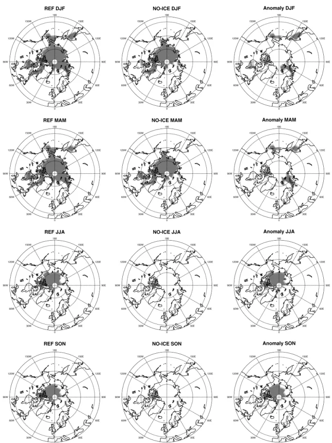
Figure 1 shows the prescribed SIC in terms of seasonal means. In REF, Arctic SIC maximises in its extend during DJF and MAM. Sea-ice covers the whole Arctic Ocean and big parts of its surrounding oceans. In the course of summer the ice surface reduces continuously and reaches its mini-mum in autumn, but sea-ice is still left in the area of the cen-ter of the Arctic Ocean. The situation in NO-ICE is funda-mentally different. In contrast to REF most of the surround-ing Arctic waters are ice-free, like the Bersurround-ing Strait or Sea of Okhotsk in the North-east Pacific. Especially in summer, sea-ice is almost completely removed.
3 Results
The following investigations are based on comparisons be-tween the two E39CA time-slice simulations REF and NO-ICE which differ from each other only in the prescribed Arc-tic sea-ice distributions. Differences in SIC are largest in summer and autumn months (Fig. 1). The results presented here focus on the stratospheric response to the predefined lower boundary conditions over the whole year.
Seasonal zonal means of stratospheric fields like tempera-ture, zonal wind and ozone concentration derived from REF and NO-ICE yield statistically significant differences partic-ularly in high northern latitudes (not shown). Therefore, the subsequent analyses concentrate on middle to high latitudes of the Northern Hemisphere. Figure 2 shows climatologi-cal mean temperature differences for the North Polar region (60◦–90◦N) as derived from the two simulations (i.e.
NO-ICE minus REF). The climatological means are based on 20-years of daily model data in each case (see Sect. 2.2). There are three features of interest which will be discussed in the
following: (A) the Arctic tropospheric temperature changes, (B) the Arctic stratospheric temperature response in summer, and (C) the Arctic stratospheric temperature response in win-ter and early spring.
3.1 Arctic tropospheric response (area A)
Before the stratospheric response is discussed in detail (sub-sequent subsections), the strength and the seasonal behaviour of tropospheric temperature changes in the Arctic are com-pared to respective values mentioned in some of the previous studies presented in Sect. 1. This allows quantifying of the direct tropospheric temperature response in E39CA to the applied sea-ice perturbation in comparison to other similar investigations (see Sect. 2.2).
In contrast to the anomalies of Arctic sea-ice content (NO-ICE minus REF) (Fig. 1), the temperature response in this study is most prominent during late autumn to early spring. Especially in early winter (November, December) tempera-ture changes are large which is in agreement with the sea-sonal structure of recent (1979–2008) Arctic-mean tempera-ture trends derived from a reanalysis ensemble provided by Screen et al. (2012).
Fig. 2.Daily Arctic temperature response (NO-ICE−REF). Fol-lowing student t-test shaded areas are significant at a 95 % level. Labeled ticks mark mid of the month.
December when a robust temperature signal is found up to about 4 km.
In response to the seasonal changes in ocean-atmosphere temperature gradient the differences in outgoing long-wave (LW) radiative flux at the surface is largest in periods of greatest temperature anomalies (Fig. 7b). From August to February there is a marked increase of LW upward radia-tive flux. In the course of early winter the difference between NO-ICE and REF reaches a maximum of 31 W m−2whereas
during summer differences are only in the order of 2.5 to 3 W m−2. Consistent to Alexander et al. (2004) maximum
values of LW outgoing radiation response can locally exceed 100 W m−2(not shown).
The E39CA results presented in this subsection indicates that the overall temporal and spatial response of the lower troposphere to prescribed Arctic SST/SIC perturbations are reasonable, i.e. they are mostly in accordance with assess-ments derived from similar sensitivity studies (e.g. Overland et al., 2008; Francis et al., 2009; Scinocca et al., 2009; Or-solini et al., 2012). The uncertainty introduced by the artifi-cal choice of SSTs and SIC will be discussed in more detail in Sect. 3.6.
3.2 Arctic summer stratospheric response (area B)
In the stratosphere above about 23 km a statistically signifi-cant cooling of approx. 0.5 K is identified from the beginning of July to the end of August (Fig. 2). This cooling is likely related to changes in short-wave (SW) radiation (Fig. 7a) which are strongest from May to August. As prescribed, dur-ing summer the greatest changes in Arctic sea-ice content occur and hence largest changes in surface albedo are at that time. A great extent of highly reflecting sea-ice is replaced by comparable dark open water. So the largest difference of SW reflecting radiation of 21 W m−2near the surface of the North
Polar region is found in July. As a possible consequence of the reduction of reflected SW radiation during late spring and summer the stratosphere in NO-ICE is generally colder than in REF. The statistical insignificance of the negative
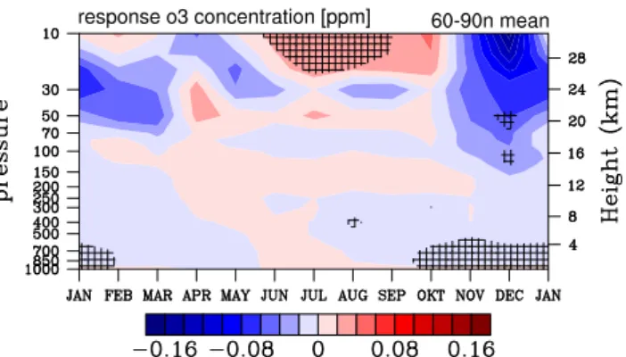
strato-Fig. 3. Monthly mean Arctic ozone mixing ratio response (NO-ICE−REF). Following student t-test shaded areas are significant at a 95 % level.
spheric temperature response in late spring/early summer and early fall (which has the same order of magnitude) is caused by enhanced inter-annual variability in these seasons.
Obviously higher stratospheric ozone mixing ratios of up to 40 ppb above about 24 km are detected in NO-ICE be-tween June and August (Fig. 3). Although the change of ozone mixing ratios are relatively small (i.e. about 1 %) it is statistically significant since the internal variability during summer is very low. In principle the positive ozone signal is contemporaneous to the negative one of stratospheric tem-perature. This connection is explained by the well understood temperature dependencies of ozone destroying chemical re-actions at altitudes above around 25 km. Ozone loss slows down significantly when temperatures are lower (e.g. Haigh and Pyle, 1982; Dameris, 2010; Chapt. 4 in WMO, 2011), explaining the gain of ozone during the period of decreased temperatures in the summer stratosphere.
3.3 Arctic extended-winter (November–March) stratospheric response (area C)
Figure 2 displays a prominent and statistically significant cooling of the stratosphere in the NO-ICE simulation aris-ing in the second half of November (significance level 95 %) which continues with smaller values until mid December. The maximum difference between REF and NO-ICE is
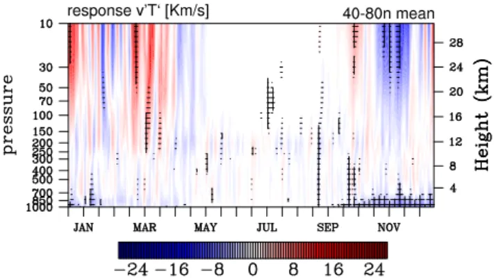
Fig. 4.Dailyv′T′response (NO-ICE−REF) averaged from 40◦–
80◦N. Following student t-test shaded areas are significant at a 95 %
level. Labeled ticks mark mid of the month.
Fig. 5. Stationary component of daily v′T′ response
(NO-ICE−REF) averaged from 40◦–80◦N. Following student t-test
shaded areas are significant at a 95 % level. Labeled ticks mark mid of the month.
the year to early spring ranges from−1.5 to 1.5 K. The mid
winter and early spring months (December–March) response in the North Polar region is only significant for the 75 % level due to the high internal variability (not shown). Nevertheless, in the following we explore in more detail potential connec-tions of changes in Northern atmospheric circulation patterns and corresponding dynamical feedbacks to the stratosphere. 3.4 Meridional heat fluxes
The zonal mean of the meridional eddy heat flux (v′T′) in
middle latitudes is often used as a measure of atmospheric wave activity. In our analysis we averagedv′T′over a broad
latitude range (40◦–80◦N and v′T′ refers hereafter to this
latitudinal average) based on the study of Newman et al. (2001). The annual development of the height distribution of the mean meridional heat flux response (NO-ICE minus REF) is shown in Fig. 4. The stationary component only is displayed in Fig. 5 and the transient component in Fig. 6.
Obvious analogies in the structure can be recognised when comparing the anomaly patterns of the eddy heat fluxes with the above shown Arctic temperature changes. As
demon-Fig. 6. Transient component of daily v′T′ response
(NO-ICE−REF) averaged from 40◦–80◦N. Following student t-test
shaded areas are significant at a 95 % level. Labeled ticks mark mid of the month.
strated by Newman et al. (2001) v′T′ in the lower
strato-sphere is linearly correlated with middle stratospheric polar temperatures about six weeks later in time. This correlation shows how strongly polar vortex temperature are driven by planetary wave activity.
During late autumn to early spring, variability of the stratosphere is strong. In our study primarily in this period alteration of totalv′T′are found. According to a two tailed
t-test most of the changes are statistically insignificant. Only in November a compelling weakening in the NO-ICE sim-ulation (at a 95 % significance niveau) can be recognised. Particularly the corresponding stationary component offers a very clear decline. Total values decrease by about 18 km s−1
which is roughly 24 % of the climatological mean value. It also must be considered that SIC reaches its smallest expansion during November to February and hence potential heat release from open waters is comparatively high. This is also pictured in Fig. 7b were the largest differences of LW outgoing radiation is found in November.
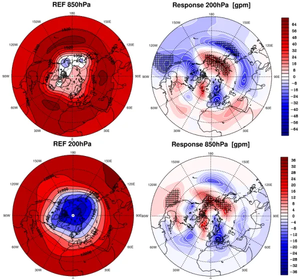
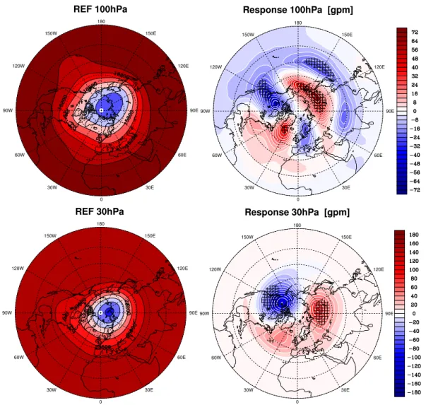
Furthermore looking at geopotential height anomalies November again is highlighted as the only month where a statistically significant response can be found through every level of the atmosphere. For instance the tropospheric low pressure system located at the Aleutian islands (Fig. 8) is sig-nificantly weakened. Looking at stratospheric levels (Fig. 9) the wave number 1 pattern dominates the geopotential re-sponse pattern. In this case this is associated with a shift of the polar vortex center from Asia to the middle of the Arc-tic carrying out a dynamical stabilisation of the polar vor-tex. Consistent to this, the stationary component ofv′T′and
stratospheric temperatures decrease.
In general the stationary component of the meridional heat flux dominates the anomaly pattern of totalv′T′(see Fig. 5).
From January on, the influence of the transient component of v′T′ anomalies are getting stronger, associated with
(a) SW (b) LW
Fig. 7.Outgoing radiation from surface.(a)Respective short-wave (SW) radiation averaged over Arctic region;(b)respective long-wave (LW) radiation averaged over Arctic region. Coloured area covers the 1σ-standard deviation. Black curves indicate absolute difference of REF and NO-ICE.
Fig. 9.Polar stereographic projections of REF simulation stratospheric geopotential at 100 and 30 hPa (left column) in November, and respective response NO-ICE minus REF (right column); colour bar refers only to response pattern. Shaded areas are significant at a 95 % level following student t-test.
transient v′T′ in the NO-ICE simulation attracts the
atten-tion. This decrease counteracts the increase of the stationary component and leads to an insignificant response of the total v′T′. Nevertheless the temporal evolution of the meridional
heat flux anomalies turns out to be largely consistent with the equally non-significant temperature response in the Arc-tic stratosphere (see previous Fig. 2). For instance the overall weakening ofv′T′ in NO-ICE during February is followed
by cooling of Arctic stratospheric temperature in the lead-up of February to March and March itself. This is in agreement with Newman et al. (2001) stating the impact of planetary wave activity on arctic vortex temperature anomalies.
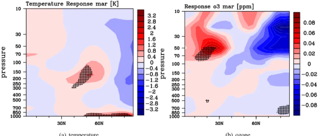
The derived cooling in March is an interesting feature which was also presented in the study of Scinocca et al. (2009). In response to an abrupt sea-ice loss they found for the March mean a strong cooling of the polar atmosphere and a reduction of ozone mixing ratios in this region (see their
Fig. 2). Respective analyses of the E39CA data reveal re-sembling change patterns (Fig. 10). Even though the results shown here are not statistically significant at a 95 % level, we find a high degree of similarity to the results shown by Scinocca et al. (2009). Moreover the statement of Scinocca et al. (2009) that their stratospheric response is mainly dy-namically driven is supported in our study. In particular changes in planetary wave activity in NO-ICE during Febru-ary are related to corresponding Arctic temperature in late February to March.
(a) temperature (b) ozone
Fig. 10.Response NO-ICE minus REF of March mean for.(a)Temperature and(b) ozone. Shaded areas are significant at a 95 % level following student t-test.
(a) Nov–Mar (b) Nov
Fig. 11.Frequency distribution of AO indices for(a)November–March;(b)November seperately. Solid and shaded lines are the running average of two adjacent bins. According to a chi-square test the distribution of NO-ICE differs significantly from REF at a 99 % level.
i.e. a pronounced cooling in the Arctic stratosphere due to a weakened Aleutian Low.
3.5 Leading pattern of Northern Hemisphere AO
As already mentioned in the introduction the stratosphere is intimately connected to the leading variability pattern of at-mospheric circulation also known as the Arctic Oscillation (AO).
For further analyses we computed the AO-index as the daily principal component timeseries of the leading empir-ical orthogonal function of the 1000 hPa geopotential height anomalies (following the calculation procedure as given in Baldwin and Dunkerton, 2001).
Figure 11a displays the frequency distribution of daily AO-indices for the months from November to March for both simulation runs. In comparison to REF the NO-ICE simula-tion shows a growing number of AO in near neutral phase and
at the same time, occurences of high and low AO values tend to decrease. This response is statistically robust. According to a chi square test the distribution of the sensitivity experi-ment deviates significantly at a 99 % level.
This shift to a more neutral state of the AO during winter months can be related to recent studies. They determined a change from strong positive AO trends (in the period of late 1980s to early 1990s) to more neutral AO events (in the late 1990s and early 2000s) although sea ice cover still dramat-ically extenuate (e.g. Overland and Wang, 2005; Maslanik et al., 2007; Zhang et al., 2008).
November obtains a prominent change (according to a chi-square test significant at a 99 % level) to more positive values which correspond to more stable stratospheric condition and a stronger polar vortex (see Fig. 11b).
Often AO is associated with Arctic climate change. As al-ready mentioned in the introduction trends of Arctic surface climate indicators like SAT or SIC are congruent with the variability of the AO. But in the last decade the winter mean of AO-indices tend to be more neutral in difference to the almost linear trends of Arctic climate fields.
Hence suggestions appeared that the Arctic has passed a tipping point into a new climatic state and AO has less in-fluence on Arctic climate (e.g. Lindsay and Zhang, 2005; Maslanik et al., 2007; Zhang et al., 2008). On the other hand Arctic stratospheric temperature during winter, serving as an indicator for the strength of the polar vortex, also shows an episodic character congruent to the AO-index (Overland and Wang, 2005).
3.6 Discussion
The definition of sea-ice perturbation and the corresponding specification of transitions to unperturbed regions must be critically considered in the assessment of sensitivity experi-ments (in this case the NO-ICE simulation).
When comparing the results of different investigations re-garding atmospheric consequences in response to significant Arctic sea-ice reduction it is obvious that the tropospheric re-sponse to sea-ice anomalies is strongly dependent on season and varies regionally. For example there is no clear shifting of the AO-index to positive respective negative values (see ref-erences and discussion in Sect. 3.5 or Sect. 3.1). Nevertheless the overall magnitude of tropospheric changes (e.g. SAT, LW outgoing radiation) due to SIC anomalies are comparable in most of these studies. This gives us confidence that the set-up of the NO-ICE simulation provides a solid basement for estimates of a possible stratospheric responses to a dramatic Arctic sea-ice decrease expected in the future.
Interestingly our findings are in reasonable agreement with the results presented by Orsolini et al. (2012) who used a cou-pled ocean-atmosphere seasonal forced model. In response to the strong Arctic sea-ice reduction on late summer 2007, they found significant warming of the Arctic lower troposphere in the autumn months (regionally up to 10 K near the
sur-emphasised, however, that seasonal and spatial distribution of SST/SIC anomalies varies in all of the studies. Moreover as stated by Orsolini et al. (2012) seasonality could also play a role and this should also be considered in the interpreta-tion of results. Further investigainterpreta-tions of respective long-term data sets, either from observations or numerical studies are needed to confirm this strengthening of the polar vortex in early winter as robust feature.
4 Summary and conclusions
The primary goal of this study was to assess possible conse-quences of a dramatic sea-ice loss during Arctic summer and fall towards stratospheric conditions in all seasons. It was demonstrated that the used model system and the adopted SST/SIC perturbations represent reasonable tropospheric re-sponse which are mostly in line with respective studies pub-lished in literature (e.g. Deser et al., 2004; Alexander et al., 2004; Singarayer et al., 2006; Francis et al., 2009; Budikova, 2009; Screen et al., 2012; Orsolini et al., 2012).
In the current study, the atmospheric background condi-tions are set fixed to the climatology around the year 2000. The derived response to lower and middle stratosphere of a pronounced Arctic sea-ice loss is comparatively weak over the whole year.
During summer small but statistically significant strato-spheric cooling and associated changes in ozone concentra-tion arises which can attributed to radiaconcentra-tion effects due to major changes in the surface albedo.
In the extended winter period (November to March) a sta-tistically robust response is mainly found in November; the detected stratospheric cooling is in rough agreement to find-ings presented by Orsolini et al. (2012) estimating the atmo-spheric reaction on the prominent Arctic sea-ice reduction in the year 2007.
Due to high inter-annual variability of the northern hemi-spheric stratosphere, changes between mid winter and early spring (January to March) are in an overall picture not sta-tistically significant. Nevertheless the detected response in March agrees well with the results of Scinocca et al. (2009) who investigates the effects of an abrupt Arctic sea-ice loss on the ozone layer recovery.
The similarity of our results with those by Orsolini et al. (2012) and Scinocca et al. (2009), although chosen model systems as well as SST/SIC perturbations differ, indicates some robustness in the stratospheric response pattern caused by Arctic sea-ice reduction.
Since this study is only one representation of one specific realisation of investigating sea-ice anomalies further effort are required to gain more general conclusions. The feed-back of melting sea-ice on the ocean circulation, which in turn affects atmospheric circulation (Aagaard and Carmack, 1989; Qiu and Jin, 1997) is not taken into account here, since this study focuses on the mechanism of how changes in SIC affect the stratosphere. Studies that aim to project future stratospheric changes, however need to consider the potential oceanic feedback for reliable results.
Acknowledgements. This study was funded by the Deutsche Forschungsgemeinschaft (DFG) throug the DFG-research group SHARP (stratospheric change and its role for climate prediction) under grant DA 233/3-1. We also want to thank Andreas D¨ornbrack for helpful comments on the manuscript. Futhermore we want to thank two anonymous reviewer for their comments, which improved the quality of the manuscript.
The service charges for this open access publication have been covered by a Research Centre of the Helmholtz Association.
Edited by: M. Van Roozendael
References
Aagaard, K. and Carmack, E. C.: The role of sea ice and other fresh water in the Arctic circulation, J. Geophys. Res., 94, 14485– 14498, doi:10.1029/JC094iC10p14485, 1989.
Alexander, M., Bhatt, U., Walsh, J., Timlin, M., Miller, J., and Scott, J.: The atmospheric response to realistic Artic sea ice anomalies in an AGCM during winter, J. Climate, 17, 890–905, 2004.
Baldwin, M. and Dunkerton, T.:Stratospheric harbingers of anoma-lous weather regimes, Science, 244, 581–584, 2001.
Baldwin, M. and Dunkerton, T.: The solar cycle and stratosphere-troposphere dynamical coupling, J. Atmos. Sol.-Terr. Phy., 67, 71–82, doi:10.1016/j.jastp.2004.07.018, 2005.
Black, R. X.: Stratospheric forcing of surface climate in the Arctic Oscillation, J. Climate, 15, 268–277, 2002.
Budikova, D.: Role of Arctic sea ice in global atmospheric circula-tion: a review, Global Planet. Change, 68, 149–163, 2009. Butler, A. H., Thompson, D. W. J., and Heikes, R.:The
Steady-State Atmospheric Circulation Response to Climate Change-Like Thermal Forcings in a Simple General Circulation Model, J. Climate, 23, 3474–3496, 2010.
Dameris, M.: Climate change and atmospheric chemistry: How will the stratospheric ozone layer develop?, Angew. Chem. Int. Edit., 49, 8092–8102, doi:10.1002/anie.201001643, 2010.
Deser, C. and Teng, H.: Recent trends in Arctic sea ice and the evolving role of atmospheric circulation forcing, 1979–2007. in: Arctic Sea Ice Decline: Observations, Projections, Mecha-nisms, and Implications, Geophysical Monograph 180, edited by: DeWeaver, E. T., Bitz, C. M., and Tremblay, L. B., AGU, 7–26, 2008.
Deser, C., Magnusdottir, G., Saravanan, R., and Phillips, A.: The effects of North Atlantic SST and sea ice anomalies on the winter circulation in CCM3, Part II: Direct and indirect components of the response, J. Climate, 17, 877–889, 2004.
Deser, C., Thomas, R., Alexander, M., and Lawerence, D.: The sea-sonal atmospheric response to projected Arctic Sea ice loss in the late twenty-first-century, J. Climate, 23, 333–351, 2010. Francis, J. A., Chan, W., Leathers, D. L., Miller, J. R., and
Veron, D. E.: Winter Northern Hemisphere weather patterns re-member summer Arctic sea-ice extent, Geophys. Res. Lett., 36, L07503, doi:10.1029/2009GL037274, 2009.
phys. Res., 115D, D00M08, doi:10.1029/2009JD013638, 2010. Haigh, J. D. and Pyle, J. A.: Ozone perturbation experiments in a
two-dimensional circulation model, Q. J. Roy. Meteorol. Soc., 108, 551–574, 1982.
Hegglin, M. I., Gettelman, A., Hoor, P., Krichevsky, R., Man-ney, L. G., Pan, L. L., Son, S.-W., Stiller, G., Tilmes, S., Walker, K. A., Eyring, V., Shepherd, S., Waugh, D., Akiyoshi, H., Anel, J. A., Austin, J., Baumgaertner, A., Bekki, S., Braesicke, P., Br¨uhl, C., Butchart, N., Chipperfield, M., Dameris, M., Dhomse, S., Frith, S., Garny, H., Hardiman, S. C., J¨ockel, P., Kinnison, E. D., Lamarque, J. F., Mancini, E., Michou, M., Mor-genstern, O., Nakamura, T., Olivi, D., Pawson, S., Pitari, G., Plummer, D. A., Pyle, J. A., Rozanov, E., Scinocca, J. F., Shi-bata, K., Smale, D., Teyssdre, H., Tian, W., and Yamashita, Y.: Multimodel assessment of the upper troposphere and lower stratosphere: extratropics, J. Geophys. Res., 115D, D00M09, doi:10.1029/2010JD013884, 2010.
Holland, M. M., Bitz, C. M., and Tremblay, B.: Future abrupt re-ductions in the summer Artic sea ice, Geophys. Res. Lett., 33, L23503, doi:10.1029/2006GL028024, 2006.
Holland, M. M., Bitz, C. M., Tremblay, B., and Bailey, D. A.: The role of natural versus forced change in future rapid summer Arc-tic ice loss, in: ArcArc-tic Sea Ice Decline: Observations, Projections, Mechanisms, and Implications, Geophysical Monograph 180, edited by: DeWeaver, E. T., Bitz, C. M., and Tremblay, L. B., AGU, 133–150, 2008.
Hurrell, J. W. and Deser, C.: North Atlantic climate variability: the role of the North Atlantic oscillation, J. Mar. Syst., 78, 28–41, doi:10.1016/j.jmarsys.2008.11.026, 2009.
IPCC: Climate Change 2001 – The physical science basis, Tech. rep., Intergovernmental Panel on Climate Change, Cam-bridge University Press, New York, USA, 2001.
IPCC: Climate Change 2007 – The physical science basis, Tech. rep., Intergovernmental Panel on Climate Change, Cam-bridge University Press, New York, USA, 2007.
Johns, T. C., Durman, C. F., Banks, H. T., Roberts, M. J., McLaren, A. J., Ridley, J. K., Senior, C. A., Williams, K. D., Jones, A., Rickard, G. J., Cusack, S., Ingram, W. J., Cruci-fix, M., Sexton, D. M. H., Joshi, M. M., Dong, B., Spencer, H., Hill, R. S. R., Gregory, J. M., Keen, A. B., Pardaens, A. K., Lowe, J. A., Bodas-Salcedo, A., Stark, S., and Searl, Y.: The new Hadley Centre Climate Model (HadGEM1): evaluation of coupled simulations, J. Climate, 19, 1327–1353, 2006.
Kumar, A., Perlwitz, J., Eischeid, J., Quan, X., Xu, T., Zhang, T., Hoerling, M., Jha, B., and Wang, W.: Contribution of sea ice loss to Arctic amplification, Geophys. Res. Lett., 37, L21701, doi:10.1029/2010GL045022, 2010.
sphere in the new Hadley Centre Global Environmental Model (HadGEM1), Part 1: Model description and global climatology, J. Climate, 19, 1274–1301, 2006.
Maslanik, J., Drobot, S., Fowler, C., Emery, W., and Barry, R.: On the Arctic climate paradox and the continuing role of atmo-spheric circulation in affecting sea ice conditions, Geophys. Res. Lett., 34, L03711, doi:10.1029/2006GL028269, 2007.
Newman, P., Nash, E., and Rosenfield, J.: What controls the temper-ature of the Artic stratosphere during spring?, J. Geophys. Res., 106, 19999–20010, 2001.
Orsolini, Y., Senan, R., Benestad, R. E., and Melsom, A.: Autumn atmospheric response to the 2007 low Arctic sea ice extent in coupled ocean-atmosphere hindcasts, Clim. Dynam., 38, 2437– 2448, 2012.
Overland, J. E. and Wang, M.: Arctic climate paradox: the recent de-crease of the Arctic oscillation, Geophys. Res. Lett., 32, L06701, doi:10.1029/2004GL021752, 2005.
Overland, J. E. and Wang, M.: Large-scale atmospheric circulation changes are associated with the recent loss of Arctic sea ice, Tel-lus A, 62, 1–9, doi:10.1111/j.1600-0870.2009.00421.x, 2010. Overland, J. E., Wang, M., and Salo, S.: The recent Arctic warm
period, Tellus A, 60, 589–597.
Parkinson, C., Rind, D., Healy, R., and Martinson, D.: The impact of sea ice concentration accuracies on climate model simulations with the GISS GCM, J. Climate, 14, 2606–2623, 2001. Qiu, B. and Jin, F. F.: Antarctic circumpolar waves: an indication
of ocean-atmosphere coupling in the extratropics, Geophys. Res. Lett., 20, 2585–2588, doi:10.1029/JC094iC10p14485, 1997. Reithmeier, C. and Sausen, R.: ATTILA: Atmospheric tracer
trans-port in a Lagrangian model, Tellus B, 54, 278–299, 2002. Rind, D., Perlwitz, J., and Lonergan, P.: AO/NAO response to
climate change: 1. Respective influences of stratospheric and tropospheric climate changes, J. Geophys. Res., 110, D12107, doi:10.1029/2004JD005103, 2005.
Scaife, A. A., Knight, J. R., Vallis, G. K., and Folland, C. K.: A stratospheric influence on the winter NAO and North Atlantic surface climate, Geophys. Res. Lett., 32, L18715, doi:10.1029/2005GL023226, 2005.
Schnadt, C. and Dameris, M.: Relationship between North At-lantic Oscillation changes and stratospheric ozone recovery in the Northern Hemisphere in a chemistry-climate model, J. Geo-phys. Res., 30, 1487, doi:10.1029/2003GL017006, 2003. Scinocca, J. F., Reader, M., Plummer, P., Sigmond, M., Kushner, P.,
Screen, J. A., Deser, C., and Simmonds, I.:Local and remote controls on observed Artic warming, Geophys. Res. Lett., 39, L10709, doi:10.1029/2012GL051598, 2012.
Seierstad, I. and Bader, J.: Impact of a projected future Artic sea ice reduction on extratropical storminess and the NAO, Clim. Dy-nam., 33, 937–943, 2009.
Serreze, M. C., Barrett, A. P., Stroeve, J. C., Kindig, D. N., and Hol-land, M. M.: The emergence of surface-based Arctic amplifica-tion, The Cryosphere, 3, 11–19, doi:10.5194/tc-3-11-2009, 2009. Singarayer, J., Bamber, J., and Valdes, P.: Twenty-first-century cli-mate impacts from a declining Arctic sea ice cover, J. Clicli-mate, 19, 1109–1125, 2006.
SPARC CCM Val: Eyring, V., Shepherd, T., and Waugh, D. E.: SPARC CCMVal Report on the Evaluation of Chemistry-Climate Models, Tech. rep., SPARC Report No. 5, WCRP-132, WMO/TD-No. 1526, 2010.
Steil, B., Dameris, M., Br¨uhl, C., Crutzen, P. J., Grewe, V., Ponater, M., and Sausen, R.: Development of a chemistry module for GCMs: first results of a multiannual integration, Ann. Geophys., 16, 205–228, doi:10.1007/s00585-998-0205-8, 1998.
Stenke, A., Grewe, V., and Ponater, M.: Lagrangian transport of wa-ter vapor and cloud wawa-ter in the ECHAM4 GCM and its impact on the cold bias, Clim. Dynam., 31, 491–506, 2008.
Stenke, A., Dameris, M., Grewe, V., and Garny, H.: Implica-tions of Lagrangian transport for simulaImplica-tions with a coupled chemistry-climate model, Atmos. Chem. Phys., 9, 5489–5504, doi:10.5194/acp-9-5489-2009, 2009.
Stroeve, J., Holland, M., Meier, W., Scambos, T., and Serreze, M.: Artic sea ice decline: faster than forecast, Geophys. Res. Lett., 34, L09501, doi:10.1029/2007GL029703, 2007.
Thompson, D. W. J. and Wallace, J. M.: The Arctic oscillation signature in the wintertime geopotential height and temperature fields, Geophys. Res. Lett., 25, 1297–1300, 1998.
Thompson, D. W. J., Wallace, J. M., and Hegerl, G. C.: Annular modes in the extratropical circulation, Part II: Trends, J. Climate, 13, 1018–1036, 2000.
Wang, J. and Ikeda, M.: Arctic oscillation and Arctic sea-ice oscil-lation, Geophys. Res. Lett., 27, 1287–1290, 2000.
WMO (World Meteorological Organization):Scientific Assessment of Ozone Depletion: 2006, Global Ozone Research and Monitor-ing Project-Report No. 50, 572 pp., Geneva, Switzerland, 2007. WMO (World Meteorological Organization):Scientific Assessment
of Ozone Depletion: 2010, Global Ozone Research and Monitor-ing Project-Report No. 52, 516 pp., Geneva, Switzerland, 2011. Wu, B., Wang, J., and Walsh, J. E.: Dipole anomaly in the winter
Arctic atmosphere and its association with sea ice motion, J. Cli-mate, 19, 210–225, 2006.