Use of laboratory and remote sensing techniques to estimate vegetation patch scale emissions of nitric oxide from an arid Kalahari savanna

(1)

BGD

5, 4621–4680, 2008

Nitric oxide emissions from an arid Kalahari savanna

G. T. Feig et al.

Title Page

Abstract Introduction

Conclusions References

Tables Figures

◭ ◮

Back Close

Full Screen / Esc

Printer-friendly Version

Interactive Discussion

Biogeosciences Discuss., 5, 4621–4680, 2008 www.biogeosciences-discuss.net/5/4621/2008/ © Author(s) 2008. This work is distributed under the Creative Commons Attribution 3.0 License.

Biogeosciences Discussions

Biogeosciences Discussionsis the access reviewed discussion forum ofBiogeosciences

Use of laboratory and remote sensing

techniques to estimate vegetation patch

scale emissions of nitric oxide from an

arid Kalahari savanna

G. T. Feig1, B. Mamtimin2, and F. X. Meixner3

1

Max Planck Institute for Chemistry, Biogeochemistry Department P.O. Box 3060, 55020 Mainz, Germany

2

Department of Physics University of Zimbabwe, Harare, Zimbabwe

3

Institute of Geography Science and Tourism, Xinjiang Normal University, P.R. China

Received: 15 September 2008 – Accepted: 6 October 2008 – Published: 3 December 2008 Correspondence to: G. Feig (feig@mpch-mainz.mpg.de)

(2)

BGD

5, 4621–4680, 2008

G. T. Feig et al.

Title Page

Tables Figures

◭ ◮

Back Close

Full Screen / Esc

Abstract

The biogenic emission of nitric oxide (NO) from the soil has an important impact on a number of environmental issues, such as the production of tropospheric ozone, the cy-cle of the hydroxyl radical (OH) and the production of NO. In this study we collected soils from four diff_{ering vegetation patch types (Pan, Annual Grassland, Perennial Grassland} 5

and Bush Encroached) in an arid savanna ecosystem in the Kalahari (Botswana). A laboratory incubation technique was used to determine the net potential NO flux from the soils as a function of the soil moisture and the soil temperature. The net potential NO emissions were up-scaled for the year 2006 and a region (185 km×185 km) of the

southern Kalahari. For that we used (a) the net potential NO emissions measured in

10

the laboratory, (b) the vegetation patch distribution obtained from Landsat NDVI surements, (c) estimated soil moisture contents obtained from ENVISAT ASAR mea-surements and (d) the soil surface temperature estimated using MODIS MOD11A2 8 day land surface temperature measurements. Diff_{erences in the net potential NO}

fluxes between vegetation patches occur and range from 0.27 ng m−2s−1 in the Pan

15

patches to 2.95 ng m−2s−1in the Perennial Grassland patches. Up-scaling the net po-tential NO fluxes with the satellite derived soil moisture and temperature data gave NO fluxes of up to 323 g ha−1month−1, where the highest up-scaled NO fluxes occurred in the Perennial Grassland patches, and the lowest in the Pan patches. A marked sea-sonal pattern was observed where the highest fluxes occurred in the austral summer

20

months (January and February) while the minimum fluxes occurred in the austral win-ter months (June and July), and were less than 1.8 g ha−1month−1. Over the course of the year the mean NO emission for the up-scaled region was 0.54 kg ha−1_yr−1_{, which}

accounts for a loss of up to 7.4% of the nitrogen (N) input to the region through atmo-spheric deposition and biological N fixation. The biogenic emission of NO from the soil

25

(3)

BGD

5, 4621–4680, 2008

G. T. Feig et al.

Title Page

Tables Figures

◭ ◮

Back Close

Full Screen / Esc

1 Introduction

The concentrations of nitric oxide (NO) and nitrogen dioxide (NO2) (collectively known

as NOx) are important in regulating chemical reactions of the atmosphere (Crutzen,

1995; Crutzen and Lelieveld, 2001; Monks, 2005). They control the production and de-struction of tropospheric ozone (Chameides et al., 1992; Crutzen and Lelieveld, 2001),

5

are involved in the cycle of the OH radical (the most important tropospheric cleansing agent) and in the production of nitric acid (HNO₃) (Logan, 1983; Meixner, 1994; Monks, 2005; Steinkamp et al., 2008). The global emissions of NOx have been severely

al-tered by anthropogenic activity. In 1860 global NOx emissions were estimated to be

13 Tg yr−1of which the majority is thought to have come from natural sources such as

10

soils and lightning (Galloway et al., 2004). The recent estimate of the IPCC puts total NOx emissions at 42–47 Tg yr−

1

with the most important source being fossil fuel com-bustion (Denman et al., 2007), and soil is thought to account for between 10% to 40% of the total NO emissions (Davidson and Kingerlee, 1997; Denman et al., 2007). Over 40% of the total NO emissions from Africa are supposed to originate from biogenic

pro-15

duction in the soil (Jaegle et al., 2004). The wide range of uncertainty is partly due to insuffi_{cient measurements, particularly in the drylands (Galbally et al., 2008). A recent}

review by Meixner and Yang (2006) only identified 13 studies in natural ecosystems receiving less than 400 mm rain a year (since then three other studies have occurred (Feig et al., 2008; Holst et al., 2007; McCalley and Sparks, 2008), this is problematic

20

since drylands make up a sizable proportion of the earth’s surface area and are thought to be capable of substantial emissions of NO (Davidson and Kingerlee, 1997).

The biogenic production of NO in the drylands is dominated by the process of nitrifi-cation (Conrad, 1996; Galbally et al., 2008). Nitrifinitrifi-cation is influenced by environmental factors, such as the soil moisture, the soil temperature and the soil nutrient content.

25

(4)

BGD

5, 4621–4680, 2008

G. T. Feig et al.

Title Page

Tables Figures

◭ ◮

Back Close

Full Screen / Esc

In drier ecosystems, soil water seems to be the most important factor regulating emis-sions of NO. When the soil moisture is too low to maintain microbial activity there are very low levels of NO emitted (Galbally et al., 2008; Garrido et al., 2002; Meixner et al., 1997) and when soil moisture levels are too high to maintain aerobic conditions, the emission of NO is negligible (Skopp et al., 1990). The optimal emission of NO in

5

drylands seems to occur at low soil moisture levels, but where microbial activity can still take place. In a previous laboratory based study in the Kalahari, NO emissions were very low at both high and low soil moisture contents, while the optimum soil moisture for NO production was approximately 20% Water Filled Pore Space (WFPS) (Aranibar et al., 2004). Since the biogenic production of NO is mostly a bacterially mediated

10

process, temperature has an important impact on the rate of the reaction, and as the environmental temperature increases so does the rate of nitrification and hence the release of NO. A number of previous studies have shown that the rate of NO increase approximately doubles with a 10◦_{C increase in temperature (Feig et al., 2008; Kirkman}

et al., 2001; McCalley and Sparks, 2008). The soil nutrient status is another important

15

controller of biogenic NO emissions; many studies have found a relationship between the emissions of NO and either the concentrations of ammonia or nitrate (Erickson et al., 2002, 2001; Hartley and Schlesinger, 2000; Hutchinson et al., 1993; Ludwig et al., 2001; Meixner et al., 1997; Parsons et al., 1996) or the N cycling rate (Erickson et al., 2002, 2001; Hartley and Schlesinger, 2000; Parsons et al., 1996). Therefore, natural

20

or anthropogenic actions that result in the modification of the inputs of nutrients or the rates of nutrient turnover are likely to have an eff_{ect on the NO production rates.}

The Kalahari ecosystem extends from South Africa, through Botswana and into Zam-bia and covers an area of 2.5 million km2, it is an ecosystem occurring on a homoge-nous substrate. A rainfall gradient exists, from approximately 200 mm yr−1in the south

25

to over 1000 mm yr−1 _{in the north, this results in a gradient of vegetation, from sparse}

(5)

BGD

5, 4621–4680, 2008

G. T. Feig et al.

Title Page

Tables Figures

◭ ◮

Back Close

Full Screen / Esc

The Kalahari is currently undergoing extensive land use change associated with an increase in pastoral land use, which has been made possible with the introduction of boreholes to provide water for livestock. Grazing is concentrated around the perma-nent water sources and creates a distinctive disturbance pattern of concentric vegeta-tion zones. Typically in the close vicinity to the water source there is what has been

5

termed the “sacrifice zone” where there is heavy disturbance; this is followed by a “bush encroached” where there is a strong increase in the proportion of woody shrub veg-etation, typically dominated by (Acacia mellifera) (Dougill and Thomas, 2004; Hagos and Smit, 2005; Thomas and Dougill, 2007) resulting from the preferential use of grass species by cattle. Beyond the bush encroached zone, where there is less disturbance,

10

the later successional stages of vegetation occur.

The vegetation is known to have an eff_{ect on the quantity and cycling of nutrients}

(Hagos and Smit, 2005). This has been shown to influence the emission of NO from the soil, for example in Texas the emission of NO is higher under areas where there has been encroachment ofProsopis sp. (Hartley and Schlesinger, 2000; Martin and

15

Asner, 2005; Martin et al., 2003a). These previous studies have either looked at the larger landscape scale (Aranibar et al., 2004; Br ¨ummer et al., 2008; Davidson, 1991a; Delon et al., 2007; Hartley and Schlesinger, 2000; Jaegle et al., 2004; Martin et al., 2003b; Otter et al., 1999; Serca et al., 1998) or at the vegetation canopy scale (Barger et al., 2005; Hall and Asner, 2007; Hartley and Schlesinger, 2000; Holst et al., 2007;

20

Le Roux and Abbadie, 1995; Levine et al., 1996; Martin et al., 1998; McCalley and Sparks, 2008; Meixner et al., 1997; Mosier et al., 2003; Smart et al., 1999); however there is a need to determine what occurs in the emission of NO between the plant canopy scale and the vegetation patch scale which has been examined in only very few studies (Kirkman et al., 2001; Martin and Asner, 2005; Scholes et al., 1997; Van

25

Dijk et al., 2002). The main points of consideration in this study are (1) to determine the eff_{ect of di}ff_{ering vegetation cover types on the emission of NO along a disturbance}

(6)

BGD

5, 4621–4680, 2008

G. T. Feig et al.

Title Page

Tables Figures

◭ ◮

Back Close

Full Screen / Esc

2 Methods and materials

2.1 Site

The site of the research was at the Berry Bush Farm (25◦₅₆′_{47.73 S, 22}◦₂₅′_{39.47 E,}

elevation 978 m), a 900 ha commercial ranch, situated approximately 10 km north east of the town of Tsabong in the Kgalagadi District, Botswana. The ranch was formerly

5

used for cattle and sheep farming but at the time of sampling, in May 2006, the stock densities had been reduced and it was only grazed by approximately 120 springbok and other small game. The area has been described as a grass bush savanna (Dougill and Thomas, 2004) and is situated on the southern portion of the Kalahari sands. The soils in the Kalahari sands are typically deficient in nutrients, deep, structureless and

10

consist of an average of 62% fine quartz sand in all horizons (Ringrose et al., 1998). The Kalahari is in a highly seasonal (austral) summer rainfall region, with very high inter-annual variability (Thomas and Dougill, 2007). Mean rainfall measured at the offi_{cial meteorological station at Berry Bush Farm is 280 mm yr}−1 _{with a 32% annual}

variability for the period 1997–2005 (Keith Thomas, personal communication). At the

15

Tsabong WMO station (WMO Index number 68328) it has been reported that it has a mean annual rainfall of approximately 300 mm with a 45% inter-annual variability (Thomas and Dougill, 2007). The year of sampling, 2006, was a very wet year and 418 mm of rain had fallen by the time the soil samples were taken in May.

Four main types of vegetation patches occur on the Berry Bush Farm and are thought

20

to represent a repeated vegetation pattern for the region. The four vegetation patches are; Annual Grassland, Perennial Grassland, bush Encroachment and Pan. From the four main types of vegetation patches that occur on the Berry Bush Farm three of the patches, namely; Perennial Grassland, Annual Grassland and Encroachment corre-spond to diff_{ering successional stages in the disturbance regime (where the Perennial} 25

(7)

BGD

5, 4621–4680, 2008

G. T. Feig et al.

Title Page

Tables Figures

◭ ◮

Back Close

Full Screen / Esc

2.2 Soil and vegetation sampling

Three replicate sampling sites were selected in each of the vegetation patch types. At each of the sampling sites three 25 m transects were laid out at 120◦ _{to each other.}

The plant cover was estimated as the vegetation cover directly over the transect line and was assigned to various vegetation structural classes, if more than one structural

5

unit overlapped, the larger more physically dominant was recorded. Six diff_erent

veg-etation structural classes have been defined which consisted of; perennial grasses, annual grasses (grasses were classified as annual or perennial species according to Van Oudtshorn (1999)), tree cover, soil crusts, bare soil and other (including shrubs and forbs). For each of the vegetation patch types the total aerial cover was estimated

10

from the sum of the nine transects (three replicates of each vegetation patch and three 25 m transects within each replicate).

In each of the sampling sites ten soil samples (approx. 150 g) were taken under each of three vegetation types; tree cover, grass cover and open, these were then combined to make a representative soil sample of approximately 1.5 kg in mass (four vegetation

15

patches, three replicates of each vegetation patch, and three vegetation types giving a total of thirty nine 1.5 kg soil samples). In the Pan ten soil sub-samples were also taken under soil crust. The soil crusts were defined according to the classification of Dougill and Thomas (2004), however only the second and third stage crusts were sampled, since these were the most developed and were clearly discernable. The soil

20

was air dried, sieved through 2 mm mesh and stored at 5◦C until use. Within each of the vegetation types the soil bulk density was measured in the first 5 cm using a stainless steel soil core of known volume.

The soil texture was determined using a hydrometer technique after the method of (Day, 1969) and the soil pH was measured in 2.5:1 mixture in distilled water according

25

(8)

BGD

5, 4621–4680, 2008

G. T. Feig et al.

Title Page

Tables Figures

◭ ◮

Back Close

Full Screen / Esc

set up to measure total C, and N contents of the soil.

2.3 Laboratory incubation and net NO release from soil

Two days before beginning the measurements, the soil was soaked with deionised water and allowed to drain freely at room temperature (22◦C), this was to limit the con-founding eff_{ect of pulsing after the initial wetting of soil after a long period of inactivity.} 5

Pulsing is known to elicit a large but temporally limited emission. The magnitude of the pulse after rewetting the soil is variable depending on the preceding period of time in which the soil was dry. Since this can not be easily controlled and pulsing is thought to add a fairly minor contribution to the annual NO flux, reported to be less than 6% (Scholes et al., 1997) we decided to neglect the eff_{ect of pulsing in this study, which} 10

means that the fluxes that are calculated here should be considered to be a lower limit. The basic methodology for the laboratory measurement of the NO flux from soil has been previously described (Aranibar et al., 2004; Kirkman et al., 2001; Meixner and Yang, 2006; Otter et al., 1999; Van Dijk et al., 2002) and was further developed by Feig et al. (2008). It has been shown that there is good agreement between

labora-15

tory fluxes of NO calculated according to this method and the measured field fluxes (Ludwig et al., 2001; Meixner et al., 1997; Van Dijk et al., 2002). Briefly; a known quantity (approximately 100 g (dry weight)) of sieved, wetted soil was placed in one of five plexiglas chambers (volume 0.97 l) in a thermo-controlled cabinet. Pressurised air that had passed through a purification system was supplied to each chamber at a

20

flow rate of 4.2×10−5m3s−1(2.5 L min−1). The outlet of each chamber was connected

via a reversed Naphion drier (series MD-110, Perma Pure LLC, USA) and a switching valve to a NO Chemoluminescence analyser (CLD780TR, Eco Physics Switzerland) and a H₂O/CO₂ analyser (Binos IR gas analyser, Rosemont Analytical, USA). Nitric oxide standard gas (200 ppm) was attached to the air purification system via a mass

25

(9)

BGD

5, 4621–4680, 2008

G. T. Feig et al.

Title Page

Tables Figures

◭ ◮

Back Close

Full Screen / Esc

was determined by integrating the loss of water vapour throughout the measurement period and relating it to the gravimetric soil moisture content at the start and end of the measurement.

2.4 Measurements of the net NO release rate

The net release of NO (J_NO, in ng kg−1s−1) (all units are in terms of mass of N and dry

5

mass of soil) is calculated from the diff_{erence between the NO mixing ratio at the outlet}

of the reference cuvette and the outlet of each of the incubation cuvettes (since the air in the cuvette is well mixed by a microfan, the air at the outlet is assumed to have the same composition as the air in the headspace) according to:

J_NO= Q

M_soil mNO,out−mNO,ref

×

_M

N

V_m ×10

−3

(1)

10

WhereQis the flow rate through the cuvette (4.2×10−5m3s−1 or 2.5 L min−1),Msoilis

the dry mass of the soil (kg),M_Nis the molar mass of N (14.0076 kg kmol−1_),_V

mis the molar volume (24.465 m3kmol−1

at 25◦_{C, 1013.25 hPa) and} _m

NO,ref and mNO,out are

the mixing ratios of NO in ppb, at the outlets of the reference and incubation cuvettes, respectively. The factorM_N/V_m_×10−3is needed to convert NO mixing ratio (ppb) to NO

15

concentration (ng m−3_).

The release of NO from the soil is the result of the microbial production and con-sumption of NO in the soil, processes that occur simultaneously (Conrad, 1994, 1996; Conrad and Smith, 1995). As a result, the NO release rate (J_NO) is always a net release rate. However if the NO consumption is greater than production in the soil sample then

20

J_NO becomes negative. This will only occur if the in-coming (=_{reference) NO mixing}

ratio is greater than the headspace NO mixing ratio in the soil containing chamber. It has already been shown experimentally that there is a linear relationship between the NO release rate (J_NO) and the rates of NO production (P) and NO consumption (k) (Ludwig et al., 2001; Remde et al., 1989) so that the measured release rates can be

(10)

BGD

5, 4621–4680, 2008

G. T. Feig et al.

Title Page

Tables Figures

◭ ◮

Back Close

Full Screen / Esc

described according to:

J_NO=_P ₋_k_×_m_NO_,_out_×

_M

N

V_m ×10

−3

(2)

This equation implies that the NO production is independent of the NO mixing ratio in the headspace (m_NO_,_out), while the NO consumption is dependent on the NO mixing ratio in the headspace, and can be approached as a first order decay process. To

5

determine the values ofP and k, Eq. (2) was used with the measured release rates (J_NO) from two sets of incubation measurements, namely usingm_NO_,_ref_,_low=_{0 ppb and}

m_NO_,_ref_,_high=_{58 ppb. This allowed us to calculate}_P _{(ng kg}−1_s−1_{) and}_k _(m3_kg−2_s−2_),

wherekcan be determined from the slope of Eq. (2),

k= ∆JNO

∆_[NO]

= JNO,high−JNO,low

m_NO_,_high₋m_NO_,_low ×

_V m

M_N ×10

3

(3)

10

Where m_NO_,_low is the actual NO mixing ratio (ppb) in the head space of the cuvette under fumigation with NO free air and m_NO_,_high is the actual NO mixing ratio in the cuvette headspace under fumigation with 58 ppb NO. In this study, we will present values of the NO release rate (J_NO) as a function of soil moisture, in terms of the soil WFPS. Water filled pore space is a useful concept because it indicates the amount

15

of water in the soil that is available for microbial activity and also the amount of air in the soil (and therefore the soil oxygen status). The WFPS is calculated (a) from the amount of water lost from the enclosed cuvettes through evaporation during the incubation process and (b) through determining the gravimetric water content (Θ_{) of}

the wetted sample at the start of the incubation. The WFPS is calculated according to

20

Eq. (4):

WFPS=Θ_× BD

1−BD_{P D}

(4)

(11)

BGD

5, 4621–4680, 2008

G. T. Feig et al.

Title Page

Tables Figures

◭ ◮

Back Close

Full Screen / Esc

and drying the soil at 105◦_{C for 48 h, and}_PD_{is the particle density of the average soil}

mineral (quartz) with a value of 2.65×103kg m−3according to (Parton et al., 2001).

2.5 Calculation of the net potential NO flux

The laboratory derived net release of NO (J_NO, in ng kg−1s−1) from the soil was con-verted to a net potential NO flux (F_lab, in ng m−2s−1) using a simple diff_{usion based} 5

algorithm (Eq. 5), originally developed by (Galbally and Johansson, 1989), modified by van Dijk et al. (2002). The net potential laboratory NO flux, as a function of WFPS and T_soil, is calculated according to:

Flab(Tsoil,WFPS)=

q

BD×k(Tsoil,WFPS)×D(WFPS)×

_P₍_T

soil,WFPS)

k(Tsoil,WFPS)

−[NO]Headspace (5)

Where [NO]Headspace is the NO concentration (in 10− 12

kg m−3) in the headspace of

10

the cuvette; D(WFPS), in m2s−1, is the WFPS dependent diff_{usion coe}ffi_{cient of NO}

through the soil, calculated after Moldrup et al. (2000), from the WFPS and the gas diff_{usion constant for free air (m}2_s−1_{) equal to 1.9}_×₁₀−5_m−2_s−1 _{(Gut et al., 1998).}

The diff_{usion coe}ffi_{cient is dependent of the soil moisture content and the soil bulk}

density and therefore is calculated for each soil sample and each soil moisture interval.

15

For a given soil temperature, an algorithm has been developed (Meixner and Yang, 2006) to fit our net potential NO fluxes as a function of the WFPS (Eq. 5). This algorithm describes the net potential NO flux as a power increase until optimal soil moisture followed by an exponential decrease:

F_lab(T_soil=_const_.,_WFPS)=_a_WFPSb_exp(₋_c_WFPS) ₍₆₎ 20

Where parametersa,bandcare related to observed values by:

a= Flab(WFPSopt)

h

WFPSb_optexp(−b)

(12)

BGD

5, 4621–4680, 2008

G. T. Feig et al.

Title Page

Tables Figures

◭ ◮

Back Close

Full Screen / Esc

b=

lnh_FFlab(WFPSopt)

lab(WFPSupp)

i

ln_WFPSWFPSopt

upp

+WFPSupp WFPS_opt −1

(8)

c= −b

WFPSopt

(9)

Where, for a given T_soil, WFPSopt is the soil moisture where the maximum

labo-ratory NO release is observed, F_lab(WFPSopt) is the maximum net potential NO flux

at the WFPS_opt (the optimum WFPS), and WFPS_upp is the soil moisture content

5

where F_lab approximately equals zero (i.e. F_lab (WFPSupp)=1/100Flab (WFPSopt) for

WFPS>WFPSopt).

The temperature dependence of the laboratory NO flux was determined by calcu-lating the net potential NO flux at two soil temperatures, 25◦C and at 35◦C. The tem-perature dependence usually shows an exponential increase and can be expressed as

10

the increase ofF_labfor a 10◦_{C increase in soil temperature, otherwise known as a}_Q 10

function (Eq. 10) (Lloyd and Taylor, 1994).

Q₁₀(WFPS)=Flab(Tsoil

=₃₅◦_C_,_WFPS)

F_lab(T_soil=₂₅◦_C_,_WFPS) (10)

The Q₁₀ function can then be included into Eq. (6), as a “temperature amplification factor” of the reference NO flux (T_ref=₂₅◦_{C), so that the laboratory NO flux can be} 15

estimated as a function of both soil temperature and soil moisture (Eq. 11):

F_lab(T_soil,WFPS)=_a

TrefWFPS

bT_ref_exp

−cTref×WFPS

×exp

_ln_Q

10(WFPS)

10 ×(Tsoil−Tref)

(11)

2.6 Compensation point mixing ratio

The compensation point mixing ratio (m_NO_,_comp) is an important concept for the bi-directional exchange of NO (see (Conrad, 1994)). Since it determines what the ambient

(13)

BGD

5, 4621–4680, 2008

G. T. Feig et al.

Title Page

Tables Figures

◭ ◮

Back Close

Full Screen / Esc

mixing ratio of NO in the atmosphere has to be before a net NO uptake into the soil can occur. The compensation point mixing ratio is calculated by resolving Eq. (5) for the NO concentration whereF_lab(WFPS,T_soil)=_0:

m_NO_,_comp(T_soil,WFPS)=P(Tsoil,WFPS)

k(T_soil,WFPS)×

_V

m

M_N ×10

3

(12)

In Eq. (5) the last term considers them_NO_,_compand the ambient NO concentration,

how-5

ever it has to be stated that them_NO_,_comphas been found to be much larger (60–90 ppb, see Sect. 4.4.2) than the ambient NO mixing ratio in the Kalahari region (<0.8 ppb, see Sect. 4.4.1).

2.7 Error estimation of NO release measurements

To determine the detection limit of ourJ release measurements, inert glass beads and

10

autoclaved soils were used to measure the “blank” net release of NO as shown in the study of Feig et al. (2008). It was found that the “blank” net release of NO from the glass beads was at a rate of 0.02 ng kg−1s−1, with a random deviation of 0.02 ng kg−1s−1 ir-respective of the moisture content, therefore an experimentally derived detection limit for J_NO of 0.08 ng kg−1s−1 may be considered. This results from the mean release

15

rate of glass beads plus 3 standard deviations (corresponding to a confidence inter-val of 99.7%). Similarly, the detection limit of the autoclaved soils is 0.11 ng kg−1_s−1_,

therefore the more conservative estimate from the autoclaved soils was used as our detection limit.

To quantify the precision ofJ_NOmeasurements, the NO net release rate was

deter-20

mined experimentally through the simultaneous measurement of four replicates across the full range of soil moisture. The mean standard deviation on the NO net release rate was found to be 0.03 ng kg−1s−1 irrespective of WFPS; this is lower than the experi-mentally derived detection limit ofJ_NO. We consider±0.05 ng kg−1s−1as a

conserva-tive estimate of the experimentally derived precision ofJ_NO.

(14)

BGD

5, 4621–4680, 2008

G. T. Feig et al.

Title Page

Tables Figures

◭ ◮

Back Close

Full Screen / Esc

An error propagation approach was used to estimate the error in the net potential NO flux (Harris, 1995). The error in the net potential NO flux is derived from the error of mixing ratio measurements (i.e., error of the NO analyser), error in the determination of the bulk density, error in the determination of the consumption constantk, error in the calculation of the diff_{usion values and error in the determination of NO production} 5

values (P) (which can be assumed to be similar to those of the J release) and the error in the water vapour measurement which is mainly the WFPS measurements (see Eq. 5).

– The error in the NO_Headspace measurements stems from the sensitivity of the NO analyser; using 37 diff_{erent measurement periods (over 13 000 individual data} 10

points) during January–October 2006 the instrument noise was found to be 0.75% of the corresponding signal.

– The error in the BD calculation was determined from:

– The error in the balance (Model, Sartorius, G ¨ottingen, Germany) this was found to be±0.006 g from 20 sets of measurements in a mass range of 2–

15

1000 g. The error was determined for a mass of 150 g giving a relative error of 0.004%.

– A maximum relative error of 5% was assumed (conservatively) for determi-nation of the volume of the soil sample which was finally used as the error of the BD calculations.

20

– The error in the consumption constant k was calculated using the absolute er-ror calculated forJ (0.04 ng kg−1_s−1_{) and converted to a relative error using a}_J

release value of 3.5 ng kg−1s−1), this and the relative error of the NO analyser (0.75%), resulted in a relative error ink of 1.7%.

– The noise in the water vapour measurements was determined by adding water to

25

(15)

BGD

5, 4621–4680, 2008

G. T. Feig et al.

Title Page

Tables Figures

◭ ◮

Back Close

Full Screen / Esc

– The relative error in the diff_{usion values is derived from a 0.8% relative error in}

the water vapour measurements and a 5% assumed error for the bulk density measurements resulting in a relative error in the diff_{usion values of 5.1%}

– The error in P can be calculated from the errors in J, k and the m_NO_,_headspace and it is found that the absolute error ofP is 0.07 ng kg−1_s−1_{and if a maximum}_P 5

value of 3.5 ng kg−1s−1is assumed, this gives a relative error of 2% inP.

Propagating the errors of all these variables, results in a relative error of 4.2% of the net potential NO flux.

2.8 Statistics and analysis

Calculations and graphs have all been done in EXCEL (Microsoft®), and IGOR®

Ver-10

sion 6.03, while statistical analysis of the soil physical and chemical properties was done using a 2 way ANOVA after checking for normality; all statistics were done using SPSS version 16.

2.9 Up-scaling to the regional level using remote sensing and GIS techniques

The calculated net potential NO flux values (as a function of soil moisture and

temper-15

ature, see Eq. 11) were used to create a regional estimate of the NO flux (F_up₋_scaled) under a GIS framework. To do this, three tools were developed for the use of remote sensing information. These were the following classification schemes of:

– Land use (vegetation patch); – Soil temperature;

20

– Soil moisture.

(16)

BGD

5, 4621–4680, 2008

G. T. Feig et al.

Title Page

Tables Figures

◭ ◮

Back Close

Full Screen / Esc

2.9.1 Land use classification

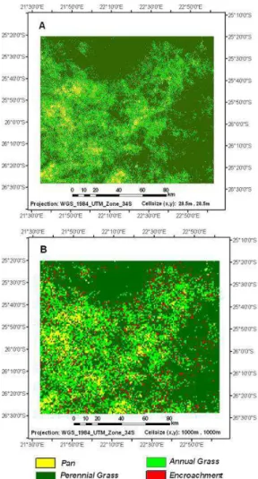
The region where up-scaled NO emissions were calculated is around the town of Tsabong in the southern part of the Kalahari. Up-scaling has been limited to an area the size of a Landsat image (185 km×185 km, see highlighted square in Fig. 1). This is

in the region where the field sampling took place and where the climate and soil

prop-5

erties are fairly homogeneous (Fig. 1). The four corners demarcating the region are (24◦₅₇′_18.51′′_{S, 21}◦₃₆′_20.12′′_{E), (25}◦₀₂′_20.31′′_{S, 23}◦₀₄′_54.75′′_{E); (26}◦₂₆′_58.27′′_S,

21◦34′57.92′′E) and (26◦30′04.40′′S, 23◦05′29.43′′E). The land use for the area was described using high resolution Landsat images in combination with visual interpreta-tion of field condiinterpreta-tions.

10

Multiband Landsat images for May 2000 (Landsat-7 Enhanced Thematic Mapper), positioned within Landsat path 174 row 78, were provided by the US Geological Survey (USGS) (since this is a remote rural region it was assumed that there have be no significant changes in the land use between May 2000 and May 2006). These images were rectified to UTM zone 34 S and image processing was performed using ERDAS

15

Imagine, version 8.7.

Vegetation cover was defined using Normalized Diff_{erence Vegetation Index (NDVI)}

based vegetation rendering since it provides a good spectral characterization parame-ter (Roettger, 2007). The NDVI was calculated using Landsat channels 3 (R: red) and 4 (IR: near infrared) using equation 13:

20

NDVI=IR−R

IR+_R (13)

The NDVI values range from−1 to+1 and correlate with the vegetation cover; high

NDVI values indicate higher biomass (Roettger, 2007) and larger plants, therefore larger vegetation (trees and shrubs) will have a higher NDVI value, while sparse veg-etation and grass have lower values. Bare soil and rocks reflect in the near infrared

25

(17)

there-BGD

5, 4621–4680, 2008

G. T. Feig et al.

Title Page

Tables Figures

◭ ◮

Back Close

Full Screen / Esc

fore have values below zero; however snow and standing water is not expected in this area.

Our classification scheme for the land use was based on the NDVI pixel value and on the “supervised classification approach”, where an analyst selects “training areas” that are spectrally representative of the land cover classes of interest (ERDAS Field

5

Guide by Leica, 2005). In this case the training areas were the vegetation patches chosen at the Berry Bush Farm where the soil samples were taken (three replicates per vegetation patch type). The vegetation patches were delineated in the field with a hand held GPS device. Parametric signatures ware developed from the NDVI values of the pixels in each vegetation patch, based on statistical parameters (maximum, minimum,

10

mean and covariance of the NDVI matrix) of the pixels that are in the training areas at a resolution of 28 m×28 m (which is smaller than the size of the vegetation patches

measured in the field) (Roettger, 2007).

In this study NDVI values ranged from 0.29 to 0.00, which corresponds to “light to sparse vegetation cover and bare soils” (Roettger, 2007).

15

NDVI signatures for each of the patches were defined as 0.0–0.039 for the Pan, 0.040–0.057 for the Annual Grassland, 0.058–0.24 for the Perennial Grassland, and 0.25–0.29 for the Encroachment.

The land use distribution in this part of the Kalahari was later used for estimating the emissions of NO from the soil using MODIS land surface temperature data (LST). This

20

data is provided at a coarser resolution (1 km×1 km) and it was therefore necessary to

change the resolution of the land cover data from 28 m×28 m (Fig. 7a) to that of the

LST (1 km×1 km) (Fig. 7b), this up-scaling procedure was performed in GIS mapping,

where one can accurately estimate block estimates from pixels of smaller resolution.

2.9.2 Soil moisture classification

25

(18)

BGD

5, 4621–4680, 2008

G. T. Feig et al.

Title Page

Tables Figures

◭ ◮

Back Close

Full Screen / Esc

of soil moisture at a 1 km resolution. The project uses the ENVISAT ASAR (Advanced synthetic aperture radar) sensor in the global mode, in conjunction METOP scaterom-eter sensors (Wagner et al., 2008, 2007). The spatial resolution of the SHARE soil moisture data is less than 1 km and the pixel size is 420 m (aggregated to 1×1 km).

The temporal resolution is variable and the satellite generally makes a pass every 3–5

5

days. Here the spatial distribution of soil moisture (in terms of soil Water Filled Pore Space) is mapped using GIS techniques.

2.9.3 Soil temperature classification

Soil surface temperature was obtained from the MODIS (Moderate Resolution Imag-ing Spectroradiometer) land surface temperature products MOD11A2 Eight-Day LST,

10

distributed by the Land Process Distributed Active Archive Centre (LP DAAC) for the period December 2005–November 2006. Land surface temperatures (LST) (corre-sponding to a skin temperature) were obtained using the “screened for cloud eff_ects

and split-windows algorithm” (Wan et al., 2002), and the day/night algorithm which is usually applied to tropical regions (Wan, 2003). The MOD11A2 Eight-day LST is the

15

average land surface temperature over an 8 day period obtained from daily products from the MOD11A1 at a 1 km spatial resolution. The land surface temperatures were mapped for the study area using ENVI 3.6 software. Comparisons of the satellite de-rived surface temperatures were compared with measured soil temperatures (5 depth) at the WMO weather station at Tsabong obtained from the National Climate Data

Cen-20

tre (NCDC) of the National Oceanic and Atmospheric Administration (NOAA).

2.9.4 NO up-scaling

The emission of NO from the soil was calculated for 12 months based on the param-eters obtained from the laboratory flux measurements, distribution of the vegetation patches obtained from Landsat, the soil moisture estimations obtained from the

EN-25

(19)

algo-BGD

5, 4621–4680, 2008

G. T. Feig et al.

Title Page

Tables Figures

◭ ◮

Back Close

Full Screen / Esc

rithm of Meixner and Yang (2006) (see Eq. 11).

3 Results

3.1 Soil physical and chemical properties

The soils in all the vegetation patches have a high sand content of over 70% and the soils are classified as sandy loam soils, except for the Pan soils which are sandy

5

clay loam soils. The mean bulk density of the soils is between 1.4×103kg m−3 and

1.5×103kg m−3and does not differ significantly between the vegetation patches.

The mean pH in the Annual Grassland, Perennial Grassland and Encroachment patches ranges from 6.1–6.5 and does not diff_{er significantly (}_p>_{0.05). However in}

the Pan the mean pH is 8.5 and this is significantly higher than in the other patches

10

(p<0.05). Diff_{erences occur within the Pan patch where the Tree cover has a}

signifi-cantly lower pH than the Open. The pH values are 8.4 and 8.6 for the Tree cover and Open, respectively (p<0.05,n=_3).

There are no significant diff_{erences in the mean total N contents between the}

veg-etation patches, which range from 0.05–0.07% total N; however there are vegveg-etation

15

cover type related diff_{erences (Table 2). In the Encroachment and Perennial}

Grass-land patches where the total N content under Tree cover is significantly higher than under the Open or Grass cover classes (p<0.01,n=_{3). There are no significant di}ff

er-ences (p>0.05) in the total N continents within either the Pan or the Annual Grassland vegetation patches. The total C content of the soil does not diff_{er between the} vegeta-20

tion patches; however diff_{erences occur between the vegetation cover units within the}

patches (Table 2). In the Encroachment patches total C is significantly higher under the Tree cover than under either the Open or Grass cover classes (p<0.05, n=_{3). In}

the Perennial Grassland the total C content under the Tree canopies is significantly higher than under the Grass or Open cover types (p<0.05,n=_{3). In the Annual} Grass-25

(20)

BGD

5, 4621–4680, 2008

G. T. Feig et al.

Title Page

Tables Figures

◭ ◮

Back Close

Full Screen / Esc

(p<0.05, n=_{3) and is greater than under Grass cover at the 10% confidence interval}

(p<0.1, n=_{3). In the Pan patches the soil C content is significantly higher under the}

Tree canopy than under the Open or Crust cover types (p<0.05, n=_{3) and is greater}

than the Grass cover type (p<0.1,n=_3).

3.2 Vegetation cover

5

There are distinct diff_{erences in the vegetation cover patterns between the four chosen}

vegetation patch types.

The Annual Grassland patch was covered by 56% annual grass species, mostly

Schmiditia kalihariensis(Stent). None of the other vegetation patches had a cover of annual grass species as high as the Annual Grassland, the Pan had the next highest

10

cover with 14% annual grass cover.

In the Encroachment patch the vegetation cover was dominated by tree cover, al-most exclusivelyA. melliferasubsp.detinens(Burch.), which made up 37% of the total vegetation cover in the Encroached patch, more than double the 7–15% tree cover in the other patches. The dominant vegetation types in the Perennial Grassland patches

15

were perennial grass species, which made up 25% of the vegetation cover. In the Pan the vegetation composition was fairly evenly distributed between the vegetation func-tional types, however this was the only patch where 2nd or 3rd degree soil crusts made an important contribution to the vegetation cover. In all the vegetation patches there was a large amount of uncovered soil which ranged from 17% in the Annual Grassland

20

to 45% in the Perennial Grassland.

3.3 Laboratory NO flux

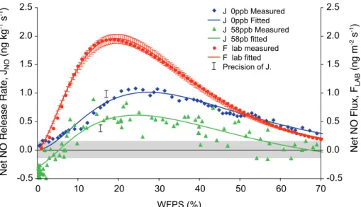
Figure 3 shows an example of the net NO release (J release) values from soils of the Annual Grassland patch and under Grass cover with NO free air incubation,J release under incubation with air containing 58 ppb NO, and the calculated net potential NO

25

(21)

BGD

5, 4621–4680, 2008

G. T. Feig et al.

Title Page

Tables Figures

◭ ◮

Back Close

Full Screen / Esc

indicating that uptake of NO is occurring in the soil, while the shapes of the emission curves are comparable. The flux of NO has slightly diff_{ering optimal soil moisture to}

the two release values due to the position of the areas of NO uptake.

In all the vegetation patches the maximum net potential NO flux was below 5 ng m−2s−1(Fig. 4). The highest net potential NO fluxes occurred from the soils in the

5

Perennial Grassland and Encroachment patches, 4.3 ng m−2s−1(25◦C), 3.1 ng m−2s−1 (35◦C) in the Perennial Grassland, 3.3 ng m−2s−1(25◦C) and 3.3 ng m−2s−1 (35◦C) in the Encroachment Patch. The lowest net potential NO fluxes occurred from the Pan where the NO flux did not exceed 0.6 ng m−2s−1and 1.3 ng m−2s−1at 25◦C and 35◦C, respectively. This indicates that there are diff_{erences between the vegetation patches,} 10

caused either by the soil physical properties or by the diff_{ering vegetation.}

In all the patches, except the Perennial Grassland, the potential NO flux is greater at the 35◦C incubation than the 25◦C incubation. In the Perennial Grassland the potential flux was greater at 25◦_{C, indicating that there is an optimum soil temperature for the}

emission of NO, above which the emissions start to decrease. There is no constant

15

pattern as to which vegetation cover type produces the highest or lowest NO flux, as these change between the diff_{erent vegetation patches and is not even consistent}

un-der the diff_{erent temperature treatments. However at 25}◦_{C the maximum net potential}

NO flux tends to occur under the dominant vegetation cover unit within the vegetation patch.

20

– In the Pan patch the maximum net potential NO flux from under the Crusts (0.6 ng m−2_s−1_{) is more than 25% higher than under any of the other vegetation}

cover units (0.4 ng m−2s−1for Grass and Trees and 0.3 ng m−2s−1for Open);

– In the Annual Grassland the maximum net potential NO flux under Grass cover (1.95 ng m−2s−1) is twice as high as under the highest of the other vegetation

25

cover types (0.9 ng m−2s−1).;

– In the Perennial Grassland patch the maximum net potential NO flux of 4.3 ng m−2

s−1

(22)

BGD

5, 4621–4680, 2008

G. T. Feig et al.

Title Page

Tables Figures

◭ ◮

Back Close

Full Screen / Esc

NO flux from under Trees is 3.2 ng m−2s−1and 2 ng m−2s−1from under the Grass canopy.

– In the Encroachment patch the maximum net potential NO flux from under the Tree canopies (3.3 ng m−2s−1) is between 25% and 50% higher than under the Open (1.6 ng m−2s−1) and Grass cover (2 ng m−2s−1).

5

At 35◦_{C these patterns have changed so that in the Annual Grassland, Perennial}

Grass-land and Encroachment sites the maximum net potential NO flux comes from under the Trees, while in the Pan patch it occurs under the Grass canopy.

The median optimal WFPS (where F_lab is maximum) for all patches and covers at 25◦C is 16.3% (12.4% and 20% for 25 and 75 percentile respectively). At 35◦C

10

the median optimal WFPS is slightly higher at 19.3% WFPS (14.5% and 21.9%, for the 25 and 75 percentile, respectively), although these diff_{erences are not significant}

(p>0.05). Therefore the optimum soil moisture for the emission of NO is fairly low (20%

WFPS=_5.8%Θ_{), as is expected since the production of NO is a result to the aerobic}

process of nitrification.

15

3.4 Mean net potential patch NO flux

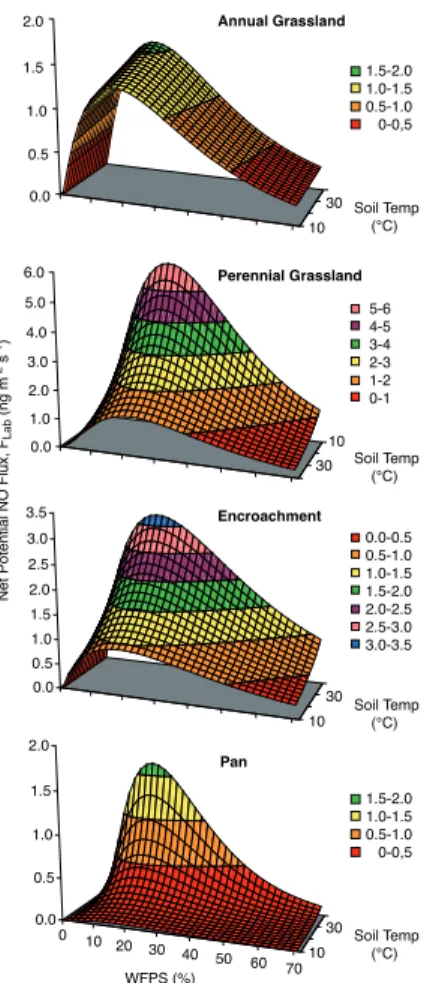
To determine the mean net potential NO flux of an entire patch, the NO flux within each patch have been apportioned from the individual net potential NO fluxes from the corresponding vegetation cover types according to the total coverage of that vegetation cover type (as shown in Fig. 2). This results in mean net potential flux curves for

20

each of the vegetation patches (Fig. 5). The lowest mean net potential NO flux still occurs in the Pan patch where the maxima are less than 0.27 ng m−2s−1 (25◦C) and 0.89 ng m−2s−1(35◦C), respectively. The highest net potential NO flux comes from the Perennial Grassland patch where the maximum flux (2.95 ng m−2s−1) is reached at soil moisture content of 24% soil WFPS and a soil temperature of 25◦C. In all the patches

25

(23)

BGD

5, 4621–4680, 2008

G. T. Feig et al.

Title Page

Tables Figures

◭ ◮

Back Close

Full Screen / Esc

Temperature does not have a consistent influence on the optimal WFPS. In the Pan and Perennial Grassland patches the optimal soil moisture under the two incubation temperatures is approximately the same, however in the Annual Grassland the optimal WFPS is shifted towards dryer soil conditions at the higher incubation temperature and in the Encroachment it is shifted towards wetter conditions under the higher incubation

5

temperatures. The eff_{ect of temperature is also not consistent; in the Pan and}

En-croachment patches an increase in temperature results in a strong increase in net po-tential NO flux. TheQ₁₀value is 3.54 and 1.51 for the Pan and Encroachment patches respectively. However in the Annual Grassland these eff_{ects are not as strong. In the}

Annual Grassland theQ₁₀ value is 1.07 indicating that in the 25◦C to 35◦C

tempera-10

ture range there is virtually no temperature influence on the NO flux. In the Perennial Grassland there is a negative temperature relationship in the 25◦C to 35◦C temperature range (Q₁₀=_{0.61) and as the temperature increases the NO flux decreases.}

Fitting the laboratory measured net potential NO fluxes as a function of both soil moisture and temperature gives the net potential flux curves as shown in Fig. 6. Using

15

these curves an estimate of the net potential NO flux can be made for any known soil water and temperature content.

3.5 NO compensation mixing ratio and NO consumption rate

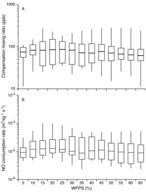
The median NO compensation mixing ratio (25◦C) as a function of soil moisture is shown in Fig. 7a. The medianm_NO_,_comp ranges from 61–86 ppb NO with the highest

20

median values occurring between 20% and 25% WFPS. The lower 25 percentile range is from 35 to 63 ppb NO while the 75 percentile range is from 86 to 147 ppb NO. The m_NO_,_compdoes not seem to be strongly influenced by the soil moisture content (at least not in the range of soil WFPS found in this study Sect. 3.6.2).

The NO consumption rate (k) at 25◦C, calculated from Eq. (3) as a function of WFPS

25

(24)

BGD

5, 4621–4680, 2008

G. T. Feig et al.

Title Page

Tables Figures

◭ ◮

Back Close

Full Screen / Esc

values range from 0.9×10−5m3kg−1s−1 (30%–35% WFPS) to 1.3×10−5m3kg−1s−1

(15%–20% WFPS). The lower 25 percentile ranges from 3.7×10−6(55%–60% WFPS)

to 9.3×10−6m3kg−1s−1 (20%–25% WFPS) and the upper 75 percentile ranges from

1.5×10−5(2.5%–5% WFPS) to 3.4×10−5×10−5m3kg−1s−1(25%–30% WFPS).

3.6 NO up-scaling

5

Up-scaling the NO flux from the corresponding mean net potential NO flux for each of the vegetation patches (see Fig. 6) to the regional scale required three sets of land-scape based information: the vegetation patch distribution; the soil moisture content; and the soil surface temperature.

3.6.1 Vegetation patch distribution

10

Using the Landsat NDVI (see Sect. 2.9.1) provided a high resolution distribution of the vegetation patches (28 m×28 m) in this region (Fig. 1) of the southern Kalahari

(Fig. 8a). The proportion of land cover from each patch type was 60.3% for Perennial Grassland, 26.8% for Annual Grassland, 6.3% for Encroachment and 6.6% for Pan. Decreasing the resolution of the vegetation patch distribution to 1 km×1 km (Fig. 8b)

15

did not result in any major changes in the proportion of land covered by the vegetation patches; percentage distribution was 59.9%, 26.9%, 6.4% and 6.8% for the Perennial Grassland, Annual Grassland, Encroachment and Pan respectively.

3.6.2 Soil moisture

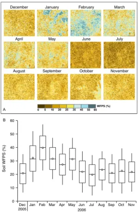
The mean monthly soil WFPS for the up-scaled section of the southern Kalahari for the

20

(25)

BGD

5, 4621–4680, 2008

G. T. Feig et al.

Title Page

Tables Figures

◭ ◮

Back Close

Full Screen / Esc

soil moisture are widely distributed through the region. There was also an increase in the mean soil moisture content between March and May and following rains in October, although in these time periods the soil moisture distribution is patchier and less widely distributed. The soils were driest in July where the mean WFPS in the soils was less than 20%. Spatial diff_{erences exist where small scale convective storms occurred,} 5

creating a patchy distribution of soil moisture through the landscape. These estimates are partly corroborated from gravimetric soil moisture data in a study by (Thomas et al., 2008) which occurred at the Berry Bush Farm in May 2006, which is equivalent to a soil moisture content of 22.5%–34% WFPS (10–15% volumetric soil moisture). The monthly range of the soil moisture contents can be seen in Fig. 10b, where the mean

10

values range from 20% to 48%.

3.6.3 Soil surface temperature

The soil surface temperature for December 2005–November 2006 was obtained from the MODIS instrument at a resolution of 1 km (see Sect. 2.9.3) and is shown in Fig. 10a. Variations can be seen in the land surface temperature values (averaged over 8 days)

15

which range from approx. 13◦C in July (austral winter) to 47◦C in January (austral sum-mer). While some spatial diff_{erences occur across the landscape the spatial distribution}

is not as marked as those found in the soil moisture distribution. Figure 10b shows a comparison between the surface temperature obtained for the Tsabong area using the remote sensing technique and the measured mean monthly temperature measured at

20

(26)

BGD

5, 4621–4680, 2008

G. T. Feig et al.

Title Page

Tables Figures

◭ ◮

Back Close

Full Screen / Esc

3.6.4 Up-scaled NO fluxes

The up-scaled NO flux for the selected part of the southern Kalahari is presented in Fig. 11a. The up-scaled mean monthly flux of NO ranges from 0–323 g ha−1_month−1

(0 to 13.6 ng m−2s−1) over the course of the year. The highest emissions of NO oc-curred from the least disturbed of the vegetation types, the Perennial Grassland where

5

the emissions of NO reached a maximum of 323 g ha−1month−1 in some of the pix-els in February 2006, although the largest mean NO emission was 240 g ha−1month−1 (9.9 ng m−2vs−1) for February 2006. The next highest rate of NO emission occurred in the Encroached sites where the flux of NO reached a maximum of 143 g ha−1month−1 (5.4 ng m−2s−1) and the largest mean flux was 124 g ha−1month−1 (4.6 ng m−2s−1) in

10

January 2006. In the Annual Grassland vegetation patches the greatest mean monthly NO flux was 119 g ha−1month−1 (2.0 ng m−2s−1) while a maximum pixel value of 216 g ha−1month−1(3.6 ng m−2s−1) was recorded in March 2006. Mean up-scaled NO fluxes were lowest in the Pan patches and the largest mean flux was 33 g ha−1month−1 (1.4 ng m−2s−1) in February 2006 while the highest pixel value was 60 g ha−1month−1

15

(3.15 ng m−2

s−1

) which occurred in March 2006. The maximum up-scaled flux was reached in the austral summer where the greatest biogenic emissions of NO were pro-duced in the warm, moist month of February. The lowest NO fluxes occurred in the austral winter months where the soil temperature and moisture content were at the lowest in the annual cycle. During June, July and August the flux of NO out of the soil

20

in these ecosystems is negligible (in July 2006, the maximum NO flux was less than 1.8 g ha−1_month−1_).

4 Discussion

This study has tried to up-scale the emissions of NO from diff_{ering vegetation patches}

in an arid Kalahari savanna. During the course of the study three main aspects were

25

(27)

BGD

5, 4621–4680, 2008

G. T. Feig et al.

Title Page

Tables Figures

◭ ◮

Back Close

Full Screen / Esc

1. The soil physical and chemical properties, including the soil texture, pH the total N and C contents.

2. The net potential NO flux, which was measured in the laboratory and examines both inter and intra patch diff_erences

3. The NO flux up-scaled to a region the size of a Landsat image (185 km×185 km)

5

using a combination of remote sensing techniques.

4.1 Soil physical and chemical properties

In this study we recorded soil textures consisting of 71–79% sand, 3.8–7.6% silt and 16.5–21% clay (see Table 1). Diff_{erences in the soil textural classes between the Pan}

and the other vegetation patches has been previously noticed, while soil textures of the

10

Perennial Grassland, Encroachment and Annual Grassland are typical of the Kalahari sands. The Pan patches have more clayey soil and are more calcareous resulting in a higher pH (van Rooyen and van Rooyen, 1998).

The mean total soil C and total N values reported in this study (see Table 2) range from 0.2%–1% total C and from 0.03%–0.12% total N. These are at the lower end of

15

values reported from the Kalahari in other studies, where the soil C ranges from 0.2% to 6% (Aranibar et al., 2004; Dougill et al., 1998; Feral et al., 2003) and the reported soil N contents range from 0.025–0.045% (Aranibar et al., 2004). Few diff_{erences in}

the mean soil chemical properties between the diff_{ering patches occurred, however}

there were diff_{erences within each of the patches.} 20

In this study, diff_{erences in the soil chemical properties were found under di}ff_ering

vegetation cover units within each of the patches. In most of the vegetation patches the total soil C and total soil N were higher under tree canopies than away from the canopies. This has also been found in other studies (Dougill and Thomas, 2004; Hagos and Smit, 2005). The diff_{erences in soil nutrient concentration under the tree canopies} 25

(28)

BGD

5, 4621–4680, 2008

G. T. Feig et al.

Title Page

Tables Figures

◭ ◮

Back Close

Full Screen / Esc

by members of theMimosaceae family all of them within theAcaciagenus. The Aca-ciagenus is known to undergo the process of biological nitrogen fixation (Dougill and Thomas, 2002; Scholes and Walker, 1993; Schulze et al., 1991). It has also been pro-posed that the “island of fertility eff_{ect” is due to nutrients being trapped by plant stems}

and root systems (Aranibar et al., 2004; Hagos and Smit, 2005; Ludwig and Tongway,

5

1995; Ludwig et al., 1999; Tongway et al., 1989).

The results of the soil physical and chemical investigations show that all the vegeta-tion patches, apart from the Pan soils, can be considered to be on a fairly homogenous substrate shown by the similarity in the soil textural properties, soil pH and the to-tal C and N contents of the soil (Aranibar et al., 2004; Scholes et al., 2002), however

10

there are micro-scale diff_{erences in the soil physical and chemical properties due to the}

presence of diff_{ering vegetation cover. These micro-scale di}ff_{erences are what drive}

the variation in biological processes between the vegetation patches and as a result are likely to influence the net potential NO flux from the soil.

4.2 Net potential NO flux

15

This is the fifth study of the biogenic emissions of NO from soils in savanna ecosystems of southern Africa, which has been conducted using a similar laboratory technique. Other studies include:

– The Nylsvley Savanna where the flux on NO ranged from 0.12 ng m−2s−1 to 13.86 ng m−2s−1 with mean and median values of 2.89 ng m−2s−1 and

20

0.90 ng m−2_s−1_{respectively (Otter et al., 1999).}

– Miombo savannas and grasslands in Zimbabwe where the NO flux ranged from 0.5 ng−2s−1 to 9.4 ng m−2s−1 with mean and median values of 2.93 ng m−2s−1 and 1.1 ng m−2s−1respectively (Kirkman et al., 2001).

– The Botswana Kalahari Transect where the values ranged from 8 ng m−2s−1 to

25

(29)

BGD

5, 4621–4680, 2008

G. T. Feig et al.

Title Page

Tables Figures

◭ ◮

Back Close

Full Screen / Esc

respectively (Aranibar et al., 2004).

– Landscape in the Kruger National Park in South Africa where the NO flux ranged from 0.06 ng m−1s−1 to 3.52 ng m−1s−1 and mean and median values were 1.67 ng m−2s−1and 1.63 ng m−2s−1respectively (Feig et al., 2008).

The net potential NO fluxes calculated for the diff_{ering vegetation patches in this study} 5

(0–3.5 ng m−2s−1) correspond very well with the values previously reported by Otter (1999), Kirkman (2001) and Feig (2008). The reasons why the Aranibar et al. (2004) study gave such diff_{ering results is unclear and the causes cannot currently be judged.}

In other natural arid and semi-arid regions (mean annual precipitation <700 mm) the measured median NO fluxes range from 0.07 ng m−2s−1to 5.3 ng m−2s−1(with

re-10

ported values of up to 83 ng m−2s−2 occurred during a pulsing event, such as when the soil is wetted or fertilized) (Davidson et al., 1993; Feig et al., 2008; Hartley and Schlesinger, 2000; Holst et al., 2007; Martin and Asner, 2005; Martin et al., 1998; McCalley and Sparks, 2008; Smart et al., 1999). The NO fluxes from these arid and semi-arid ecosystems tend to be fairly low in comparison with some of the values

re-15

ported from temperate and tropical forests where fluxes of 22 ng m−2s−1(Pilegaard et al., 2006) and 58 ng m−2s−1(Butterbach-Bahl et al., 2004) were reported in European coniferous and Australian tropical forests respectively.

4.3 Intra and inter patch variability

Within each of the vegetation patches diff_{erences in the net potential NO flux occurred} 20

under the diff_{erent vegetation cover types, although the patterns were not consistent}

between the vegetation patches either due to the soil nutrient status or due to changes in the microclimates under diff_{ering vegetation cover types.}

Once the mean net potential NO flux was determined for each of the vegetation patches (by incorporating the proportion of diff_{erent cover units within each of the} veg-25

etation patch types) it could be seen that diff_{erences in the mean net potential fluxes of}