Comparative Study of Backpropagation Algorithms in Neural Network Based Identification of Power System

COMPARATIVE STUDY OF

BACKPROPAGATION

ALGORITHMS IN

NEURAL

NETWORK BASED

IDENTIFICATION OF

POWER

SYSTEM

Sheela Tiwari

, Ram Naresh

, Rameshwar Jha

1

Department of Instrumentation and Control Engineering, Dr. B R Ambedkar National Institute of Technology, Jalandhar, Punjab, India

tiwaris@nitj.ac.in 2

Department of Electrical Engineering, National Institute of Technology, Hamirpur, Himachal Pradesh, India

rnareshnith@gmail.com 3

IET Bhaddal Technical Campus, Ropar, Punjab, India rjharjha@yahoo.com

A

This paper explores the application of artificial neural networks for online identification of a multimachine power system. A recurrent neural network has been proposed as the identifier of the two area, four machine system which is a benchmark system for studying electromechanical oscillations in multimachine power systems. This neural identifier is trained using the static Backpropagation algorithm. The emphasis of the paper is on investigating the performance of the variants of the Backpropagation algorithm in training the neural identifier. The paper also compares the performances of the neural identifiers trained using variants of the Backpropagation algorithm over a wide range of operating conditions. The simulation results establish a satisfactory performance of the trained neural identifiers in identification of the test power system.

K

System Identification, Recurrent Neural Networks, Static Backpropagation (BP)

1. I

[7] and in protection strategies [8-9]. Applications of ANNs in reactive power transfer allocation [10] and ATC estimation [11] have been reported. Stability issues like damping of oscillations [12-14], prediction of loadability margins [15] and voltage contingency screening [16] have been successfully addressed by ANN based solutions. ANNs have the potential of application for real-time control [17]. Accurate system identification is of immense importance in power system operation and control. The capabilities of the ANNs make them a suitable choice for this application. Multilayer feedforward artificial neural networks using Backpropagation algorithm for training have been proposed for successful online model identification of synchronous generator [18] and a UPFC equipped single machine infinite bus system [19]. A neural network based estimation unit has been proposed to estimate in real time, the parameters for an interfacing scheme for grid-connected inverters and simultaneously estimating the grid voltage [20]. The authors have employed neural network for system identification for predictive control of a multimachine power system operating under widely varying operating conditions and subjected to transient conditions [21].

The work undertaken proposes to use a recurrent neural network for online identification of a multimachine power system. Since the Backpropagation algorithm has been successfully employed to train system identifiers as already reported in literature [18-19], this work aims to investigate the training performance of some of the variants of the Backpropagation algorithm in training the proposed neural identifier. The testing performances of the neural identifiers trained using variants of the Backpropagation algorithm are also compared to establish the accuracy of the differently trained identifiers.

This paper is organized as: Section 2 presents a brief overview of the recurrent neural networks including the types of architecture for training such networks. Section 3 describes the system under consideration and outlines the objectives of this work. Section 4 presents the architecture of the proposed neural identifier. Section 5 discusses the training of the proposed identifier and presents a brief overview of the variants of the Backpropagation algorithm used for training the proposed neural identifier in this work. The simulation results of training and testing the proposed identifier and the discussions are presented in section 6 followed by the conclusions in section 7.

2. RECURRENT NEURAL NETWORKS

Neural networks are broadly classified as static networks and dynamic networks. In case of static networks, the output of the network is dependent only on the current input to the network and is calculated directly from the input passing through the feedforward connections. There are no delay elements and no feedback elements present in the static networks. In dynamic networks, the output of the network depends on the current input as well as on current and/or previous inputs and outputs i.e. states of the network. These networks therefore, are said to possess memory and can be trained to learn sequential or time varying patterns [22], making them more powerful than the static networks. Dynamic networks are further divided into two categories: those having only feedforward connections with delays at the input layer only/or distributed throughout the network and those having feedback or recurrent connections.

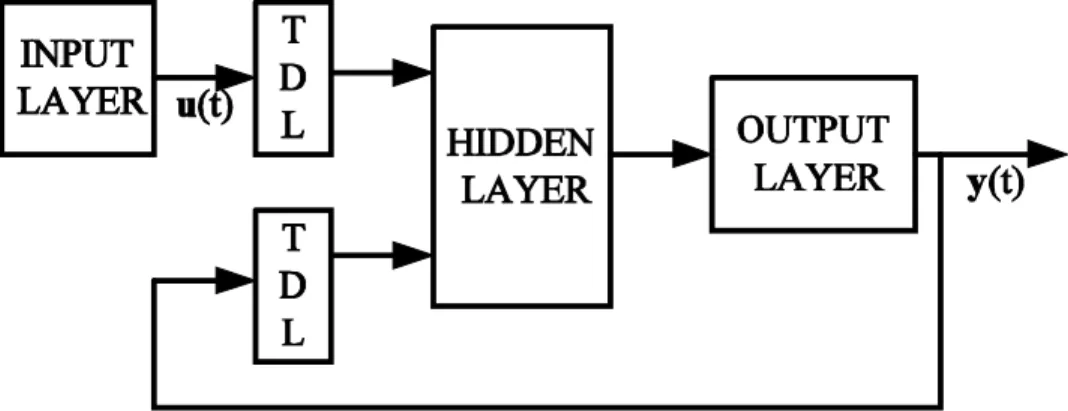
Where y(k) and u(k) are the outputs and inputs at the kth instant and nyand nuare the number of time steps for which the current output is regressed on the output and input respectively. A diagram showing the implementation of the NARX model using a feedforward neural network to approximate the function f in (1) is given in Figure 1.

Two different architectures have been proposed to train a NARX network [22]. First is the parallel architecture as shown in Figure 2, where the output of the neural network is fed back to the input of the feedforward neural network as part of the standard NARX architecture. In contrast, in the series-parallel architecture as shown in Figure 3, the true output of the plant (not the output of the identifier) is fed to the neural network model as it is available during training. This architecture has two advantages [22]. The first is a more accurate value presented as input to the neural network. The second advantage is the absence of a feedback loop in the network thereby enabling the use of static backpropagation for training instead of the computationally expensive dynamic backpropagation required for the parallel architecture. Also, assuming the output error tends to a small value asymptotically so that , the series parallel

model may be replaced by a parallel model without serious consequences if required.

Figure 1. Implementation of NARX model

Figure 3. Series-Parallel architecture of training a NARX model

3. SYSTEM DESCRIPTION

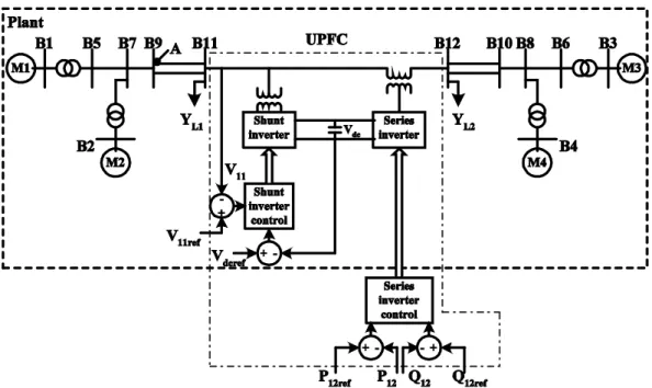
The two area, four machine system with active power flowing from Area 1 to Area 2 [23], proposed to study the electromechanical oscillations of a multimachine power system is taken as the test system for the work undertaken. In spite of the small size of the system, its behaviour mimics the behaviour of a large power system in actual operation. Each area comprises of two 900 MVA machines and the two areas are connected by a 220 kV double circuit line of length 220 km. The load voltage profile is improved by installing additional 187 MVAr capacitors in each area. The system under study is equipped with PSS and has a UPFC installed between bus 11 and bus 12 with bus 11 common to the shunt and series converters and the other side of the series converter connected to bus 12 as shown in Figure 4.

Figure 4. 2-Area system equipped with UPFC

injected by the UPFC is to be predicted under various operating conditions. This next step value of is predicted using the values of and at some preceding instants.

Objectives

i. To design a neural identifier to predict the next step value of on the basis of the

values of and at preceding time instants.

ii. To investigate the performances of the variants of the Backpropagation algorithm for training the neural identifier.

iii. To investigate the performances of the neural identifiers trained using the variants of the Backpropagation algorithm.

iv. To propose the most suitable of the considered variants of the Backpropagation algorithm for online application for the system under consideration.

4. ARCHITECTURE OF THE NEURAL IDENTIFIER

A neural identifier that predicts the next step value of on the basis of the values of and

at four preceding instants is proposed. As the objective clearly requires a dynamic neural network, the NARX model is used. A two layer neural network with sigmoidal hidden layer neurons and linear output layer neurons can identify any system with any degree of accuracy, subject to the availability of sufficient number of hidden neurons [24]. Therefore, the NARX model is implemented using the two layer feedforward neural network. Since the true value of the output for the preceding instants are available, the series parallel architecture is used. As the values of and at four preceding instants are to be used, the total number of inputs to the

neural network is eight as shown in Figure 5. The number of sigmoidal neurons in the hidden layer has been fixed at thirteen using trial and error approach and the output layer has one linear neuron.

The system under consideration is modelled and simulated using MATLAB / SIMULINK to generate data for training and testing the proposed neural identifier. The operation of the system is simulated by applying restricted within the range +0.1 pu and -0.1 pu (restricting the quadrature component of the series injected voltage to 10% of the nominal line-to-ground voltage) and sampling the input, and output, at the rate of 32 samples per second. The neural network is presented with the following inputs

And

for predicting For linear input neurons, the output of the input neurons is same as the input given by

The output of the hidden layer (layer 1), consisting of 13 sigmoidal neurons is given by

Where, is the weight matrix between input and hidden layers and is the bias to the hidden layer neurons. Similarly, the output of the output layer (layer 2), comprising of one linear neuron is given by

Where, is the weight matrix between hidden and output and layers and is the bias to the output layer neurons.

5. TRAINING OF THE NEURAL IDENTIFIER

Identification requires setting up a suitably parameterized identification model and adjustment of these parameters of the model to optimize a performance function based on the error between the outputs from the plant and the identification model [22]. It is assumed that the weight matrices of the neural network proposed as the identifier exists, for which, both plant and the identifier have the same output for any specified inputs, for the same initial conditions [22].

Where, N is the size of the training dataset, and are the target and predicted value of the

output of the neural network when the input is presented and is the error (difference

between the target and predicted value) for the input. The performance index V in (7) is a

function of weights and biases, and can be given by

The performance of the neural network can be improved by modifying till the desired level of

the performance index, is achieved. This is achieved by minimizing with respect to and the gradient required for this is given by

where, is the Jacobian matrix given by

and is the error for all the inputs. The gradient in (9) is determined using backpropagation, which involves performing computations backward through the network. This gradient is then used by different algorithms to update the weights of the network. These algorithms differ in the way they use the gradient to update the weights of the network and are known as the variants of the Backpropagation algorithm.

This work compares the performance of the basic implementation of the Backpropagation algorithm i.e. Gradient descent algorithm with other variants in order to investigate the potentials of these algorithms for online applications in power system identification. A brief overview of the different algorithms considered in this work is given under:

i) Gradient Descent algorithm (GD): The network weights and biases, is modified in a direction that reduces the performance function in (8) most rapidly i.e. the negative of the gradient of the performance function [25]. The updated weights and biases in this algorithm are given by

ii) Scaled Conjugate Gradient Descent algorithm (SCGD): The gradient descent algorithm updates the weights and biases along the steepest descent direction but is usually associated with poor convergence rate as compared to the Conjugate Gradient Descent algorithms, which generally result in faster convergence [26]. In the Conjugate Gradient Descent algorithms, a search is made along the conjugate gradient direction to determine the step size that minimizes the performance function along that line. This time consuming line search is required during all the iterations of the weight update. However, the Scaled Conjugate Gradient Descent algorithm does not require the computationally expensive line search and at the same time has the advantage of the Conjugate Gradient Descent algorithms [26]. The step size in the conjugate direction in this case is determined using the Levenberg-Marquardt approach. The algorithm starts in the direction of the steepest descent given by the negative of the gradient as

The updated weights and biases are then given by

Where, is the step size determined by the Levenberg-Marquardt algorithm [27]. The next search direction that is conjugate to the previous search directions is determined by combining the new steepest descent direction with the previous search direction and is given by

The value of is as given in [26], by

Where is given by

iii) Levenberg-Marquardt algorithm (LM): Since the performance index in (8) is sum of squares of non linear function, the numerical optimization techniques for non linear least squares can be used to minimize this cost function. The Levenberg-Marquardt algorithm, which is an approximation to the Newton’s method is said to be more efficient in comparison to other methods for convergence of the Backpropagation algorithm for training a moderate-sized feedforward neural network [27]. As the cost function is a sum of squares of non linear function, the Hessian matrix required for updating the weights and biases need not be calculated and can be approximated as

Where, μ is a scalar and I is the identity matrix.

iv) Automated Bayesian Regularization (BR):Regularization as a mean of improving network generalization is used within the Levenberg-Marquardt algorithm. Regularization involves modification in the performance function. The performance function for this is the sum of the squares of the errors and it is modified to include a term that consists of the sum of squares of the network weights and biases. The modified performance function is given by

Where SSE and SSW are given by

Where, is the total number of weights and biases, in the network. The performance index

in (19) forces the weights and biases to be small, which produces a smoother network response and avoids over fitting. The values of α and β are determined using Bayesian Regularization in an automated manner [28-29].

6. SIMULATION RESULTS AND DISCUSSION

6.1. TRAINING

The neural network proposed in section 4 was trained using the training set and the training algorithms described in section 5. A Pentium (R) Dual-Core CPU T4400 @2.20 GHz was used to train the proposed neural identifier. Table 1 summarizes the results of training the proposed network using the four training algorithms discussed in the earlier section. Each entry in the table represents 50 different trials, with random initial weights taken for each trial to rule out the weight sensitivity of the performance of the different training algorithms. The network was trained in each case till the value of the performance index in (8) was 0.0001 or less.

Table 1 Statistical comparison of different training algorithms

S. No. Training Algorithm Average

Time (s) Ratio

Maximum Time (s)

Minimum

Time (s) Std Dev.

1. Gradient Descent Very slow in converging

2. Scaled Conjugate

Gradient Descent 280.8473 47.865 911.5366 114.2788 180.7087

3. Levenberg Marquardt 5.8675 1 9.4187 2.9393 1.6995

4. Bayesian

The Gradient Descent algorithm was very slow in converging for the required value of the performance index. The average time required for training the network using the Levenberg-Marquardt algorithm was the least whereas, maximum time was required for training the network using the Scaled Conjugate Gradient Descent algorithm. The training algorithm employing Bayesian Regularization continuously modifies its performance function and hence, takes more time as compared to the Levenberg-Marquardt algorithm but this time is still far less than the Scaled Conjugate Gradient Descent method. From Table 1, it can be established that the Levenberg-Marquardt algorithm is the fastest of all the training algorithms considered in this work for training a neural network to identify the multimachine power system. Since the training time required for different training algorithms have been compared, the conclusion drawn from the results for the offline training may also be extended to online training. Therefore, it can be assumed that similar trend of training time required by the different training algorithms will be exhibited during online training of the proposed neural identifier for continuous updating of the offline trained identifier.

6.2. TESTING

The neural networks trained using the training algorithms listed in Table1 were tested on the same CPU. The test datasets consisted of data points not included in the training set. The system under consideration was simulated at two such operating points for which no data point was included in the training set. The operation of the multimachine power system under consideration at these two operating points was simulated using MATLAB/SIMULINK for a period of 13 seconds each. This period also included a 3-phase short circuit fault at point A at t=10 s for a duration of 200 ms with the circuit breakers auto reclosing after 12 cycles. The data during these two simulations was sampled at the rate of 32 samples per second to form two test sets: Test Set I and Test Set II, corresponding to the two operating points. As the Gradient Descent algorithm was too slow to converge for the desired value of the performance index, the neural networks that were trained using the rest of the three training algorithms listed in Table 1 were tested using these two test sets.

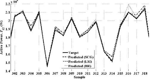
Figure 6. Actual and predicted values of output power during steady state for test set I

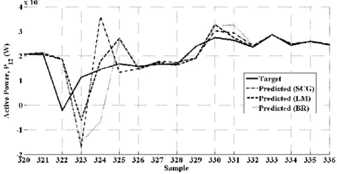
Figure 6 clearly shows that the predictive quality of all the neural networks is satisfactory during the steady state period. The effect of the 3-phase short circuit fault on the system is captured in the sample point 322 of the actual output power as shown in Figure 7. However, the

Figure 7. Actual and predicted values of output power during transient period for test set I

neural networks is investigated by comparing the average absolute error in the predicted values. Table 2 shows the average absolute error along with the maximum error and the minimum error in the values predicted by the trained neural networks.

Table 2 Performance of trained neural networks on test set I

S. No. Training Method

Average Absolute

Error for entire set

Maximum

Error

Minimum

Error

1. SCG 0.0117 1.0689 1.4809e-5

2. LM 0.0103 0.9960 1.0254e-5

3. BR 0.0171 1.8511 7.0297e-6

The average absolute error is the least for the neural network trained using the LM method. The maximum error for every neural network is reported in the transient period and is least for the network trained using the LM method. The neural network trained using the BR method follows the actual values satisfactorily but has slightly higher values of average absolute error and maximum error associated with it as compared to the first two methods. However, the BR method imparts generalization to the network and the neural network trained using BR reported the least minimum error for this test set.

Test Set II: This test set also consists of 417 data points sampled during simulation of the system at an operating point for which the active power flowing in the system at steady state is 156 MW, which is outside the range of active powers flowing at steady state corresponding to the operating points considered for generating the training set. For the same reasons as for Test Set I, the number of predicted values in Test Set II is also 413. In this case too, a 3-phase short circuit fault of duration 200 ms is simulated at t=10 s. Figures 8 and 9 show the actual and predicted output values for a section of steady state and transient period of the system respectively, at the operating point under consideration.

Figure 9. Actual and predicted values of output power during transient period for test set II It is clear from Figure 8 that the actual power output values and the values predicted using the different neural networks in steady state are in close proximity even at this operating point. The decrease in the actual value for the active power immediately after the 3-phase short circuit fault is captured in sample 321 of Figure 9. This information is used by all the neural networks for making predictions for the next instant and all the neural networks successfully predict the decrease in the active power with the minimum power value predicted for sample 322. Similarly, the effect of autoreclosing of the circuit breakers is also predicted successfully by the three neural networks. The average absolute error along with the minimum and maximum errors in the values predicted by the trained neural networks are given in Table 3.

Table 3 clearly shows that the average absolute errors even at such an operating point for which the steady state active power flowing in the system is outside the range of the active powers flowing at operating points considered for generation of training data set are following the same trend as reported in case of Test Set I.

Table 3 Performance of trained neural networks on test set II

S. No. Training Method

Average Absolute Error for entire set

Maximum Error

Minimum Error

1. SCG 0.0092 0.7465 9.9872e-6

2. LM 0.0078 0.5507 1.2711e-5

3. BR 0.0105 0.6905 2.8250e-6

7. CONCLUSION

The fast convergence teamed with good predictive quality makes Levenberg-Marquardt algorithm the most suitable choice of all the variants considered in this work for training a neural network for this application.

R

[1] Halpin, S.M. & Burch, R.F.,(1997) “Applicability of neural networks to industrial and commercial power systems: a tutorial overview”, IEEE Trans. Industry Applications, Vol. 33, No. 5, pp1355-1361.

[2] Hsiung, C.L., (2007) “Intelligent Neural Network-Based Fast Power System Harmonic Detection”,

IEEE Trans. Industrial Electronics, Vol. 54, No. 1, pp43-52.

[3] Mazumdar, J., Harley, R.G., Lambert, F.C., & Venayagamoorthy, G.K., (2007) “Neural Network Based Method for Predicting Nonlinear Load Harmonics”,IEEE Trans. Power Electronics, Vol. 22, No. 3, pp1036-1045.

[4] Mazumdar, J., Harley, R.G., Lambert, F.C., Venayagamoorthy, G.K., & Page, M.L., (2008)

“Intelligent Tool for Determining the True Harmonic Current Contribution of a Customer in a Power Distribution Network”,IEEE Trans. Industry Applications, Vol. 44, No. 5, pp1477-1485.

[5] Cardoso, G., Rolim, J.G., & Zurn, H.H., (2004) “Application of neural-network modules to electric power system fault section estimation”,IEEE Trans. Power Delivery, Vol. 19, No. 3, pp1034- 1041. [6] Cardoso, G., Rolim, J.G., & Zurn, H.H., (2008) “Identifying the Primary Fault Section After

Contingencies in Bulk Power Systems”,IEEE Trans. Power Delivery, Vol. 23, No. 3, pp1335-1342. [7] Liangyu Ma, Yongguang Ma, & Lee, K.Y., (2010) “An Intelligent Power Plant Fault Diagnostics for

Varying Degree of Severity and Loading Conditions”,IEEE Trans. Energy Conversion, Vol. 25, No. 2, pp546-554.

[8] Negnevitsky, M., & Pavlovsky, V., (2005) “Neural networks approach to online identification of multiple failures of protection systems”,IEEE Trans. Power Delivery, Vol. 20, No. 2, pp588- 594. [9] Thalassinakis, E.J., Dialynas, E.N., & Agoris, D., (2006) “Method Combining ANNs and Monte

Carlo Simulation for the Selection of the Load Shedding Protection Strategies in Autonomous Power Systems”,IEEE Trans. Power Systems, Vol. 21, No. 4, pp1574-1582.

[10] Mustafa, M.W., Khalid, S.N., Shareef, H., & Khairuddin, A., (2008) “Reactive power transfer allocation method with the application of artificial neural network”, IET Proc.- Genr. Transm. Distrib., Vol. 2, No. 3, pp402-413.

[11] Pandey, S.N., Pandey, N.K., Tapaswi, S., & Srivastava, L., (2010) “Neural Network-Based Approach for ATC Estimation Using Distributed Computing”, IEEE Trans. Power Systems, Vol. 25, No. 3, pp1291-1300.

[12] Changaroon, B., Srivastava, S.C., & Thukaram, D., (2000) “A neural network based power system stabilizer suitable for on-line training-a practical case study for EGAT system”,IEEE Trans. Energy Conversion, Vol. 15, No. 1, pp103-109.

[13] Chao Lu, Si, J., & Xiaorong Xie., (2008) “Direct Heuristic Dynamic Programming for Damping Oscillations in a Large Power System”, IEEE Trans. Systems, Man, and Cybernetics, Part B: Cybernetics, Vol. 38, No. 4, pp1008-1013.

[14] Nguyen, T.T., & Gianto, R., “Neural networks for adaptive control coordination of PSSs and FACTS devices in multimachine power system”,IET Proc.- Genr. Transm. Distrib., Vol. 2, No. 3, pp355-372. [15] Gu, X., & Canizares, C.A., (2007) “Fast prediction of loadability margins using neural networks to

approximate security boundaries of power systems”,IET Proc.- Genr. Transm. Distrib., Vol. 1, No. 3, pp466-475.

[16] Jain, T., Srivastava, L., & Singh, S.N., (2003) “Fast voltage contingency screening using radial basis function neural network”,IEEE Trans. Power Systems, Vol. 18, No. 4, pp1359- 1366.

[17] Ray, S., & Venayagamoorthy, G.K., (2008) “Real-time implementation of a measurement-based adaptive wide-area control system considering communication delays”, IET Proc.- Genr. Transm. Distrib., Vol. 2, No. 1, pp62-70.

[18] Jung-Wook Park, Venayagamoorthy, G.K., & Harley, R.G., (2005) “MLP/RBF neural-networks-based online global model identification of synchronous generator”, IEEE Trans. Industrial Electronics, Vol. 52, No. 6, pp1685- 1695.

[20] Mohamed, Y.A.-R., & El-Saadany, E.F., (2008) “Adaptive Discrete-Time Grid-Voltage Sensorless Interfacing Scheme for Grid-Connected DG-Inverters Based on Neural-Network Identification and Deadbeat Current Regulation”,IEEE Trans. Power Electronics, Vol. 23, No. 1, pp308-321.

[21] Tiwari, S., Naresh, R., & Jha, R., (2011) “Neural network predictive control of UPFC for improving transient stability performance of power system”,Appl Soft Comput, Vol. 11, No. 8, pp4581-4590. [22] Narendra, K.S., & Parthasarathy, K., (1990) “Identification and control of dynamical systems using

neural networks”,IEEE Trans. Neural Networks, Vol. 1, No. 1, pp4-27.

[23] Kundur, P (1994)Power System Stability and Control, Tata McGraw-Hill, New Delhi.

[24] Hagan, M.T., & Demuth, H.B., (1999) “Neural networks for control”,American Control Conference. [25] Hagan, M.T., Demuth, H.B., & Beale, M.H (1996)Neural Network Design, MA: PWS Publishing,

Boston.

[26] Moller, M.F., (1993)“A scaled conjugate gradient algorithm for fast supervised learning”, Neural Networks, Vol. 6, pp525-533.

[27] Hagan, M.T., & Menhaj, M., (1994) “Training feed-forward networks with the Marquardt algorithm”,

IEEE Trans. Neural Networks, Vol. 5, No. 6, pp989-993.

[28] Foresee, F.D. & Hagan, M.T., (1997) “Gauss-Newton approximation to Bayesian regularization”,

International Joint Conference on Neural Networks.

[29] Mackay, D.J.C., (1992)“Bayesian interpolation”, Neural Computation, Vol. 4, No. 3, pp415-447.

Authors

Sheela Tiwari did her B.E. (Electrical Engineering) from Thapar Institute of Engineering and Technology, Patiala, India in 1993 and M.Tech. in Instrumentation and Control from Department of Electrical Engineering, Punjab Agricultural University in 1996. She joined Regional Engineering College Jalandhar (now Dr. B. R. Ambedkar National Institute of Technology, Jalandhar) as lecturer in the Department of Instrumentation and Control Engineering in 1997 and is currently working as Associate Professor in the same department. Her research interests are artificial intelligence and its application in power systems.

Dr R. Naresh was born in Himachal Pradesh, India in 1965. He received BE in Electrical Engineering from Thapar Institute of Engineering and Technology, Patiala, India in 1987, ME in Power Systems from Punjab Engineering College, Chandigarh in 1990 and Ph D from the University of Roorkee, Roorkee (now IIT Roorkee), India in 1999. He joined Regional Engineering College, Hamirpur (now NIT Hamirpur) in 1989, worked as Assistant Professor in the Department of Electrical Engineering from 2000 to 2007 and is working as Professor in the same department since August

2007. He has taught courses in basic electrical engineering, power systems, electrical machines and artificial neural networks. He has published a number of research papers in national & international journals. He has been providing consultancy services to electric power industry. His research interests are artificial intelligence applications to power system optimization problems, evolutionary computation, neural networks and fuzzy systems.

Dr. R. Jha was born in Bihar, India in 1945. He did B.Sc Engg. (Electrical Engg.) from Bhagalpur Univ. Bhagalpur in 1965, M. Tech. in Control and Instrumentation Engg. from IIT, New Delhi in 1970 and Ph.D in Electrical Engg. in 1980. He served as a Lecturer in Electrical Engg. at Jorhat Engineering College, Jorhat (Assam) from 1965 till he joined as Asstt. Prof. at Panjab Engineering College, Chandigarh in 1972. He joined as Professor of Electrical Engg. at REC Hamirpur (now NIT Hamirpur) in 1986 and was elevated to the post of Principal of REC Hamirpur in 1990 which he continued till 1994. He joined the Department of Instrumentation & Control Engineering at National Institute of Technology Jalandhar as Professor in September