Large Eddy Simulation of Wind Events
Propagating through an Array of Wind Turbines
Rupert Storey, Stuart Norris, and John Cater,
Member, IAENG
Abstract—Large-eddy simulation has been used to model the atmospheric boundary layer flowing through a span-wise periodic array of wind turbines. The wind turbines are modelled using a coupled simulation in which the FAST wind turbine sim-ulation code from NREL operates within a CFD environment. The wind turbines are implemented in the flow-field using the actuator sector technique, and operate dynamically with pitch and yaw control. The development of wind event models for a CFD flow domain is discussed. The cases of a gust event and direction change passing through the farm is simulated, with the resulting flow field through the turbine array and turbine performance examined. The gust model simulations show the propagation of the structure through the array and its resulting dispersion due to the turbine wakes and ambient turbulence. Results from the wind shift simulations show a coherent wind shift front propagating through the domain at the free-stream wind-speed and the action of the yaw controller.
Index Terms—LES, gusts, wakes, wind shifts
I. INTRODUCTION
S
IMULATING wind turbine operation under variousop-erating conditions is a central process in turbine loading and performance predictions. This analysis requires the mod-elling of the dynamics of the wind turbine plant as well as the wind environment to which the turbine is responding. The latter presents several difficulties due to its transient nature and complex driving forces.
For an isolated wind turbine operating in the atmospheric boundary layer (ABL), the wind environment can be mod-elled using a logarithmic velocity profile with turbulent fluctuations superimposed [1]. Grouping of turbines into arrays of farms is common practice to utilise available land and regions with high wind resources [2]. In offshore environments in particular, regular arrays of turbines can be observed. The grouping of turbines often results in interac-tions where down-wind locainterac-tions are affected by the wakes generated from upstream. These wake regions, characterised by a velocity deficit and increased turbulence intensities can have significant effects on turbine operation. Accurate modelling of farm performance and turbine loading thus requires these effects to be taken into account in analyses.
Whilst a statistically stationary flow acting on a wind turbine is of interest, a more thorough analysis of a wind turbine design involves the examination of turbine responses to larger scale turbulence structures such as large gusts and rapid wind direction changes. For example, set of extreme wind events is presented in the British Standard EN61400-1:2005 [3], including an extreme operating gust and a ex-treme direction change. The methodology of implementing
Manuscript received April 01, 2013; revised April 16, 2013.
R. Storey and J. Cater are with the Department of Engineering Science, University of Auckland, New Zealand e-mail: j.cater@auckland.ac.nz.
S. Norris is with the Department of Mechanical Engineering, University of Auckland.
these kinds of wind event in a Computational Fluid Dynamics (CFD) simulation of an ABL forms the initial sections of this paper. Wind event models are then used in further simulations modelling a wind turbine array operating in offshore conditions, with the turbines being modelled using the actuator sector technique [4]. The latter sections of this paper describe the wind event structures generated by the models and the response of the wind turbine array.
II. METHODOLOGY
The SnS CFD code developed at The University of Sydney and The University of Auckland [5], [6] uses a structured, non-staggered mesh and a fractional step solver for mod-elling transient flows [7]. The diffusive components of the momentum equations are discretised in space using central differencing, and in time using the Crank-Nicolson scheme. The advective components are also discretised in space using central differencing, and are advanced in time using an Adams-Bashforth scheme. This results in an efficient solver that is second-order accurate in both space and time [7]. Rhie-Chow interpolation has been used to prevent uncoupling of the pressure and momentum equation [8]. The code has been parallelised using message passing interface (MPI) for operation on distributed memory systems.
Whilst the code as described is adequate for direct nu-merical simulation, large-eddy simulation (LES) has been implemented to allow the modelling of high Reynolds num-ber flows such as the atmospheric boundary layer. LES was implemented with the Smagorinsky Sub-Grid Scale (SGS) model [9]. Wall effects are included with the near wall damping model of Mason and Thompson [10] and a rough wall function [11]. More complex alternatives to the Smagorinsky SGS model were considered however these pre-sented complicating factors when accommodating fluctuating turbine forces on the flow.
A. Turbine Modelling
The wind turbines used in this research are designated as NREL 5MW research turbines. This turbine type is a fictitious model based on various commercial prototypes, par-ticularly the REpower 5M turbine, and is featured in various recent control studies [12]. The machine is a conventional three-bladed, upwind variable speed, variable-pitch turbine with a rotor diameter of 126m and a hub-height of 90m. The turbine reaches rated power at 11.4ms−1
and 12.1rpm, corresponding to a rated tip speed of 80ms−1
and a tip speed ratio of 7. Detailed specifications of the turbine and controller can be found in the NREL report by Jonkman et al. [13].
on the baseline controller from the pre-design phase of the DOWEC6MW turbine [14]. This controller uses a 30s moving average of the wind direction to monitor yaw mis-alignment. The controller activates yaw actuators at a yaw error of 5◦ with yaw rate of 0.3◦s−1
until the 2s moving average of yaw error is less than 0.5◦.
The effect of the wind turbines on the flow is modelled using the Actuator Sector Method [4], with the loading being implemented as time-varying sources and sinks in the momentum equations solved by the LES. The forces on the turbine are calculated using the FAST wind turbine simula-tion code from NREL[15] coupled to the LES. A complete description of the coupled solution method is presented in a previous publication [16].
B. Gust Modelling
A gust model will consist of a region of fluid with a high stream-wise velocity, that persists for a relatively long duration that is transported downwind with the flow. A na¨ıve procedure to model a gust event would be to simply increase the velocity at the upstream boundary. However, for efficient computational simulation the fluid is typically modelled as incompressible. This condition together with the constraints imposed by the finite size of the computational domain, place restrictions on this approach. By increasing the velocity at the upstream boundary, mass conservation and incompressibility require the flow velocity to instantaneously increase throughout the domain and therefore the net mass flow through each plane normal to the flow direction.
The solution proposed in this work is to ensure that the total mass flux at the upstream boundary does not increase when a gust enters the domain. This may be achieved by changing the shape of the inlet profile such that the velocity is locally increased within the gust, with a corresponding decrease in flow across the rest of the inlet.
In this work, the gust has been implemented by a modi-fication to the base velocity profile, which has the turbulent fluctuations added using Manns Method [17], as shown in Equation 1, whereyis the direction normal to the sea surface, and z is the cross-flow direction. The stream-wise velocity is given by u, with the vertical and lateral components of velocity given byv andw respectively.
u(y, z, t) =ub(y) +u′(y, z, t) +ug(y, t) +ugc(y, t) (1)
Here ub(y) is the base inlet velocity profile, u′(y, z, t)
the instantaneous turbulent fluctuations, ug(y, t) is the gust perturbation, andugc(y, t)is a correction added to the inlet velocity profile to enforce a constant mass flow at the inlet. A suitable correction profile is given in Equation 2, where Uc(t) is an amplitude scaling factor and Y id the domain height.
ugc(y, t) =Uc(t)exp−Yy
−1
(2)
The perturbations added to the velocity profile are scaled such that the integral is zero as shown in Equation 3.
Z
z
Z
y (u′+u
g+ugc)dydz= 0 (3)
The gust perturbation profile ug(y, t) may be some ana-lytic function, a large wavelength synthetic turbulent struc-ture, or another large structure previously calculated using a
CFD code. It can be separated in time and space as shown in Equation 4, where Ug is the magnitude of the gust relative to the base velocity profile.
ug(y, t) =Ugug(y)ug(t) (4)
The variation in gust strength with time is given byug(t). For the current model this has been defined using a pair of error functions allowing variation of the time taken for the windspeed to rise and fall (Tgr and Tgf respectively), and the duration of the gustTg; this is shown in Equation 5.
ug(t) Ug
= 1 2
1 +erf
4 t
Tgr −
2
erf
4Tg−t
Tgf −
2
(5) The profile of gust velocity as a function of elevation is given in Equation 6.
ug(y) Ug
= y exp(−y)
exp(−1)2 (6)
An example of a non-dimensionalised gust profile is illustrated in Figure 1 for a gust having rise and fall times of Tgr/Tg= 0.08andTgf/Tg= 0.16respectively, whereH is the hub-height of the turbine.
-0.2 0.0 0.2 0.4 0.6 0.8 1.0 1.2
-0.5 0 0.5 1 1.5
ug (t)/U g t/Tg 0 1 2 3 4 5
0 0.5 1
y/H
ug(y)/Ug
(a) (b)
Fig. 1. (a) The variation gust velocity with time given by Eq. 5. (b) The vertical gust velocity profile given by Eq. 6.
C. Wind Shift Modelling
In addition to the gust model, a method for modelling a wind direction change is also required. Initially, the intro-duction of a lateral velocity component distributed across the side boundaries of the computational domain was considered. Experience from the development of the gust model however, showed that this procedure would instantaneously increase the lateral component of velocity across the entire domain. The objective rather is to model a wind direction change that propagates through the domain. The proposed solution is to introduce a lateral component of velocity gradually along the domain sides. Instead of employing a transient inlet (and corresponding outlet) at these boundaries, periodic lateral boundary conditions can be exploited by introducing a lateral component of velocity to the velocity profile at the inlet. This produces a shift front, perpendicular to the inlet, which propagates through the domain at the free-stream wind speed.
In this model, the wind shift angleθis determined using an error function as shown in Equation 7, where the parameter Tsr governs the rise-time of the direction change.
θ(t) =1 2
1 +erf
4 t
Tsr −
2
The relationships of the stream-wise and lateral compo-nents of velocity (uandwrespectively) to the wind direction angle are given by Equations 8 and 9 respectively. The w velocity component profile has the same form as the ubase profile to maintain a constant direction change with elevation. A change in theuvelocity is required to maintain the velocity magnitude at all elevations.
us(y, θ) =−ub(y)cos(θ) (8)
ws(y, θ) =ub(y)sin(θ) (9)
The resulting stream-wise and lateral velocity components at the inlet are then given by Equations 10 and 11 re-spectively, where u′ andw′ are the instantaneous turbulent
velocity fluctuations.
u(y, z, t) =ub(y) +u′(y, z, t) +us(y, t) +usc(y, t) (10)
w(y, z, t) =w′(y, z, t) +ws(y, t) (11)
The usc(y, t) term is a correction included to adjust for changes in the stream-wise mass-flow rate through the do-main. This correction can either increase or reduce velocities in the upper section of the profile to conserve the mass-flow rate depending on the initial and final wind directions. A suitable correction profile is shown in Equation 12 where k is a constant andαis an elevation threshold.
usc(y, t) =
0 :y < α
k(y−α)3 :y > α (12)
III. THECOMPUTATIONALDOMAIN ANDBOUNDARY
CONDITIONS
The flow domain was constructed to model three rows of wind turbines operating in a grid arrangement. Offshore conditions were simulated with the turbines operating in a stable, non-stratified, turbulent boundary layer over open sea. The configuration of the computational domain including the wind turbine array is shown in Figure 2.
Fig. 2. A schematic of the computational domain showing the wind turbine array.X,Y andZare the dimensions of the domain.Iis the distance from the inlet to the first turbine.Sis the spacing between turbines andOis the distance from the last turbine to the outlet. Periodic boundaries are defined in thezdirection.
A 3D structured cartesian mesh was constructed in the domain with refinements made at the turbine rotors and wake regions. The the total number of mesh cells in the domain was 29.5×10⁶ with a minimum mesh size in the refined
regions of 3m.
All spacings and length measurements were
non-dimensionalised by the turbine rotor diameter ofD= 126m.
The domain measured (26D×8D×7D) in the x, y and
z directions respectively, with the first turbine located at
I = 5D from the inlet boundary and centred in the z
direction. The rotor hub height wasH = 90m as defined in the turbine specification. The spacingSbetween the turbines was set to 7D in the stream-wise direction as well as the y direction by imposing periodic boundary conditions on the two side-walls. The turbine rows are therefore located at 5D, 12D and 19D from the inlet for rows 1 through 3 respectively.
A logarithmic profile with turbulent fluctuations simulates the turbulent atmospheric boundary layer at the inlet. An outlet condition with a prescribed pressure was applied at
the downstream boundary at a distance O = 7D from
the final row of turbines. The lower domain boundary was implemented using a rough-wall condition with an effective roughness height of5×10−4m (4×10⁻⁶D) to simulate a
flow over open water. A symmetry condition was specified at the top boundary.
A reference wind speed of Uref = 10ms−1 was cho-sen for the simulations. This is below rated speed for the NREL5MW turbine and corresponds to the average wind speed for a class 1B turbine as defined in the EN61400-1:2005 standard. The 1B classification is typical for turbines located offshore. The standard turbulence model from the standard was also used to set the turbulence levels of 18% at the domain inlet.
IV. RESULTS ANDDISCUSSION
Initial results are presented for gusts propagating in the lower region of a boundary layer. This is followed by an investigation of the effect of the gusting flow on the operation of the wind turbine array. Finally, changes in wind direction propagating through the domain and subsequent effects on the turbine array are presented.
All results have been presented in terms of a non-dimensionalised timeτs, shown in Equation 13, where t is the simulation time.
τs=
tUref
D (13)
τs represents time for a fluid element, travelling at Uref to convect a distance of 1D. τs = 0 is the time at which the wind structure enters the domain.
A. Gust in an ABL
A gust magnitude of Ug =Uref was selected for initial simulations in a domain with no turbines. A time-series of velocity magnitude is shown in Figure 3 where the maximum velocity of2Uref is observed at the inlet. A delay is evident as the gust reaches down wind locations, indicating that the mass-conservation correction of the gust profile is as expected. The gust magnitude is also shown to decay along the domain, with peak gust velocities of approximately 0.9, 0.6 & 0.6Uref for the first through third turbine rows respectively. This decay is due to turbulent mixing processes in the boundary layer.
Prior to the gust entering the domain, all monitor locations report velocities approximately equal toUref. The gust front arrives at the initial turbine location atτs≈3. At locations
0.4 0.6 0.8 1 1.2 1.4 1.6 1.8 2 2.2
-10 -5 0 5 10 15 20 25 30
U/U
ref
τs = tUref/D
Fig. 3. A time-series of velocity magnitude at various hub-height locations in the domain starting with the inlet (dashed line), followed by the first through third turbine hub locations indicated in black, grey and light grey respectively. The plot shows attenuation of the gust magnitude as it propagates through the domain.
between the arrival of the gust fronts is proportional to the turbine spacing S showing that the gust structure begins to convect at the free-stream wind speed.
B. Gust Propagating through a Wind Farm
The same gust structure was introduced into a simulation including the turbine models. A time-series of velocity magnitude is shown in Figure 4. The effect of wakes from upwind turbines is evident at the downwind turbine locations prior to the gust entering the domain, with the second and third row of turbines reporting velocities of approximately 0.7Uref. As the gust structure moves through the domain, these locations show that the magnitude of the gust velocity is similar to that for the empty domain, with peak gust velocities of0.8,0.6 and0.6Uref for the first through third turbine rows respectively.
0.4 0.6 0.8 1 1.2 1.4 1.6 1.8 2 2.2
-10 -5 0 5 10 15 20 25 30
U/U
ref
τs = tUref/D
Fig. 4. A time-series of theucomponent of velocity at various locations in the domain starting with the inlet (dashed line), followed by the first through third turbine hub locations indicated in black, grey and light grey respectively. The plot shows the velocity deficit due to the wind turbines wakes at locations downwind of the first turbine. Again, attenuation of the gust magnitude as it propagates through the domain is observed.
The variation of power generation for the three turbine rows is shown in Figure 5. The effect of the gust velocity exceeding the rated wind-speed is shown with each turbine producing its rated power output as the gust passes the turbine location.
0 0.1 0.2 0.3 0.4 0.5 0.6 0.7 0.8 0.9 1 1.1
-10 -5 0 5 10 15 20 25 30
P/P
rated
τs = tUref/D
Fig. 5. A time-series of wind turbine power output relative to rated power for the first through third turbine hub locations indicated in black, grey and light grey respectively. The plot illustrates plateaus in power as output is saturated by the turbine controller.
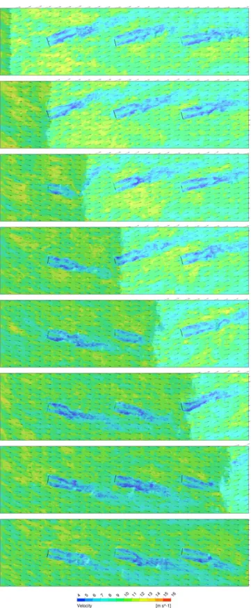
Figure 6 shows velocity contours taken in the xy-plane for the gust event moving through the computational do-main. The first plot shows the effect of the mass-correction profile, with the high velocity region in the gust structure accompanied by a reduced velocity above. The third contour plot shows the propagation of the gust through the wake of the first turbine. Some vertical deflection of the gust is also observed. The subsequent sequence shows further decay of the gust structure along the domain.
C. Wind Shift in an ABL
In order to minimise the effects of us on the change in mass-flow rate, an initial wind angle of θ0 = −15◦ was
selected, with a direction change of θs = 30◦. The wind direction is then given byθ=θ0+θs. An initial wind turbine
yaw angle,γ0=−15was set to correspond with the initial
wind direction.
Figure 7 illustrates the time history of wind direction through the domain indicating that the model described is operating as expected. The time-delays equal to the monitor point distance from the inlet are shown as expected. The effect of turbulence in the domain is also evident as the initial rapid change in direction decays as the front passes successive turbine locations.
D. Wind Shift Propagating through a Wind Farm
The same wind shift structure was introduced to a simula-tion including the wind turbine models. Figure 8 shows the time history of turbine yaw errorγerr, and turbine yaw angle γ. The arrival of the shift front is indicated by the peaks in yaw error at times proportional to the turbine location in the domain. The peaks in yaw error are accompanied by changes in the turbine yaw angle by the yaw controller.
The variation of turbine power with time is shown in Figure 9, with reductions in output evident times correspond-ing to large yaw errors. Power output is also observed to fluctuate significantly following the transit of the shift front, illustrating the disturbed flow created by the wind shift.
Fig. 6. Contour plots of velocity magnitude shown in anxyplane from the positivez direction, for a gust event propagating through the turbine array. The gust is illustrated by the yellow and red region of fluid moving from left to right. The time between plots is∆τs= 3. The turbine rotors are shown as black vertical lines.
the turbine wakes with the initial wind direction angle and corresponding turbine yaw angles. The shearing effect of the
-30 -20 -10 0 10 20 30
-10 -5 0 5 10 15 20 25 30
θ
[
°
]
τs = tUref/D
Fig. 7. A time-series of the wind direction at various locations in the domain starting with the inlet (dashed line), followed by the three turbine hub locations in black, grey and light grey. The plot shows mixing of the shift front by turbulence as it propagates through the domain.
-30 -20 -10 0 10 20 30 40
-10 -5 0 5 10 15 20 25 30
γerr
,
γ
[
°
]
τs = tUref/D
Fig. 8. A time-series of nacelle yaw error γerr (solid) and nacelle yaw angleγ(dashed) for the the first through third turbine hub locations indicated in black, grey and light grey respectively.
0.4 0.5 0.6 0.7 0.8 0.9 1
-10 -5 0 5 10 15 20 25 30
P/P
ref
τs = tUref/D
Fig. 9. A time-series of wind turbine power output relative to rated power for the the first through third turbine hub locations indicated in black, grey and light grey respectively.
it is convected through the domain. Yaw actuation is observed at all turbine locations.
Fig. 10. Contour plots of velocity shown in thexz-plane for a wind shift event propagating through the turbine array. The shift front is illustrated by the shaded region of fluid moving from left to right. Velocity vectors have also been sampled across the plane to illustrate the wind direction.
∆τs= 4. The turbine rotors are shown as black lines.
V. CONCLUSIONS
A methodology for implementing a gust model and wind shift model in a CFD flow domain has been described.
The gust model has been applied to the flow through an array of wind turbines, with the gust structure observed to propagate through the array with a decay in magnitude. The gust structure is transported by the mean convection velocity in the boundary layer. A wind direction shift has also been applied to an array of wind turbines implemented with baseline yaw controllers. The expected reductions in power due to yaw error were observed. The shift front is also observed to propagate with the free-stream wind speed.
ACKNOWLEDGEMENTS
The authors would like to acknowledge the funding of a University of Auckland Doctoral Scholarship. The contribu-tions to the CFD code by S. Armfield from The University of Sydney are greatly appreciated. New Zealand’s national computing facilities are provided by the NZ eScience In-frastructure (NeSI). The authors wish to acknowledge the contribution of the NeSI facilities to the results of this research. URL http://www.nesi.org.nz.
REFERENCES
[1] D. J. Laino and A. C. Hansen, “User’s guide to the wind turbine aerodynamics computer software AeroDyn,” NREL, Tech. Rep., 2002. [2] E. Hau,Wind Turbines: Fundamentals, Technologies, Applications,
Economics. Oxford: Springer, 2006.
[3] BS EN61400-1:2005, Wind turbines Part 1: Design requirements, 2006.
[4] R. C. Storey, S. E. Norris, and J. E. Cater, “An actuator sector method for efficient transient wind turbine simulation,”Accepted for publication in Wind Energy, 2013.
[5] S. W. Armfield, S. E. Norris, P. Morgan, and R. Street, “A parallel non-staggered Navier-Stokes solver implemented on a workstation cluster,” inComputational Fluid Dynamics 2002: ICCFD2, 2003, pp. 30–45. [6] S. E. Norris, “A parallel Navier–Stokes solver for natural convection
and free surface flow,” Ph.D. dissertation, University of Sydney, 2000. [7] S. W. Armfield and R. Street, “An analysis and comparison of the time accuracy of fractional-step methods for the Navier-Stokes equations on staggered grids,”International Journal for Numerical Methods in Fluids, vol. 38, pp. 255–282, 2002.
[8] C. M. Rhie and W. L. Chow, “Numerical study of the turbulent flow past an airfoil with trailing edge separation,”AIAA Journal, vol. 21, no. 11, pp. 1525–1532, 1983.
[9] J. Smagorinsky, “General circulation experiments with the primitive equations,”Monthly Weather Review, vol. 91, no. 3, pp. 99–164, 1963. [10] P. Mason and D.J.Thomson, “Stochastic backscatter in large-eddy simulations of boundary layers,”J. Fluid Mech., vol. 242, pp. 51–78, 1992.
[11] P. Mason and N. Callen, “On the magnitude of the subgrid-scale eddy coefficient in large-eddy simulations of turbulent channel flow,” J. Fluid Mech., vol. 162, pp. 439–462, 1986.
[12] M. Spencer, K. A. Stol, and J. E. Cater, “Predictive yaw control of a 5mw wind turbine,” inProceedings of the 31th Wind Energy Symposium. AIAA, 2012.
[13] J. Jonkman, S. Butterfield, W. Musial, and G. Scott, “Definition of a 5-MW reference wind turbine for offshore system development,” National Renewable Energy Laboratory, Tech. Rep., 2009.
[14] H. J. T. Kooijmann, C. Lindburg, D. Winkelaar, and E. L. van der Hooft, “Dowec 6MW pre-design: Aero-elastic modelling of the dowec 6MW pre-design in phatas,” Energy Research Center of the Nether-lands (ECN), Tech. Rep., 2003.
[15] J. M. Jonkman and M. L. B. Jr., “FAST User’s Guide,” National Renewable Energy Laboratory, Tech. Rep., 2005.
[16] R. C. Storey, S. E. Norris, K. A. Stol, and J. E. Cater, “Large eddy simulation of dynamically controlled wind turbines in an offshore environment,” Wind Energy, 2012. [Online]. Available: http://dx.doi.org/10.1002/we.1525