ISSN 0101-8205 www.scielo.br/cam
Numerical resolution of cone-constrained
eigenvalue problems
A. PINTO DA COSTA1 and ALBERTO SEEGER2
1Universidade Técnica de Lisboa, Instituto Superior Técnico
Departamento de Engenharia Civil e Arquitectura and ICIST Avenida Rovisco Pais, 1049-001 Lisboa, Portugal
2University of Avignon, Department of Mathematics, 33 rue Louis Pasteur
84000 Avignon, France
E-mails: [email protected] / [email protected]
Abstract. Given a convex coneK and matricesAand B, one wishes to find a scalarλand a nonzero vectorxsatisfying the complementarity system
K ∋x⊥(Ax−λBx)∈K+.
This problem arises in mechanics and in other areas of applied mathematics. Two numerical techniques for solving such kind of cone-constrained eigenvalue problem are discussed, namely, the Power Iteration Method and the Scaling and Projection Algorithm.
Mathematical subject classification: 65F15, 90C33.
Key words: complementarity condition, generalized eigenvalue problem, power iteration method, scaling and projection algorithm.
1 Introduction
The Euclidean spaceRn is equipped with the inner producthy,xi = yTx and
the associated normk ∙ k. The dimensionnis greater than or equal to 2. Orthog-onality with respect toh∙,∙iis indicated by means of the symbol⊥.
out this work, one assumes that:
K is a pointed closed convex cone inRn,
AandBare real matrices of sizen×n,
hx,Bxi>0 for all x ∈K\{0}. (1)
We are interested in solving numerically the following cone-constrained
generalized eigenvalue problem. As usual,K+indicates the positive dual cone
ofK.
Problem 1.
Findλ∈Rand a nonzero vectorx ∈Rnsuch that
K ∋x ⊥(Ax−λBx)∈ K+.
Problem 1 arises in mechanics [9, 10] and in various areas of applied mathe-matics [4, 5, 6, 12, 13]. The specific meanings ofAandBdepend on the context. It it important to underline that, in the present work, the matrices Aand Bare not necessarily symmetric.
An interesting particular case of Problem 1 is the so-called Pareto eigenvalue problem, whose precise formulation reads as follows.
Problem 2.
Findλ∈Rand a nonzero vectorx ∈Rnsuch that
Rn+∋x ⊥(Ax−λx)∈R
n
+.
2 Numerical experience with the SPA
All computational tests are carried out for the particular choice B = In, but
the formulation of the SPA is given for a general matrix B as in (1). The SPA
is an iterative method designed for solving Problem 1 written in the following equivalent form:
Problem 3.
Findλ∈Rand vectorsx,y ∈Rnsuch that
(A−λB)x = y
K ∋ x ⊥y ∈ K+
φ(x)=1. (2)
The normalization condition (2) prevents x from being equal to 0. Adding
such condition does not change the solution set of the original cone-constrained
generalized eigenvalue problem. As example of functionφ, one may think of
φ(x) = kxk,
φ(x) = phx,Bxi,
φ(x) = he,xi with e ∈int(K+), (3)
but other options are also possible. Our favorite choice is the linear function (3) because in such a case the set
Kφ =
x ∈ K : φ (x)=1
is not just compact, but also convex. In the parlance of the theory of convex cones, the set Kφ corresponds to a “base” ofK. Unless explicitly stated other-wise, we assume that the choice (3) is in force.
The SPA generates a sequence{xt}
t≥0inKφ, a sequence{λt}t≥0of real
num-bers, and a sequence{yt}t≥0of vectors inRn. The detailed description of the
algorithm is as follows:
• Initialization: Fix a positive scaling factor s. Pick u ∈ K\{0} and let
• Iteration: One has a current pointxt inKφ. Compute the Rayleigh-Ritz ratio
λt = hxt,Axti/hxt,Bxti,
the vectoryt = Axt −λ
tBxt,and the projection
vt =5K[xt−syt].
The projection vt is necessarily in K\{0}. Proceed now to a φ -normal-ization:
xt+1=vt/φ(vt) .
One could perfectly well consider a scaling factor that is updated at each iteration, but in this section we stick to the case of a fixed scaling factor. The case of a variable scaling factor will be commented in Section 4. The next convergence result is taken from [11].
Theorem 1. If{xt}
t≥0converges to a certain vectorx, thenˉ
(a) {λt}t≥0converges toλˉ = h ˉx,Axˉi/h ˉx,Bxi.ˉ
(b) {yt}
t≥0converges toyˉ = Axˉ − ˉλBx.ˉ
(c) (xˉ,λ,ˉ yˉ)solves Problem3.
2.1 Applying the SPA to the Pareto eigenvalue problem
The Pareto eigenvalue problem already exhibits many of the mathematical dif-ficulties arising in the context of a general convex coneK. While dealing with the Pareto coneRn
+one chooses
φ(x)=x1+x2+. . .+xn (4)
as normalizing function. This corresponds to the linear choice (3) with e =
(1,1, . . . ,1)T belonging to the interior ofRn+.
A few words on terminology are appropriate at this point in time. One usually refers to
σpareto(A)=
as the Pareto spectrum (or set of Pareto eigenvalues) of A. The mapσpareto: Mn →2Rhas some similarities with the classical spectral map, but the differ-ences are even more numerous. It deserves to be stressed that
πn = max A∈Mn
cardσpareto(A)
is finite, but grows exponentially with respect to the dimensionnof the underly-ing Euclidean space. Thus, a matrix of a relatively small size could have a very large number of Pareto eigenvalues. In view of this observation, it is simply not reasonable to try to compute all the elements ofσpareto(A). A more realistic goal
is finding just one or a bunch of them.
2.1.1 Testing on a2×2matrix with3Pareto eigenvalues
We start by considering the 2×2 matrix
A=
"
8 −1
3 4
#
(5)
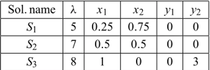
whose Pareto spectrum is displayed in Table 1. For ease of visualization, the Pareto eigenvalues are arranged in increasing order. The corresponding solutions are named starting fromS1up toS3.
Sol. name λ x1 x2 y1 y2
S1 5 0.25 0.75 0 0
S2 7 0.5 0.5 0 0
S3 8 1 0 0 3
Table 1 – Solution set of the Pareto eigenproblem associated with matrix (5).
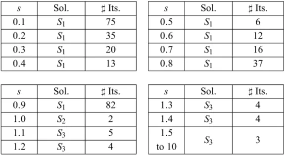
For this small size matrix, the SPA was able to detect all the solutions. Table 2
shows which solution was detected as function of a scaling parameters varying
in steps of 0.1 units.
s Sol. ♯Its. s Sol. ♯Its.
0.1 S1 75 0.5 S1 6
0.2 S1 35 0.6 S1 12
0.3 S1 20 0.7 S1 16
0.4 S1 13 0.8 S1 37
s Sol. ♯Its. s Sol. ♯Its.
0.9 S1 82 1.3 S3 4
1.0 S2 2 1.4 S3 4
1.1 S3 5 1.5
1.2 S3 4 to 10 S3 3
Table 2 – Influence of the scaling factorson the detected solution and on the number of iterations required by the SPA to achieve convergence. The matrixAunder consideration is (5) and the initial point isu=(0,1).
tests show that no changes in the detected solution and in the number of iterations
occur when the parameters is taken beyond a certain threshold value.
Observe that the solutions S1 and S3 were found by several of the values
assumed bys, whereas the solutionS2was detected only with the specific choice s =1. In short, some Pareto eigenvalues are more likely to be found than others.
Remark 1. For a given u, the detected solution and the number of iterations required by the SPA to achieve convergence may be very sensitive with respect
to the parameters. In Table 2 one observes substantial changes while passing
froms=0.9 tos =1.1.
2.1.2 Testing on a3×3matrix with9Pareto eigenvalues
We now test the SPA on the matrix
A=
8 −1 4
3 4 1/2
2 −1/2 6
(6)
Sol.
name λ x1 x2 x3 y1 y2 y3
S1 4.133975 0 1 0.267949 0.071797 0 0
S2 4.602084 0.185257 1 0.092628 0 0 0
S3 5 0.333333 1 0 0 0 0.166667
S4 5.866025 0 0.267949 1 3.732051 0 0
S5 6 0 0 1 4 0.5 0
S6 7 1 1 0 0 0 1.5
S7 8 1 0 0 0 3 2
S8 9.397916 1 0.602084 0.5 0 0 0
S9 10 1 0 0.5 0 3.25 0
Table 3 – Solution set of the Pareto eigenproblem associated with matrix (6).
spectrum of a 3×3 matrix. We know for sure that a 3×3 matrix cannot have
11 or more Pareto eigenvalues. We have not found yet a 3×3 matrix with 10
Pareto eigenvalues and seriously doubt that such a matrix exists.
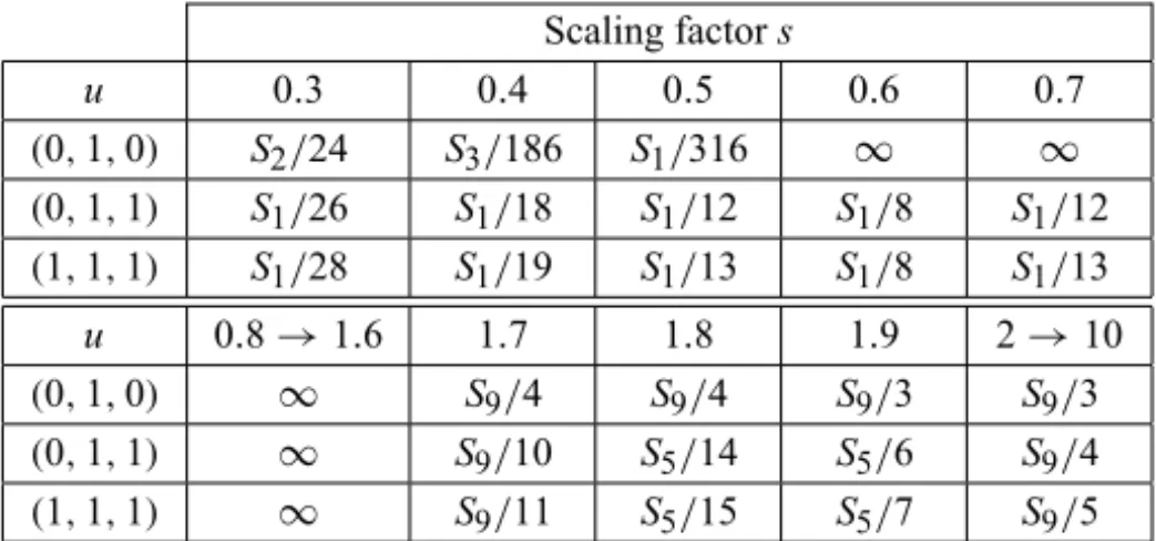
The challenge that (6) offers to the SPA is not the “large” number of Pareto eigenvalues, but the fact that some of them are hard to detect numerically. In Table 4 and in the sequel, the notation Sj/m indicates that the solution Sj was
found withinmiterations and the symbol∞indicates that convergence did not
occur within 2000 iterations. Some of the conclusions that can be drawn from Table 4 are:
i) Given an initial pointu, it is possible to recover several solutions to the
Pareto eigenvalue problem by letting the scaling factors to assume
dif-ferent values. One should not expect however to recover all the solutions (unless of course one changes also the initial point).
ii) Given an initial pointu, there are values ofsfor which the SPA does not converge. It is very difficult to identify the convergence region
S(u)≡values ofs for which SPA converges when initialized atu
Scaling factors
u 0.3 0.4 0.5 0.6 0.7
(0,1,0) S2/24 S3/186 S1/316 ∞ ∞ (0,1,1) S1/26 S1/18 S1/12 S1/8 S1/12 (1,1,1) S1/28 S1/19 S1/13 S1/8 S1/13
u 0.8→1.6 1.7 1.8 1.9 2→10
(0,1,0) ∞ S9/4 S9/4 S9/3 S9/3 (0,1,1) ∞ S9/10 S5/14 S5/6 S9/4 (1,1,1) ∞ S9/11 S5/15 S5/7 S9/5
Table 4 – Influence of the initial pointuand the scaling factorson the detected solution and on the number of iterations required by the SPA to achieve convergence. The matrix under consideration is (6).
2.1.3 Testing on random matrices and random initial points
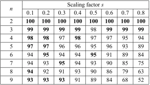
Table 5 has been produced as follows. For each dimensionn ∈ {2,3, . . . ,9}, one generates a collection of 1000 stochastically independent random matrices with uniform distribution on the hypercube[−1,1]n×n. For each one of these 1000 random matrices, one generates a collection of 100 stochastically independent random initial vectors with uniform distribution on the hypercube[0,1]n. One
applies the SPA to each one of the 105 =1000×100 random pairs(A,u)and
counts the number of times in which convergence occurs within 2000 iterations. As one can see from Table 5, the best performances of the SPA are obtained when the scaling factorslies in the interval[0.1,0.4]. Whens is taken in such range, the percentages of convergence are all above 90 per cent. This good new speaks favorably of the SPA. The same experience as in Table 5 is carried out for
n ∈ {10,20,30,100}, but with a different set of values for the scaling factors. Table 6 displays the obtained results. One sees that the overall performance of
the SPA diminishes as the dimensionngets larger. Forn =100 the best score
of convergence is 78%. This is still acceptable.
Table 7 reports on the casen ∈ {200,300,400,500,1000}. In this range of dimensions, the performance of the SPA is a bit less satisfactory. For instance,
n Scaling factors
0.1 0.2 0.3 0.4 0.5 0.6 0.7 0.8
2 100 100 100 100 100 100 100 100
3 99 99 99 99 98 99 99 99
4 98 98 97 98 97 97 95 94
5 97 97 96 96 95 96 93 89
6 94 95 94 94 95 91 89 84
7 94 93 95 94 93 90 85 75
8 94 92 91 93 90 86 79 63
9 93 93 93 91 89 84 68 52
Table 5 – SPA applied to a sample of 105random pairs(A,u). The figures on the table
refer to percentages of convergence. The best performances for eachn ∈ {2,3, . . . ,9} are indicated with a bold font.
n Scaling factors
0.04 0.05 0.06 0.07 0.08 0.09 0.1 0.2
10 33 51 70 85 90 93 91 91
20 44 66 80 86 87 89 88 87
30 53 72 85 83 85 87 86 80
100 75 76 77 76 78 76 78 64
Table 6 – SPA applied to a sample of 105 random pairs (A,u). The figures on the table refer to percentages of convergence. The best performances for each
n∈ {10,20,30,100}are indicated with a bold font.
n Scaling factors
0.03 0.04 0.05 0.06 0.07 0.08 0.09 0.1
200 66 72 70 71 72 72 69 69
300 65 70 69 67 71 65 63 64
400 66 66 65 67 62 62 60 54
500 64 67 63 63 64 61 57 50
1000 58 62 60 54 45 × × ×
Table 7 – SPA applied to a sample of 105 random pairs (A,u). The figures on the table refer to percentages of convergence. The best performances for each
2.2 Applying the SPA to a circular eigenvalue problem
A circular eigenvalue problem is a prototype of eigenvalue problem with con-straints described by a nonpolyhedral cone:
Problem 4.
Findλ∈Rand a nonzero vectorx ∈Rnsuch that
Lθ ∋x ⊥(Ax−λx)∈L+θ.
(7)
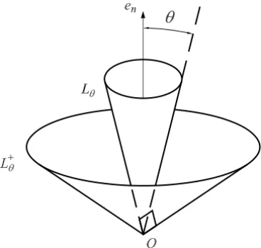
Here,Lθstands for then-dimensional circular cone whose half-aperture angle isθ ∈]0, π/2[, and whose revolution axis is the ray generated by the canonical vectoren=(0, . . . ,0,1)T. In short,
Lθ =
x ∈Rn:(cosθ )kxk ≤xn . (8)
A circular eigenvalue problem differs substantially from a Pareto eigenvalue problem, the main difference being that a circular spectrum
σθ(A)=
λ∈R: (x, λ)solves Problem 4
does not need to be finite. As shown in [16], the setσθ(A)could perfectly well contain one or more intervals of positive length.
As seen in Figure 1, the dual cone of Lθ is again a circular cone. In fact, as reported in [3], one has the general relation L+θ = L(π/2)−θ. The projection of z ∈RnontoL
θ can be evaluated by using the explicit formula
5Lθ[z] =
z if z ∈ Lθ
0 if z ∈ −L+θ
v if z ∈Rn\(Lθ ∪ −L+θ)
with
vi = zi − p
kzk2−z2
n−zntanθ 1+[tanθ]2
zi p
kzk2−z2
n
∀i ∈ {1, . . . ,n−1},
vn = zn+ p
kzk2−z2
n−zntanθ
1+[tanθ]2 tanθ.
The above expression ofvcan be found in [1] or obtained simply by working
out the Karush-Kuhn-Tucker optimality conditions for the convex minimization problem
minimize kx−zk2
x ∈Rns.t.(cosθ )kxk ≤xn.
For dealing with the circular eigenvalue problem, one uses
φ (x)=xn (9)
as normalization function. This corresponds to the linear choice (3) with vector
e=en. Note thatenbelongs to the interior ofL+θ.
A convex cone whose half-aperture angle is 90 degrees is no longer pointed, so the SPA implemented with the linear normalizing function (9) could run into numerical troubles ifθ increases beyond a certain threshold.
We are interested in examining the performance of the SPA as function of the
half-aperture angleθ of the circular cone. The numerical experiment reported
in Table 8 concerns a sample of 105random pairs(A,u)generated in the same way as in Tables 5, 6, and 7. The SPA is tested with three different values ofs
θ Scaling factors θ Scaling factors θ Scaling factors
0.05 0.1 1 0.05 0.1 1 0.05 0.1 1
5 100 100 100 5 100 100 100 5 100 100 100
15 100 100 100 15 100 100 100 15 100 100 100
25 99 99 99 25 100 100 100 25 100 100 100
35 94 99 96 35 100 100 63 35 100 100 53
45 88 97 93 45 100 100 1 45 100 100 0
55 78 93 86 55 98 99 0 55 100 100 0
65 69 89 83 65 91 91 0 65 93 95 0
75 63 83 78 75 74 73 0 75 72 74 0
85 57 80 74 85 40 54 0 85 39 50 0
Table 8 – SPA applied to a sample of 105random pairs(A,u). One considers the cases n =3 (left),n =50 (middle), andn =100 (right). The figures on the tables refer to percentages of convergence.
i) For each tested scaling factor s and dimension n, one observes that the
rate of success of the SPA decreases as the half-aperture angle increases. The best results are obtained for circular cones with moderate half-aperture angle. As predicted by common sense, dealing with circular cones with half-aperture angle near 90 degrees is problematic.
ii) As we already saw in previous numerical experiences, a right choice of scaling factor is crucial for obtaining a good performance of the SPA. As a general rule, when dealing with large dimensional problems one
should reduce the size of the parameter s. As one can see in the
mid-dle table and in the right table, the choice s = 1 is appropriate only if the half-aperture angle does not exceed 25 degrees. Beyond this angular threshold, the performance of the SPA deteriorates very quickly. By con-trast, if one uses a smaller scaling factor, says =0.1, then the SPA works perfectly well in a wider range of half-aperture angles.
3 Theory and numerical experience with the PIM
ann×nreal matrix Mwith real eigenvaluesλ1, . . . , λnsuch that |λ1|>|λ2|> . . . >|λn|.
The classical power iteration method consists in generating a sequence{xt}t≥0
by selecting an initial pointx0and applying the recursive formula xt+1= M x
t
φ (M xt), (10)
whereφ is typically the Euclidean normk ∙ kor a certain linear function. One
expects the sequence{xt}
t≥0to converge to an eigenvectoru1associated to the
eigenvalueλ1. See, for instance, Section 13.4 in Schatzman’s book [14] for a
pre-cise formulation of the convergence result. The limitu1satisfies necessarily the
normalization conditionφ (u1)=1. The eigenvalueλ1is obtained by using
ei-ther the relationλ1=φ (Mu1)or the Rayleigh-Ritz ratioλ1= hu1,Au1i/ku1k2. Remark 2. If one wishes to find a different eigenvalue, then one chooses a
convenient shifting parameterβ ∈ Rand applies the iteration scheme (10) to
the shifted matrixM −βIn. By the way, the so-called inverse power iteration method consists in applying (10) to the inverse of the matrixM−βIn.
It is not difficult to adjust the power iteration method to the case of a generalized eigenvalue problem involving a pair(A,B)of matrices. However, incorporating a coneK into the picture is a matter that requires a more careful thinking. For the sake of clarity in the discussion, we leave aside the matrixBand concentrate
onK. The problem at hand reads as follows.
Problem 5.
Findλ∈Rand a nonzero vectorx ∈Rnsuch that
K ∋x ⊥(Ax −λx)∈ K+.
In principle, the usual spectrum of Ahas very little to do with
σK(A)=
the latter set being called theK- spectrum (or set ofK- eigenvalues) ofA. How-ever, regardless of the choice ofK, one always has the inclusion
σK(A)⊂
λmin Asym
, λmax Asym
, (11)
with λmin(Asym) and λmax(Asym) denoting, respectively, the smallest and the
largest eigenvalue of the symmetric part
Asym=
A+AT 2
of the matrix A. The computation of the extremal eigenvalues of a symmetric
matrix presents no difficulty.
Lemma 1. Consider anyβ ∈Rsuch that
β > λmax Asym
. (12)
Then, the following conditions are equivalent:
(a) x is a K - eigenvector of A.
(b) x and5K[βx−Ax]are nonzero vectors pointing in the same direction.
Proof. For allλ∈Randx ∈Rn, one has the general identity
βx −Ax =(β−λ)x−(Ax −λx).
This relation is at the core of the proof. Let x be a K- eigenvector of A and
letλbe the associatedK- eigenvalue. In particular,x is a nonzero vector in K. Furthermore, the combination of (11) and (12) shows thatγ =β−λis a positive scalar. By applying Moreau’s theorem [8] to the orthogonal decomposition
βx−Ax = γ x
|{z}
∈K
−Ax−λx
| {z }
∈K+
,
one obtains
γx =5K
This confirms that x and 5K[βx − Ax] are nonzero vectors pointing in the
same direction. Conversely, suppose that x 6= 0 and that (13) holds for some
positive scalarγ. Then, one can draw the following conclusions. Firstly,x ∈ K
because γx ∈ K andγ > 0. Secondly, in view of Moreau’s theorem, the
equality (13) yields
γx −(βx−Ax) ∈ K+,
hγx, γx−(βx −Ax)i = 0.
We have proven in this way thatxis a nonzero vector satisfying the
complemen-tarity system
K ∋x ⊥(Ax−(β−γ )x)∈ K+.
In other words, x is a K- eigenvector of A andλ = β −γ is the associated
K- eigenvalue.
Condition (b) in Lemma 1 provides the inspiration for the formulation of the PIM in the context of a cone-constrained eigenvalue problem. The detailed description of this algorithm is as follows:
• Initialization: Select a shifting parameter β as in (12). Pick a nonzero vectoru ∈ K and letx0=u/φ(u).
• Iteration: One has a current pointxt inKφ. Compute first the projection
vt =5K
βxt−Axt, (14)
and then theφ-normalized vector
xt+1=vt/φ (vt). (15)
As was the case with the SPA, a sequence generated by the PIM remains in the compact setKφ. The emphasis of the PIM is the computation ofK- eigenvectors. If one wishes, at each iteration one can also evaluate the Rayleigh-Ritz ratio
Theorem 2. Let{xt}t≥0be generated by the PIM.
(a) The general term xt is well defined, i.e., the projection vt is different from0.
(b) If{xt}t≥0converges to a certainx, thenˉ x is a K - eigenvector of A.ˉ
(c) The K -eigenvalue of A associated tox is given byˉ
ˉ
λ = h ˉx,Axiˉ /k ˉxk2 = β−φ (5K[βxˉ−Axˉ]). (16)
Proof. Suppose, on the contrary, thatvt = 0 at some iterationt. From the usual characterization of a projection, one has
hβxt −Axt, wi ≤0 ∀w∈ K.
In particular,hβxt −Axt,xti ≤0.Sincext 6=0, one obtains
β ≤ hx t,Axti
kxtk2 ≤λmax Asym
,
a contradiction with assumption (12). This takes care of (a). Suppose now that
{xt}
t≥0 converges to xˉ. By passing to the limit in (14) one sees that {vt}t≥0
converges to
ˉ
v=5K[βxˉ −Ax]ˉ .
As done before with each termvt, one can also prove thatvˉ is different from 0. By passing now to the limit in (15), one gets
ˉ
x = ˉv/φ (v).ˉ
Sinceγˉ = φ (v)ˉ is a positive scalar, the nonzero vectorsxˉ andvˉ are pointing
in the same direction. In view of Lemma 1, one concludes that xˉ is a K
-eigenvector of A. The first equality in (16) is obvious, while the second one
is implicit in the proof of Lemma 1.
The inequality (12) has been helpful at several stages. Lemma 1 and The-orem 2 remain true if one works under the weaker assumption
β > sup x∈K
kxk=1
but the evaluation of the above supremum could be a bothersome task. From a purely theoretical point of view, one could even work under the assumption
β > sup λ∈σK(A)
λ. (17)
In practice, it makes no sense relying on (17) because σK(A) is unknown
a priori.
3.1 Applying the PIM to the Pareto eigenvalue problem
3.1.1 Testing on a small size matrix
We start by testing the PIM on the matrix (6). Recall that (6) is a nonsymmetric 3×3 matrix with 9 Pareto eigenvalues. All of them are positive and the largest
one isλ=10. A straightforward computation shows that
Asym=
8 1 3
1 4 0
3 0 6
, λmax Asym
=10.2682.
The symbol∞in Table 9 means, as usual, that convergence does not occur
within 2000 iterations. Observe that number of iterations required by the PIM
to achieve convergence increases asβ goes further and further away from the
threshold value (17). So, it is not a good idea to takeβ excessively large.
Shifting parameterβ
u 5 6 7 8 9 10 11 20 50
(0,1,0) E ∞ ∞ S2/22 S2/9 S2/10 S2/14 S2/47 S2/143 (0,1,1) E S1/8 S1/21 S1/31 S1/41 S1/50 S1/60 S1/140 S1/391
(1,1,1) E E E S1/32 S1/42 S1/51 S1/61 S1/143 S1/397
Table 9 – Influence of the initial pointuand the parameterβ on the detected solution and on the number of iterations required by the PIM to achieve convergence. The matrix under consideration is (6).
On the other hand, the symbol E in Table 9 indicates that an error occurs
while performing the first iteration of the PIM. To be more precise, the PIM
situation does not contradict the statement (a) of Theorem 2. What happens is
simply that the value ofβ under consideration does not satisfy the assumption
(12), not even the weaker condition (17). In connection with this issue, it is
worthwhile mentioning that if one uses a parameter β smaller than the
right-hand side of (17), then the PIM may still work in the sense that each projection
vt may be different from 0 and {xt} may converge to a K- eigenvector of A.
Logically speaking, (17) is a sufficient condition for the PIM to work properly, but such condition is not necessary.
In Table 10 one applies the PIM to the matrix (6), but one considers a sample of 108random initial points. The question that is being addressed is the following
one: to which Pareto eigenvalue of (6) is the PIM most likely to converge?
β Obtained solution % of
S1 S2 S3 S4 S5 S6 S7 S8 S9 None success
10 48.6 0 11.3 0 26.4 0 13.7 0 0 0 100.0
15 52.4 0 10.6 0 22.6 0 14.4 0 0 0 100.0
20 47.1 0 10.4 0 21.8 0 14.6 0 0 6.1 93.9 25 47.2 0 10.4 0 21.4 0 14.6 0 0 6.5 93.5
Table 10 – PIM applied to the matrix (6). The figures on the table refer to percentages of convergence to each particular solution. A sample of 108random initial points is being considered.
3.1.2 Testing on random matrices and random initial points
The same kind of numerical experiment as in Section 2.1.3 is now carried out with the PIM. To avoid excessive repetitions, we consider only the case of a dimensionnranging over{3,6,12}.
Since one works with a sample of random pairs(A,u), it is not entirely clear
how to choose the parameterβin order to optimize the performance of the PIM.
In Table 11 we explore what happens with the choices
βk =λmax Asym
+(k/2)−1 with k =1,2,3,4. (18)
Note thatβ1is smaller thanλmax Asym
the distribution of the random variableλmax Asym
whenn ∈ {3,6,12}.
n Shifting parameterβ
β1 β2 β3 β4
3 81 99 98 98
6 92 94 95 95
12 89 91 89 91
Table 11 – PIM applied to a sample of 105random pairs(A,u). The best performances for each dimensionn∈ {3,6,12}are indicated with a bold font.
The figures on Table 11 refer to percentages of success. The word “success” means, of course, that the PIM has worked properly, failure corresponding to a case of lack of convergence or to the obtention of a projection equal to 0. As one
can see, the percentages of success of the PIM do not change too much whenβ
ranges over (18).
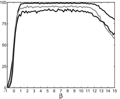
In Figure 2 we enlarge the field of values taken by the parameterβ. The idea is identifying the largest interval over whichβ leads to a favorable and stable rate of success.
-10 0 1 2 3 4 5 6 7 8 9 10 11 12 13 14 15
25 50 75 100
β
One observes a very interesting plateau phenomenon: for each dimensionn, there is a corresponding range[βnlower, βnupper]of values forβ in which the PIM performs at its top level. The height of each plateau depends on the dimension: the height decreases asnincreases. Note also that the interval[βnlower, βnupper]is almost identical for the three tested values ofn.
4 SPAversusPIM
From a conceptual point of view, the SPA and the PIM are different methods. However, they share in common at least two important steps: a projection onto
the coneK and aφ-normalization procedure.
Are the SPA and the PIM two different algorithms after all? The answer is yes if the scaling factorsand the shifting parameterβare not allowed to change from one iteration to the next. If one is more flexible and considers instead a sequence{st}t≥0of scaling factors and a sequence{βt}t≥0of shifting parameters,
then one can reformulate the SPA as a PIM, and viceversa.
Proposition 1. Let B =In. The following statements are true:
(a) Implementing the t-th iteration of the PIM with βt > hxt,Axti/kxtk2 produces the same outcome as implementing the t-th iteration of the SPA with
st =
βt −
hxt,Axti kxtk2
−1
. (19)
(b) Conversely, implementing the t-th iteration of the SPA with st > 0 pro-duces the same outcome as implementing the t-th iteration of the PIM with
βt = 1
st +hx
t,Axti
kxtk2 . (20)
Proof. The projection map5K and the normalizing functionφare both posi-tively homogeneous. Hence,φ-normalizing the projected vector5K[xt−styt] produces the same result asφ-normalizing the projected vector5K[(1/st)xt − yt]. It suffices then to observe that
(1/st)xt −yt =βtxt −Axt ⇐⇒(1/st)xt −(Axt−λtxt)=βtxt−Axt
with λt = hxt,Axti/kxtk2. Of course, one rewrites the equality (21) in the
form (19) for proving part (a), and in the form (20) for proving part (b).
4.1 Numerical experience with a sequence{st}t≥0
We have tested again the SPA on random matrices and random initial points, but this time we have used a variable scaling factorst. The attention is focused
on dimensions not exceeding n = 30. Inspired by the relation (19) and the
experimental data reported in Figure 2, we choose a scaling factorst obeying to the feedback rule
st =
β−hx t,Axti kxtk2
−1
with β =6. (22)
The word “feedback” is used here to indicate that st is updated by taking in
account the current valuext of the state vector x.
Table 12 reports on the outcome of this experiment. The most important lesson of this experiment is the following one: the SPA implemented with the feedback rule performs equally well as the SPA implemented with the constant scaling factorsthat is optimal for the prescribed dimension. For instance, when
n = 9, the feedback rule leads to a rate of success of 93%, a percentage that
matches the rate of success of the SPA implemented with the optimal choice
s =0.1 (cf. Table 5).
n 3 6 9 12 15 18 21 24 27 30
% 99 95 93 90 89 89 87 88 85 86
Table 12 – For eachn ∈ {3,6,9, . . . ,30}, the SPA was applied to a sample of 105 random pairs(A,u). The variable scaling factor used was (22). Figures correspond to percentages of convergence.
5 By way of conclusion
Our main comments on the SPA and the PIM are as follows:
1. The SPA generates a bounded sequence{(xt, λ
t,yt)}t≥0 that depends on
2. The SPA does not aim at finding all the solutions to Problem 3. This is not just because the number of solutions could be very large, but also be-cause some solutions could be extremely hard to be detected. It happens in practice that some solutions are hard to be found even if the SPA is initial-ized at a convenient initial point. The existence of such “rare” solutions is somewhat intrinsic to the nature of the cone-constrained eigenvalue prob-lem. An interesting open question is understanding why some solutions are so hard to be detected and others are not. An appropriate theoretical analysis remains to be done.
3. The SPA was extensively tested in the Paretian case. One of the main conclusions of Section 2.1 is that the scaling factors >0 must be chosen with care if one wishes the SPA to produce a convergent sequence. Exten-sive numerical experimentation has been carried out for Pareto eigenvalue
problems with random data. Specifically, the entries of the matrix Aand
the entries of the initial vectoruwere considered as independent random variables uniformly distributed over the interval [−1,1]. For each di-mensionn, there is a convenient range of values for the scaling factors.
A good choice ofsis one for which the SPA converges in a vast majority
of cases, see Tables 5, 6, and 7.
4. The PIM has the advantage of relying on a parameter β that is not too
sensitive with respect to dimensionality. Thanks to the plateau phenom-enon described in Section 3.1.2, there is no need of putting too much effort in selecting the shifting parameterβ. One just needs to make sure thatβ lies in a certain range that is easily identifiable.
We end this work by mentioning an open alternative. Observe that Problem 3 is about finding a triplet(x, λ,y)that lies in the closed convex coneQ = K ×
R×K+,and that solves the system of nonlinear equations
Ax−λBx−y = 0,
hx,yi = 0,
In principle, one could apply any method for solving systems of nonlinear equations on closed convex cones. Do such methods exist in the literature? Are they efficient? These questions open the way to a broad discussion that deserves a detailed treatment in a separate publication.
A natural idea that comes to mind is finding a global minimum over Qof the
residual term
f(x, λ,y)=μ1kAx−λBx−yk2+μ2hx,yi2+ [φ(x)−1]2,
whereμi are positive scalars interpreted as weight coefficients. For instance, Friedlander et al., [2] use a residual minimization technique for solving a so-called horizontal linear complementarity problem. However, in our particular context, one should not be too optimistic about residual minimization. Indeed, this technique may produce a local minimum that is not a global one.
Last but not the least, our original motivation was solving a very specific cone-constrained eigenvalue problem arising in mechanics (namely, detecting directional instabilities in elastic systems with frictional contact). The problem at hand is highly structured and will be treated in full extent in a forthcoming work. However, we want to mention here some features that could be of interest for non-specialists:
– Firstly, the cone defining the constraints is a Cartesian product K =
K1×. . .×KN of a large number of closed convex cones living in small
dimensional Euclidean spaces. As a consequence of this, the vector
x =(x[1], . . . ,x[N])breaks into N blocks and Problem 1 leads to a
col-lection of subproblems (coupled, in general).
– Secondly, some of the blocks x[r] are unconstrained, i.e., Kr = Rnr.
This means that K is unpointed, a situation that is preferable to avoid.
One way to overcome this difficulty is by applying our algorithms to the constrained subproblems and by treating the unconstrained ones as in clas-sical numerical linear algebra. Of course, all this requires some necessary adjustments.
– Thirdly, the constrained blocksx[r]obey to the unilateral contact law and
on the coefficient of friction. It is also possible to accommodate the more general case of an anisotropic friction law.
Specially structured matrices are not reflected by the random data used in this paper. Our primary concern has been focussing in problems for which the matrix
Ahas no structure whatsoever.
Remark 3. The results presented in Tables 6 and 7 were produced with the IST Cluster, which is a Cluster 1350 computing system from IBM. It has a total of 70 computing nodes each with 2 POWER dual core processors at 2.3 GHz, with 2GB per core. All the nodes are running the AIX 5.3 operating system. The parallel processes were connected using library MPI (Message Passing Interface). The programs developed during this study were writen in FORTRAN.
Acknowledgments. We thank Prof. Moitinho de Almeida (Departmento de Engenharia Civil e Arquitectura, IST, Portugal) for the parallelization of one of the programs developed for this study.
REFERENCES
[1] H.H. Bauschke and S.G. Kruk,Reflection-projection method for convex feasibility problems with an obtuse cone.J. Optim. Theory Appl.,120(2004), 503–531.
[2] A. Friedlander, J.M. Martínez and S.A. Santos,Solution of linear complementarity problems using minimization with simple bounds.J. Global Optim.,6(1995), 253–267.
[3] J.L. Goffin, The relaxation method for solving systems of linear inequalities. Math. Oper. Res.,5(1980), 388–414.
[4] A. Iusem and A. Seeger,On pairs of vectors achieving the maximal angle of a convex cone. Math. Program.,104(2005), 501–523.
[5] J.J. Júdice, M. Raydan, S.S. Rosa and S.A. Santos, On the solution of the symmetric eigenvalue complementarity problem by the spectral projected gradient algorithm. Numer. Algor.,47(2008), 391–407.
[6] J.J. Júdice, I.M. Ribeiro and H.D. Sherali, The eigenvalue complementarity problem. Comput. Optim. Appl.,37(2007), 139–156.
[7] P. Lavilledieu and A. Seeger, Existence de valeurs propres pour les systèmes multivoques: résultats anciens et nouveaux.Annal. Sci. Math. Québec,25(2000), 47–70.
[9] A. Pinto da Costa, I.N. Figueiredo, J.J. Júdice and J.A.C. Martins, A complementarity eigenproblem in the stability of finite dimensional elastic systems with frictional contact. Complementarity: Applications, Algorithms and Extensions, 67–83. Applied Optimization Series, vol. 50. Eds. M. Ferris, O. Mangasarian and J.S. Pang, Kluwer Acad. Publ., Dordrecht. (1999).
[10] A. Pinto da Costa, J.A.C. Martins, I.N. Figueiredo and J.J. Júdice, The directional insta-bility problem in systems with frictional contacts. Comput. Methods Appl. Mech. Engrg.,
193(2004), 357–384.
[11] A. Pinto da Costa and A. Seeger, Cone-constrained eigenvalue problems: theory and algorithms.Comput. Optim. Appl.,43/44(2009), in press.
[12] M. Queiroz, J.J. Júdice and C. Humes, The symmetric eigenvalue complementarity prob-lem.Math. Comp.,73(2004), 1849–1863.
[13] P. Quittner, Spectral analysis of variational inequalities. Comm. Math. Univ. Carolinae,
27(1986), 605–629.
[14] M. Schatzman,Analyse Numérique, Dunod, Paris. (2001).
[15] A. Seeger,Eigenvalue analysis of equilibrium processes defined by linear complementarity conditions.Linear Algebra Appl.,292(1999), 1–14.