ACPD
14, 1559–1615, 2014Free tropospheric NO2from OMI cloud
slicing
S. Choi et al.
Title Page
Abstract Introduction
Conclusions References
Tables Figures
◭ ◮
◭ ◮
Back Close
Full Screen / Esc
Printer-friendly Version
Interactive Discussion
Discussion
P
a
per
|
D
iscussion
P
a
per
|
Discussion
P
a
per
|
Discuss
ion
P
a
per
|
Atmos. Chem. Phys. Discuss., 14, 1559–1615, 2014 www.atmos-chem-phys-discuss.net/14/1559/2014/ doi:10.5194/acpd-14-1559-2014
© Author(s) 2014. CC Attribution 3.0 License.
Atmospheric Chemistry and Physics
Open Access
Discussions
This discussion paper is/has been under review for the journal Atmospheric Chemistry and Physics (ACP). Please refer to the corresponding final paper in ACP if available.
Global free tropospheric NO
2
abundances
derived using a cloud slicing technique
applied to satellite observations from the
Aura Ozone Monitoring Instrument (OMI)
S. Choi1,2, J. Joiner2, Y. Choi3, B. N. Duncan2, and E. Bucsela4
1
Science Systems and Applications Inc., Lanham, MD, USA
2
NASA Goddard Space Flight Center, Greenbelt, MD, USA
3
University of Houston, Houston, TX, USA
4
SRI International, Menlo Park, CA, USA
Received: 6 December 2013 – Accepted: 6 January 2014 – Published: 17 January 2014
Correspondence to: S. Choi (sungyeon.choi@nasa.gov)
ACPD
14, 1559–1615, 2014Free tropospheric NO2from OMI cloud
slicing
S. Choi et al.
Title Page
Abstract Introduction
Conclusions References
Tables Figures
◭ ◮
◭ ◮
Back Close
Full Screen / Esc
Printer-friendly Version
Interactive Discussion
Discussion
P
a
per
|
D
iscussion
P
a
per
|
Discussion
P
a
per
|
Discuss
ion
P
a
per
|
Abstract
We derive free-tropospheric NO2 volume mixing ratios (VMRs) and stratospheric
col-umn amounts of NO2 by applying a cloud slicing technique to data from the Ozone
Monitoring Instrument (OMI) on the Aura satellite. In the cloud-slicing approach, the slope of the above-cloud NO2column vs. the cloud scene pressure is proportional to
5
the NO2 VMR. In this work, we use a sample of nearby OMI pixel data from a single
orbit for the linear fit. The OMI data include cloud scene pressures from the rotational-Raman algorithm and above-cloud NO2vertical column density (VCD) (defined as the
NO2 column from the cloud scene pressure to the top-of-the-atmosphere) from a
dif-ferential optical absorption spectroscopy (DOAS) algorithm. Estimates of stratospheric
10
column NO2 are obtained by extrapolating the linear fits to the tropopause. We
com-pare OMI-derived NO2 VMRs with in situ aircraft profiles measured during the NASA
Intercontinental Chemical Transport Experiment Phase B (INTEX-B) campaign in 2006. The agreement is generally within the estimated uncertainties when appropriate data screening is applied. We then derive a global seasonal climatology of free-tropospheric
15
NO2VMR in cloudy conditions. Enhanced NO2in the free troposphere commonly ap-pears near polluted urban locations where NO2 produced in the boundary layer may
be transported vertically out of the boundary layer and then horizontally away from the source. Signatures of lightning NO2are also shown throughout low and middle latitude regions in summer months. A profile analysis of our cloud slicing data indicates
signa-20
tures of uplifted and transported anthropogenic NO2in the middle troposphere as well
as lightning-generated NO2 in the upper troposphere. Comparison of the climatology with simulations from the Global Modeling Initiative (GMI) for cloudy conditions (cloud optical thicknesses >10) shows similarities in the spatial patterns of continental pol-lution outflow. However, there are also some differences in the seasonal variation of
25
ACPD
14, 1559–1615, 2014Free tropospheric NO2from OMI cloud
slicing
S. Choi et al.
Title Page
Abstract Introduction
Conclusions References
Tables Figures
◭ ◮
◭ ◮
Back Close
Full Screen / Esc
Printer-friendly Version
Interactive Discussion
Discussion
P
a
per
|
D
iscussion
P
a
per
|
Discussion
P
a
per
|
Discuss
ion
P
a
per
|
well with other independently-generated estimates, providing further confidence in the free-tropospheric results.
1 Introduction
Tropospheric nitrogen dioxide (NO2) is mainly produced by fossil fuel combustion, biomass burning, and soil emission near the Earth’s surface and by lightning and
air-5
craft emissions in middle and upper troposphere. NO2 is an important tropospheric
constituent, because it is both a pollutant and climate agent. It has adverse effects on human health (Brook et al., 2007) and is one of six criteria pollutants designated by the US Environmental Protection Agency (EPA). It is contributes to the formation of ozone, another EPA criteria pollutant. NO2 also has both direct and indirect radiative effects.
10
The direct effect results from NO2absorption of incoming sunlight in the ultraviolet (UV)
and visible (VIS) spectral range (e.g., Solomon et al., 1999; Vasilkov et al., 2009). Be-cause NO2is an ozone precursor and affects tropospheric concentrations of methane, it also has indirect short- and long-wave radiative effects (e.g. Fuglestvedt et al., 2008; Wild et al., 2001; Shindell et al., 2009).
15
NO2 has distinct absorption features in the UV/VIS (primarily at blue wavelengths) that can be remotely sensed by satellite spectrometers using Differential Optical Ab-sorption Spectroscopy (DOAS) techniques. For example, tropospheric vertical column densities (VCDs) of NO2have been estimated using spectral radiance measurements from the Global Ozone Monitoring Experiment (GOME) (Richter and Burrows, 2002),
20
SCanning Imaging Absorption spectroMeter for Atmospheric CHartographY (SCIA-MACHY) (Richter et al., 2005), the Ozone Monitoring Instrument (OMI) (Boersma et al., 2008, 2011; Bucsela et al., 2006, 2008), and the Second Global Ozone Mon-itoring Experiment (GOME-2) (Munro et al., 2006). The retrieved tropospheric columns of NO2 have been evaluated with aircraft, ground-based, and balloon measurements.
25
(INTEX-ACPD
14, 1559–1615, 2014Free tropospheric NO2from OMI cloud
slicing
S. Choi et al.
Title Page
Abstract Introduction
Conclusions References
Tables Figures
◭ ◮
◭ ◮
Back Close
Full Screen / Esc
Printer-friendly Version
Interactive Discussion
Discussion
P
a
per
|
D
iscussion
P
a
per
|
Discussion
P
a
per
|
Discuss
ion
P
a
per
|
A) and -B (INTEX-B) Experiment (Bucsela et al., 2008; Boersma et al., 2008, 2011), ground-based direct-sun DOAS measurements (Herman et al., 2009), and multi-axis DOAS measurements (Celarier et al., 2008; Hains et al., 2010).
With their global coverage, satellite tropospheric column estimates have provided important information related to tropospheric NOx chemistry and transport. Satellite
5
retrievals show decreases of NO2 tropospheric columns over the United States in
re-cent years (Russell et al., 2012; Duncan et al., 2013) and Europe (Castellanos and Boersma, 2012). These reductions result from emission controls and the economic recession. Reductions in NO2were also observed over Beijing and the surrounding
ar-eas during the 2008 olympic and paralympic games (Witte et al., 2009). Lamsal et al.
10
(2013) showed that OMI-derived surface NO2concentrations are highly correlated with urban population, but that the NO2to population relationship is geographically
depen-dent. Satellite measurements of tropospheric NO2 columns have also been utilized to
study sources and long range transport of NOx in conjunction with chemical transport models (e.g., Martin et al., 2003, 2006; Zhang et al., 2007; Beirle et al., 2004, 2011;
15
Jaeglé et al., 2005; Frost et al., 2006; Boersma et al., 2008; Lin et al., 2010; Russell et al., 2010). Top-down approaches using satellite measurements provide NOxsource constraints for regional- and global- scale chemical transport models (Martin et al., 2003; Choi et al., 2008; Lamsal et al., 2010).
There have been only a few studies that have utilized cloudy satellite NO2
observa-20
tions, and they have primarily focused on lightning-generated NOx(e.g., Boersma et al.,
2005). Cloudy data are typically discarded in most studies that use satellite-derived tropospheric NO2columns, because clouds screen the near-surface from observation. However, the screening property of clouds can be exploited to provide unique esti-mates of NO2 concentrations in the free troposphere using cloud-slicing techniques.
25
It is otherwise difficult to separate the boundary layer portion of the NO2 column from the free-tropospheric contribution. Cloud slicing can also be used to estimate strato-spheric NO2 burdens. Ziemke et al. (2001, 2003, 2005, 2009) pioneered cloud slicing
ACPD
14, 1559–1615, 2014Free tropospheric NO2from OMI cloud
slicing
S. Choi et al.
Title Page
Abstract Introduction
Conclusions References
Tables Figures
◭ ◮
◭ ◮
Back Close
Full Screen / Esc
Printer-friendly Version
Interactive Discussion
Discussion
P
a
per
|
D
iscussion
P
a
per
|
Discussion
P
a
per
|
Discuss
ion
P
a
per
|
column amounts of O3. The ozone derived from cloud slicing has been validated by extensive comparisons with ozonesondes (Ziemke et al., 2003) and Microwave Limb Sounder (MLS) data (Ziemke et al., 2009). Ziemke et al. (2010) and Ziemke and Chan-dra (2010) subsequently derived tropospheric and stratospheric ozone climatologies, and Ziemke et al. (2010) developed the ozone El Niño-Southern Oscillation (ENSO)
5
index that has been compared with chemistry-climate simulations (Oman et al., 2014). Measurements of NO2 in the free-troposphere are sparse. Aircraft in situ measure-ments, lidar observations, and balloon-sonde soundings have been confined mainly to field campaigns that are limited in spatial and temporal extents. UV/VIS limb soundings provide vertical profiles of NO2, but the measurements are limited to the stratosphere
10
(Bovensmann et al., 1999).
Cloud-slicing of NO2from satellite measurements can potentially provide additional
information about spatial and temporal variations in free tropospheric NO2
concentra-tions. Model studies show that lightning NOxproduction contributes to free tropospheric NO2abundances, but magnitudes and distributions are still largely unknown; in
particu-15
lar, vertical distributions of lightning NOxare dependent upon the characteristics of the
convection parameterizations in the models (Choi et al., 2005, 2008; Allen et al., 2012; Martini et al., 2011). The NO2 lifetime in the free troposphere (up to a week or more)
allows for intercontinental transport of uplifted anthropogenic and lightning-generated NO2 (e.g., Li et al., 2004; Wang et al., 2006; Zhang et al., 2008; Walker et al., 2010).
20
While this transport has been simulated, global NO2 observations in the free
tropo-sphere have not been available for extensive evaluation. In addition, knowledge of the distributions of NO2 in the free troposphere is important for calculations of its anthro-pogenic radiative forcing (e.g. Fuglestvedt et al., 2008; Wild et al., 2001; Shindell et al., 2009).
25
In this study, we use OMI to infer free tropospheric NO2 VMRs and stratospheric column amounts of NO2. To derive these quantities, we use the OMI-inferred
above-cloud NO2columns and cloud parameters from highly cloudy scenes. We evaluate the
ACPD
14, 1559–1615, 2014Free tropospheric NO2from OMI cloud
slicing
S. Choi et al.
Title Page
Abstract Introduction
Conclusions References
Tables Figures
◭ ◮
◭ ◮
Back Close
Full Screen / Esc
Printer-friendly Version
Interactive Discussion
Discussion
P
a
per
|
D
iscussion
P
a
per
|
Discussion
P
a
per
|
Discuss
ion
P
a
per
|
We derive a global seasonal climatology of free tropospheric NO2 VMRs from OMI. For reference, we show an example of a comparison with NO2 fields simulated by
a chemical-transport model, the Global Modeling Initiative (GMI). We also construct coarse profiles for several regions with sufficient cloud pressure variability. Finally, we infer seasonal, zonal-mean stratospheric column amounts of NO2 and compare them
5
with independent estimates including simulations from GMI.
2 Data description
2.1 Space-based measurements from OMI
OMI is a UV/VIS grating spectrometer that flies aboard the NASA Aura spacecraft (Levelt et al., 2006). Aura is in a sun-synchronous orbit with a local equator crossing
10
time of 13:35±0:05 (ascending node). OMI provides daily global coverage with a nadir pixel size of approximately 13×24 km2 and a swath width of about 2600 km. It has separate channels for UV and VIS observations. The OMI spectral resolutions in the VIS and UV channels are 0.63 and 0.45 nm, respectively. An obstruction outside the instrument (known as the “row anomaly”) has reduced the swath coverage starting in
15
May 2008. In order to avoid the row anomaly, we focus on OMI data obtained from 2005–2007.
2.1.1 OMI cloud scene pressure
OMI has two independent cloud retrieval algorithms. They are described in detail by Stammes et al. (2007). Here, we provide a brief explanation of these algorithms. One
20
algorithm uses the collision-induced O2-O2 absorption band near 477 nm in the VIS channel; its official product name is OMCLDO2 (Acarreta et al., 2004; Sneep et al., 2008). The other makes use of the filling-in effect of rotational Raman scattering (RRS) at wavelengths from 345 to 354 nm in the UV-2 channel (OMCLDRR) (Joiner and Vasilkov, 2006; Vasilkov et al., 2008).
ACPD
14, 1559–1615, 2014Free tropospheric NO2from OMI cloud
slicing
S. Choi et al.
Title Page
Abstract Introduction
Conclusions References
Tables Figures
◭ ◮
◭ ◮
Back Close
Full Screen / Esc
Printer-friendly Version
Interactive Discussion
Discussion
P
a
per
|
D
iscussion
P
a
per
|
Discussion
P
a
per
|
Discuss
ion
P
a
per
|
Both algorithms use the Mixed Lambertian Equivalent Reflectivity (MLER) model that accurately reproduces the observed Rayleigh scattering or atmospheric absorption in a cloudy scene (Koelemeijer and Stammes, 1999; Ahmad et al., 2004). The MLER model utilizes the independent pixel approximation; it treats a measured cloudy pixel radiance (Im) as a weighted sum of two independent subpixels: clear (Iclr) and cloudy
5
(Icld). The clear and cloudy subpixels are weighted by an effective cloud fraction (fc),
i.e.,
Im=Iclr(Pterrain)·(1−fc)+Icld(Pc)·fc, (1)
wherePterrain is the terrain pressure and Pc is the cloud optical centroid pressure; Pc
10
can be considered as a reflectance-weighted pressure located inside a cloud (Vasilkov et al., 2008; Joiner et al., 2012). This is distinct from the cloud-top pressure derived from thermal infrared measurements. To modelIcldandIclr, clouds and the Earth’s
sur-face are treated as Lambertian reflectors (i.e., through which no light is transmitted). For the clear-sky contribution, the surface LER is taken from a precomputed
climatol-15
ogy that varies in space and time. The Lambertian clouds are treated as having a fixed albedo of 0.8. In scenes containing transmissive clouds with an overall LER<0.8, fc<1; the clear subpixel contribution (first term in the right-hand side of Eq. 1)
ac-counts for light transmitted through the cloud. We also note thatfc is different from the
geometric cloud fraction as it is designed to account for cloud transmission within the
20
context of the MLER model. We have found that fc is practically spectrally invariant
over the US/VIS wavelengths considered here. In the OMCLDRR algorithm, fc is
re-trieved by inverting Eq. (1) at a wavelength unaffected by RRS. ThenPcis retrieved to
be consistent with the observed amount of RRS filling-in.
We also make use of a wavelength-dependent quantity known as the cloud radiance
25
fraction (fr), defined as the fraction of radiance contributed by clouds (and aerosol).
Within the context of the MLER model,fris computed as
fr=
Icld(Pc)·fc
Im
ACPD
14, 1559–1615, 2014Free tropospheric NO2from OMI cloud
slicing
S. Choi et al.
Title Page
Abstract Introduction
Conclusions References
Tables Figures
◭ ◮
◭ ◮
Back Close
Full Screen / Esc
Printer-friendly Version
Interactive Discussion
Discussion
P
a
per
|
D
iscussion
P
a
per
|
Discussion
P
a
per
|
Discuss
ion
P
a
per
|
Cloud optical centroid pressures from OMCLDO2 and OMCLDRR are very similar, particularly for pixels with high values offc andfr (Joiner et al., 2012). However, there
are some subtle differences, particularly over the Pacific where there is a high incidence of multi-layer clouds. As a result, cloud slicing NO2 VMRs derived with the two cloud products exhibit some differences in spatial patterns, particularly over equatorial pacific
5
and Gulf of Mexico. In this work, we usePc from OMCLDRR. For reference, we show
sample results that use OMCLDO2Pcin Appendix D. 2.1.2 OMI above-cloud column NO2
NO2slant column densities (SCD) are retrieved from solar backscattered radiances in the VIS channel with a spectral fitting window of 405–465 nm. These data are provided
10
in the OMNO2A product (Boersma et al., 2011). Fitting errors of NO2SCDs range from
0.3–1×1015cm−2. There is evidence that NO2SCDs are positively biased by ∼25 %
(Krotkov et al., 2012); therefore our estimates from cloud slicing will be biased by the same amount.
Here, we divide the OMI NO2SCD by the geometric air mass factor (AMFgeometric) to
15
obtain estimates of NO2VCDs in highly cloudy conditions. AMFgeometricis given by
AMFgeometric=sec(SZA)+sec(VZA), (3)
where SZA and VZA are the solar and view zenith angles, respectively. AMFgeometric
is appropriate for use in an atmosphere where the effects of Rayleigh scattering are
20
relatively small. This is generally the case for highly cloudy observations at NO2
wave-lengths at moderate SZAs.
It is useful at this point to introduce the concept of cloud scene pressure (Pscene)
given by
Pscene=fr·Pc+(1−fr)·Pterrain. (4)
25
The derived NO2 VCD in a cloudy pixel can be interpreted as the total column from
ACPD
14, 1559–1615, 2014Free tropospheric NO2from OMI cloud
slicing
S. Choi et al.
Title Page
Abstract Introduction
Conclusions References
Tables Figures
◭ ◮
◭ ◮
Back Close
Full Screen / Esc
Printer-friendly Version
Interactive Discussion
Discussion
P
a
per
|
D
iscussion
P
a
per
|
Discussion
P
a
per
|
Discuss
ion
P
a
per
|
is derived by assuming that the NO2 profile is vertically uniform between Pterrain and
Pc (Joiner et al., 2009). Because this condition will not be met for NO2 in highly
pol-luted regions, here we use only pixels wherefr>0.9. For these pixels, the below-cloud
contribution to the observed VCD (i.e., from the second term on the right hand side of Eq. 4) is small and Pscene≃Pc. LikePc,Pscene is located below the physical cloud top
5
altitude. Henceforth we refer to the derived NO2 VCD in a cloudy scene (NO2VCD=
NO2SCD/AMFgeometric) as the above-cloud NO2VCD.
2.1.3 OMNO2B estimates of stratospheric and tropospheric NO2VCDs
Stratospheric NO2VCDs are estimated and reported in the OMNO2B product (Bucsela
et al., 2013). We use these estimates as an independent check on our derived
strato-10
spheric NO2 VCDs from cloud slicing. The OMNO2B procedure for estimating strato-spheric VCDs is explained in detail by Bucsela et al. (2013). Here we provide a brief explanation of the procedure. First, an initial VCD is obtained by dividing the NO2SCD
(Sect. 2.1.2) by a stratospheric air mass factor (i.e., the air mass factor is calculated us-ing radiative transfer, assumus-ing that all NO2is contained in the stratosphere). Then, the
15
stratospheric VCD is estimated for two cases: (1) in clean areas (with small amounts of tropospheric NO2), stratospheric VCDs are obtained by subtracting GMI estimates of the tropospheric column from the initial VCD. Spatial smoothing is then applied to the resulting geographic field; (2) where there is substantial tropospheric NO2 pollution,
the stratospheric VCDs are estimated using spatial interpolation from the surrounding
20
clean regions. Tropospheric NO2 VCDs are then estimated by taking the differences between the total and stratospheric SCDs and converting them to VCDs using appro-priate stratospheric and tropospheric AMFs.
2.2 NO2in-situ measurements from NASA DC-8 aircraft during INTEX-B
We evaluate OMI NO2cloud slicing results using INTEX-B aircraft in situ NO2
measure-25
ACPD
14, 1559–1615, 2014Free tropospheric NO2from OMI cloud
slicing
S. Choi et al.
Title Page
Abstract Introduction
Conclusions References
Tables Figures
◭ ◮
◭ ◮
Back Close
Full Screen / Esc
Printer-friendly Version
Interactive Discussion
Discussion
P
a
per
|
D
iscussion
P
a
per
|
Discussion
P
a
per
|
Discuss
ion
P
a
per
|
Its major goals included (1) understanding transport and evolution of Asian pollution and its implications for air quality, and (2) validating space-borne retrievals of tropo-spheric composition including those from OMI (Singh et al., 2009). INTEX-B NO2data
were obtained using the University of California at Berkeley Laser-Induced Fluores-cence instrument (TD-LIF) on the NASA DC-8 aircraft in 1 s intervals (Thornton et al.,
5
2000; Perring et al., 2010; Bucsela et al., 2008). At 1 Hz, the mixing ratio observations have precisions ranging from±23 pptv at 1000 hPa to±46 pptv at 200 hPa at a signal
to noise ratio of 2.
2.3 GMI model simulation
We use GMI chemical transport model simulations for comparison with our NO2cloud
10
slicing results. A detailed model description is provided in Duncan et al. (2007) and Strahan et al. (2007). Here, we provide a brief explanation of the model. The model is driven by Goddard Earth Observing System 5 (GEOS-5) meteorological fields (Rie-necker et al., 2011). The GMI spatial resolution is 2◦latitude×2.5◦longitude. The GMI
vertical extent is from the surface to 0.01 hPa, with 72 levels; vertical resolution ranges
15
from∼150 m in the boundary layer to∼1 km in the free troposphere and lower strato-sphere. Model outputs are sampled at the local time of the Aura overpass.
The GMI chemistry combines stratospheric chemical mechanisms (Douglass et al., 2004) with detailed tropospheric O3-NOx-hydrocarbon chemistry that has its origins
in the Harvard GEOS-Chem model (Bey et al., 2001). In addition to chemistry, the
20
model includes various emissions sources, aerosol microphysics, deposition, radiation, advection, and other important chemical and physical processes including lightning NOxproduction (Allen et al., 2010).
In this study, we extract GMI NO2 concentrations/burdens for four different sets of conditions and vertical ranges (three tropospheric and one stratospheric): (1)
tropo-25
spheric NO2 VMRs for heavily cloudy conditions (cloud optical thickness τ >10), (2)
ACPD
14, 1559–1615, 2014Free tropospheric NO2from OMI cloud
slicing
S. Choi et al.
Title Page
Abstract Introduction
Conclusions References
Tables Figures
◭ ◮
◭ ◮
Back Close
Full Screen / Esc
Printer-friendly Version
Interactive Discussion
Discussion
P
a
per
|
D
iscussion
P
a
per
|
Discussion
P
a
per
|
Discuss
ion
P
a
per
|
tropospheric NO2 is obtained by subtracting a no-lightning run from the full run with lightning for all-sky conditions. For comparison with OMI cloud slicing tropospheric VMRs, we average the GMI NO2 VMRs over the appropriate OMI scene pressure
range.
3 Cloud slicing technique
5
The cloud slicing technique takes advantage of optically thick clouds to estimate a VMR of a target trace gas in the free troposphere between the clouds (Ziemke et al., 2001, 2003). We infer NO2 VMRs using the slope derived from linearly fitting the collocated OMI above-cloud column NO2 to cloud scene pressures. Figure 1 illustrates a simple
example of this technique (not to scale). We require at least two nearby above-cloud
10
NO2 VCDs for different cloud scene pressures as in Fig. 1a. The two OMI measure-ments are shown in a pressure-VCD coordinate plane in Fig. 1b. NO2 VCD (VCDNO2)
between the two pressure levelsP1and P2(P1< P2) can be derived by integrating the
NO2VMR (VMRNO
2) over pressure fromP1toP2, i.e.,
VCDNO
2
P2 P1=
Rair
kBg
×
P2
Z
P1
VMRNO
2(P)d P, (5)
15
whereRairis the gas constant,kBis the Boltzmann constant, andgis the gravitational
acceleration. Assuming a constant mixing ratio over the rangeP1 toP2 in Eq. (5), the
mean NO2VMR in this pressure interval is given by
VMRNO
2=
∆VCD
∆P
kBg
Rair
. (6)
20
From this relationship, the NO2VMR in the pressure range of OMI cloud measurements
ACPD
14, 1559–1615, 2014Free tropospheric NO2from OMI cloud
slicing
S. Choi et al.
Title Page
Abstract Introduction
Conclusions References
Tables Figures
◭ ◮
◭ ◮
Back Close
Full Screen / Esc
Printer-friendly Version
Interactive Discussion
Discussion
P
a
per
|
D
iscussion
P
a
per
|
Discussion
P
a
per
|
Discuss
ion
P
a
per
|
Fig. 1c. The confidence interval of NO2 VMR also can be derived from the linear fit if more than two observations are available. In Fig. 1c, we show the pressure range of the NO2 VMR (vertical error bar) as well as the confidence interval (horizontal error
bar).
In addition, a stratospheric column NO2 can be derived by extrapolating the linear
5
fit to the tropopause as shown in Fig. 1d. This estimate is based on the assumption that the mixing ratio of NO2 remains constant from the lowest cloud pressure to the tropopause. By assuming a uniform free tropospheric NO2 VMR, we limit the number
of retrieved parameters to 2 (slope and y-intercept, related to free-tropospheric VMR and stratospheric VCD, respectively). This simplifies the retrieval and its error analysis.
10
While the cloud slicing technique derives the free tropospheric NO2 VMR without the need for a prescribed stratospheric column or other a priori information, it relies on several assumptions and conditions. The method works well only with a relatively large number of nearby cloudy OMI pixels that have a sufficient variation in cloud pres-sure. We also note that the derived NO2VMR information is based on the assumption
15
that NO2is vertically and horizontally well mixed in the given pressure range and
spa-tial extent of the OMI pixel collections. In addition, we assume that the stratospheric column remains constant during the time period and over the area of the OMI pixel sample. Finally, the absolute magnitudes of the derived tropospheric mixing ratios and stratospheric columns are only as accurate as the above-cloud NO2 VCDs. Errors in
20
the derived cloud scene pressures may contribute additional uncertainty. It should also be noted that the NO2VMRs are derived in highly cloudy conditions. These conditions
may not be representative of the general all-sky atmosphere.
In order to ensure that appropriate data are used for cloud-slicing, we apply rigorous data filtering criteria. This results in the use of approximately 10–15 % of the
avail-25
able pixel data depending on season and geolocation. The data selection criteria are summarized in Table 1 and discussed in detail in Appendix A1.
measure-ACPD
14, 1559–1615, 2014Free tropospheric NO2from OMI cloud
slicing
S. Choi et al.
Title Page
Abstract Introduction
Conclusions References
Tables Figures
◭ ◮
◭ ◮
Back Close
Full Screen / Esc
Printer-friendly Version
Interactive Discussion
Discussion
P
a
per
|
D
iscussion
P
a
per
|
Discussion
P
a
per
|
Discuss
ion
P
a
per
|
ments collected over one OMI orbit; this minimizes the effects of random errors from both the above-cloud OMI NO2 VCD andPscene. Examples are discussed in detail in
Sect. 4.1. The detailed methodology used to obtain the seasonal climatologies is ex-plained in Appendix A2 and Sect. 4.2.
4 Results and discussions
5
4.1 Evaluation of OMI NO2VMR with INTEX-B data
In this section, we evaluate OMI NO2 VMRs derived from cloud slicing using aircraft
in situ NO2measurements made during INTEX-B. For individual comparisons, we use
OMI pixel collections from a single orbit that must have occurred within 2 days of an aircraft measurement. Furthermore, the absolute value of the difference in the time of
10
day between the aircraft and satellite measurements must be<5 h. We use relatively relaxed temporal collocation criteria (different days for OMI and INTEX-B NO2 mea-surements) because most of the aircraft column measurements (from aircraft spirals) are made in clear conditions (Singh et al., 2009) while cloud slicing from OMI requires highly cloudy conditions.
15
To meet the spatial collocation requirements, OMI pixels must be within a box of 8◦ latitude×10◦ longitude, centered at the location of each INTEX-B profile; we use this relatively large box to ensure the availability of an adequate number of OMI cloudy pixels. If we have multiple OMI pixel collections from adjacent days for a single aircraft profile, we average the derived VMRs from all applicable collections. Even with these
20
relatively relaxed collocation criteria, we obtained matchups in only a few areas. Figure 2 shows examples of cases of reasonably good agreement (within the calcu-lated uncertainties) between OMI cloud slicing and INTEX-B NO2VMR. For each row,
the first column shows the collection of above-cloud NO2 columns and cloud scene
pressures (light blue dots) and the fitted slope (black line) with the date of the OMI
25
er-ACPD
14, 1559–1615, 2014Free tropospheric NO2from OMI cloud
slicing
S. Choi et al.
Title Page
Abstract Introduction
Conclusions References
Tables Figures
◭ ◮
◭ ◮
Back Close
Full Screen / Esc
Printer-friendly Version
Interactive Discussion
Discussion
P
a
per
|
D
iscussion
P
a
per
|
Discussion
P
a
per
|
Discuss
ion
P
a
per
|
ential. The second column, similar to Fig. 1c, shows the OMI cloud slicing NO2 VMR marked by a square in the same color as used in the first column (light blue). The vertical error bar represents the applicable OMI cloud scene pressure range, and the horizontal error bar is the 95 % confidence interval of the retrieved VMR.
Also shown are the collocated INTEX-B NO2profiles (dark blue lines) with the
cor-5
responding standard errors of the mean (gray shaded areas) and the date of the DC-8 aircraft measurement. We also show the average of the INTEX-B NO2 VMR over the OMI cloud scene pressure range (dark blue square). The vertical and horizontal error bars represent the pressure range and the standard error of the mean for the INTEX-B measurements, respectively. This standard error of the mean (blue horizontal error bar)
10
is smaller than that of the profiles (gray shaded area), as more VMR measurements are averaged. The third column shows the location of OMI pixels and INTEX-B profiles (in the same colors as used in the first and the second columns).
The top row of Fig. 2 shows an example of NO2 observations over a populated area. The INTEX-B profile was measured near Houston, TX on 19 March 2006. OMI
15
cloudy observations were made on the same day. According to the flight report, this flight segment was affected by clouds; thus this is one of the very few cases when cloudy aircraft measurements coincide with OMI cloud slicing results. The INTEX-B free tropospheric NO2profile is fairly uniform for P <880 hPa, while the profile shows
a sharp vertical gradient forP&900 hPa. We use only OMI pixels withPscene<900 hPa,
20
thereby avoiding pixels affected by the sharp NO2 profile gradient. The retrieved OMI
VMR agrees moderately well with the B profile for this case (OMI minus INTEX-B difference of ∼17 pptv or 32 %). The high bias of the OMI NO2 VMR is consistent
with the OMI NO2SCD bias (25 %) reported by Krotkov et al. (2012).
The bottom row in Fig. 2 shows an example for a clean oceanic region, measured
25
over the northeast Pacific on 8 May 2006. The INTEX-B profile has a significantly lower average NO2 VMR, and the profile is nearly uniform throughout the measured
pressure range. There are no surface NOx emission sources in this region, and there
ACPD
14, 1559–1615, 2014Free tropospheric NO2from OMI cloud
slicing
S. Choi et al.
Title Page
Abstract Introduction
Conclusions References
Tables Figures
◭ ◮
◭ ◮
Back Close
Full Screen / Esc
Printer-friendly Version
Interactive Discussion
Discussion
P
a
per
|
D
iscussion
P
a
per
|
Discussion
P
a
per
|
Discuss
ion
P
a
per
|
column NO2has higher values than in the Houston case at 30◦N in March, presumably because the stratospheric column NO2 is higher in this Pacific case at 45
◦
N in May (see Fig. 7), giving a higher baseline value to the above-cloud columns. The retrieved OMI NO2 VMR has a large confidence interval as a result of the large scatter in the above-cloud OMI NO2 column. Nevertheless, the obtained OMI NO2 VMR and the
5
INTEX-B NO2profile agree moderately well (OMI minus INTEX-B difference∼10 pptv
or 35 %), again consistent with the high bias of OMI NO2SCDs as discussed above. Although there are several examples of relatively good agreement as shown in Fig. 2, there are also a number of cases with significant discrepancies. There may be several reasons these differences. Firstly, the INTEX-B NO2profiles were obtained in relatively
10
cloud-free conditions (except for a few cases including the 19 March 2006 profile shown in Fig. 2). Cloud conditions may alter NOx-O3 photochemistry; this poses an intrinsic
problem for the comparison. Spatial and temporal variability of tropospheric NO2also contribute to differences between aircraft and satellite data given the relaxed colloca-tion criteria. We show examples of discrepancies between OMI and aircraft data in
15
Appendix B.
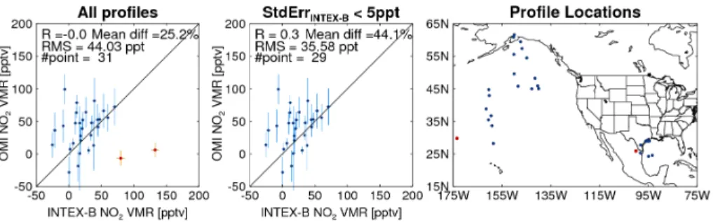
Figure 3 summarizes all comparisons between OMI and INTEX-B NO2 VMRs. We
analyzed all successful collocations of INTEX-B profiles and OMI cloud slicing NO2
VMRs and produced a scatter diagram in the left panel of Fig. 3. The vertical error bars are the 95 % confidence intervals of OMI NO2 VMRs, and the horizontal error bars
20
are the standard error of the mean of INTEX-B NO2 VMRs. The INTEX-B standard
error of the mean is small (.3 pptv) as compared with the magnitude of the NO2VMR, except for two cases that deviate significantly from the 1 : 1 line (∼6 pptv) marked in red color in the left panel of Fig. 3. The locations of the INTEX-B profiles are pre-sented in the right panel of the Fig. 3, with high standard error cases marked in red.
25
ACPD
14, 1559–1615, 2014Free tropospheric NO2from OMI cloud
slicing
S. Choi et al.
Title Page
Abstract Introduction
Conclusions References
Tables Figures
◭ ◮
◭ ◮
Back Close
Full Screen / Esc
Printer-friendly Version
Interactive Discussion
Discussion
P
a
per
|
D
iscussion
P
a
per
|
Discussion
P
a
per
|
Discuss
ion
P
a
per
|
differences≃36 pptv). In either case, the mean OMI VMR (36–39 pptv) is larger than
that of the INTEX-B VMR (22–27 pptv). These differences are in the same direction and general range (25–44 %) of the suspected OMI NO2SCD high bias (25 %).
Over-all, this comparison, even with its intrinsic limitations, provides some confidence in the ability to estimate NO2mixing ratios with OMI cloud slicing.
5
For comparison between OMCLDRR and OMCLDO2 results, a scattergram using OMI VMRs derived with OMCLDO2 cloud data is presented in Appendix D. OMCLDO2 results show similar magnitudes and scatter as compared with OMCLDRR. When we exclude the high standard error cases, OMCLDO2 data result in slightly higher scatter and lower correlation vs. INTEX-B.
10
4.2 Global seasonal climatology of free tropospheric NO2VMR
We construct a seasonal climatology of OMI free tropospheric NO2 as explained in
Sect. 3 and Appendix A2. In analyzing the global climatology, we focus on spatial and temporal variations of the NO2VMR rather than its absolute magnitude. In this section, we examine aspects of the OMI free tropospheric NO2 climatology in the context of
15
anthropogenic and lightning contributions. We also show GMI free tropospheric NO2
VMRs for comparison.
Details regarding the construction of the climatology are provided in Appendix A2. NO2 VMRs are not obtained where clouds rarely form (e.g., Sahara) or where cloud
pressure variability is small (e.g., oceanic areas with persistent low clouds due to
sub-20
sidence, such as offthe western coasts of South America and southern Africa). As we sample GMI output over the OMI cloud pressure range, we do not obtain GMI NO2
VMRs where OMI NO2 VMRs and the corresponding cloud pressure range are not
reported.
Here, we note the possible sampling biases in the NO2climatology. Since we collect
25
OMI measurements in cloudy scenes, the climatology represents NO2VMRs in highly
ACPD
14, 1559–1615, 2014Free tropospheric NO2from OMI cloud
slicing
S. Choi et al.
Title Page
Abstract Introduction
Conclusions References
Tables Figures
◭ ◮
◭ ◮
Back Close
Full Screen / Esc
Printer-friendly Version
Interactive Discussion
Discussion
P
a
per
|
D
iscussion
P
a
per
|
Discussion
P
a
per
|
Discuss
ion
P
a
per
|
indicative of those found in presence of frontal storms, where uplift of boundary layer pollution can frequently occur.
We use the standard error as an estimate of uncertainty for the derived NO2
climatol-ogy; this assumes that the error of the derived NO2VMR has zero mean and that errors for individual measurements are random and uncorrelated with respect to each other.
5
While these assumptions are not likely to strictly hold (there are indications of a bias), they may lead to reasonable uncertainties with respect to the derived spatial and tem-poral patterns. We show the NO2VMR climatology where the standard error<10 pptv
(if VMR<20 pptv) or 50 % (if VMR>20 pptv). For more details regarding quality as-surance, see Appendix C. In addition to the standard errors, we present auxiliary data
10
to help interpret the climatology, including the number of measurements, confidence intervals, standard deviations, and the mean cloud scene pressures corresponding to the NO2climatology in Fig. C1 of Appendix C.
Figure 4 shows global data averaged over June–August (left column) and December–February (right column) for 2005–2007. The first row shows the
OMI-15
derived 3 month seasonal climatology of free tropospheric NO2 VMRs. The second
row displays the GMI NO2VMRs in cloudy (τ >10) conditions, averaged over the cor-responding OMI cloud scene pressure range. The effect of clouds on NOx chemistry
is complex; it depends on altitude with respect to clouds. For example, NO2photolysis
rates may be increased above or within bright clouds, but decreased below them. In
20
general, the GMI cloudy VMRs are higher than those in all-sky conditions over urban regions and lower over remote and oceanic regions (see Fig. C2 in Appendix C). The third row shows lightning contributions to the free tropospheric NO2as taken from the GMI model. Note that we use a log scale for NO2 VMRs to highlight seasonal and
spatial variations. In Appendix C, we show additional NO2fields for reference including
25
GMI all-sky NO2 VMR, OMI tropospheric column NO2, and GMI tropospheric column NO2.
Be-ACPD
14, 1559–1615, 2014Free tropospheric NO2from OMI cloud
slicing
S. Choi et al.
Title Page
Abstract Introduction
Conclusions References
Tables Figures
◭ ◮
◭ ◮
Back Close
Full Screen / Esc
Printer-friendly Version
Interactive Discussion
Discussion
P
a
per
|
D
iscussion
P
a
per
|
Discussion
P
a
per
|
Discuss
ion
P
a
per
|
low, we examine the potential contributions from different sources by analyzing rough vertical profiles (Sect. 4.3) as well as temporal/spatial variations of free tropospheric VMRs (Sects. 4.2.1 and 4.2.2). Further analysis related to the differences between OMI and GMI free tropospheric NO2is ongoing.
4.2.1 Anthropogenic contributions
5
In the Northern Hemisphere (NH) winter (December–February), the primary source of free tropospheric NO2 appears to be anthropogenic emissions; high free tropospheric
VMRs are seen over densely populated regions and the lightning contribution is ex-pected to be negligible during these months (top right panel of Fig. 4). Over most of the highly populated areas of North America, southeast (SE) Asia, and Europe, free
10
tropospheric NO2VMRs are higher in winter (December–February) as compared with summer (June–August). It is well known that boundary layer NO2VMRs are generally
higher in winter as compared with summer owing to a longer chemical lifetime in winter; the OMI-derived tropospheric columns (the first row of Fig. C3 in Appendix C), that are dominated by boundary layer pollution in heavily populated areas, also reflect higher
15
values in winter than in summer. In contrast to NO2VMRs from OMI, the NO2 VMRs
from GMI are higher in summer as compared with winter over southeast Asia (the sec-ond row of Fig. 4 for cloudy csec-onditions, and Fig. C2 for all-sky csec-onditions), while the tropospheric column NO2 from GMI is higher in winter in this region (the second row
of Fig. C3 in Appendix C). Examination of GMI NO2and NO vertical profiles confirms
20
that this is not a simple partitioning problem of NOx.
Overall, OMI NO2 VMRs have lower values in the SH during the austral winter as
compared with the NH. This is also shown in the GMI output. It should be noted that there are not many large population centers in the SH, particularly at high latitudes, nor as much NOx contribution from aircraft at high latitudes in the SH as compared
25
ACPD
14, 1559–1615, 2014Free tropospheric NO2from OMI cloud
slicing
S. Choi et al.
Title Page
Abstract Introduction
Conclusions References
Tables Figures
◭ ◮
◭ ◮
Back Close
Full Screen / Esc
Printer-friendly Version
Interactive Discussion
Discussion
P
a
per
|
D
iscussion
P
a
per
|
Discussion
P
a
per
|
Discuss
ion
P
a
per
|
Africa and Sao Paulo, Brazil) owing to a lack of optically thick clouds and/or cloud pressure variation.
Regarding transport of anthropogenic NO2, we focus on winter months when
light-ning NO2 contributions are likely to be small. The OMI cloud slicing NO2 climatology shows a spatial patterns consistent with pollution outflow from North America and Asia.
5
For example, the persistent Asian northeasterly outflow of NO2via the Bering Sea
re-sembles that of CO (e.g., Liang et al., 2004), a tracer of incomplete combustion emis-sions. The spatial extents of continental outflows are different for the free tropospheric VMRs and tropospheric columns. This might be explained by extended transport at higher altitudes where the NO2lifetime is longer.
10
4.2.2 Lightning contributions
A band of enhanced NO2 appears extensively during the summer in the both
hemi-spheres (∼0–30◦ and possibly higher latitudes in the NH). The low cloud scene pres-sures (shown in the fifth row of Fig. C1 in Appendix C) in these regions are indica-tive of frequent convection. In particular, extensive enhancements in summertime NO2
15
VMRs over NH tropical and subtropical oceans, are similar to modeled lightning NOx
enhancements in previous studies (e.g., Choi et al., 2008; Allen et al., 2012; Martini et al., 2011; Walker et al., 2010). This suggests that lightning is a major source of free tropospheric NO2 in tropical and subtropical regions in summer. Because the SH is
far less polluted than the NH, potential NO2 enhancements due to lightning are more
20
apparent there. Finally, we note that these extensive NO2 enhancements indicated by cloud slicing during summer over oceans are not as apparent in the OMI tropospheric columns.
While the locations of these apparent lightning-enhancements of NO2 are similar in summer in both GMI and OMI data sets, there are a few key differences to note. For
25
example, the seasonality of the NO2enhancements over oceans shown by OMI is not
ACPD
14, 1559–1615, 2014Free tropospheric NO2from OMI cloud
slicing
S. Choi et al.
Title Page
Abstract Introduction
Conclusions References
Tables Figures
◭ ◮
◭ ◮
Back Close
Full Screen / Esc
Printer-friendly Version
Interactive Discussion
Discussion
P
a
per
|
D
iscussion
P
a
per
|
Discussion
P
a
per
|
Discuss
ion
P
a
per
|
For comparison, we also show maps of free-tropospheric NO2climatology obtained with OMCLDO2 cloud data in Fig. D2 of Appendix D. The OMCLDO2 climatology shows very similar spatial and temporal patterns as compared with that derived us-ing OMCLDRR data presented here with slightly lower VMRs in general. However, the OMCLDO2 climatology does not show a strong signature of lightning-enhanced NO2
5
over the tropical North Pacific in June–August as is shown in the OMCLDRR climatol-ogy. This is discussed in more detail in Appendix D.
4.3 Profile analysis
We examine the pressure dependence of the derived VMRs over large regions (to re-duce random errors) in order to provide a rough vertical distribution of free tropospheric
10
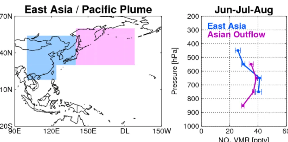
NO2. We highlight two types of areas: (1) East Asia and its outflow region to focus on anthropogenic contributions, and (2) tropical portions of the NH and SH to examine potential lightning contributions.
Figure 5 shows NO2profiles obtained over East Asia and its outflow region in sum-mer 2005–2007; in this region and season, a large number of cloudy pixels are
avail-15
able and cloud pressures exhibit enough variability to construct profiles due to the large sampling area and monsoon. This is not the case for many other urban regions and seasons. The sampling areas are shown in blue (East Asia) and purple (outflow) on the maps, and the corresponding profiles are presented in the same colors. The standard errors are also shown and are relatively small owing to the large number of samples.
20
We note that NO2profile information is not obtained in the lowermost troposphere over East Asia; we attempt to avoid boundary layer contamination in order to preserve the assumption of uniform NO2VMRs over the observed cloud pressure range. We obtain
a profile down to 850 hPa in the outflow region because there is little boundary layer pollution in that area.The profile of East Asia clearly indicates the presence of uplifted
25
anthropogenic NO2 in the middle troposphere of 600–800 hPa. In the outflow region,
ACPD
14, 1559–1615, 2014Free tropospheric NO2from OMI cloud
slicing
S. Choi et al.
Title Page
Abstract Introduction
Conclusions References
Tables Figures
◭ ◮
◭ ◮
Back Close
Full Screen / Esc
Printer-friendly Version
Interactive Discussion
Discussion
P
a
per
|
D
iscussion
P
a
per
|
Discussion
P
a
per
|
Discuss
ion
P
a
per
|
suggests that there is not a significant surface source NO2, and that uplifted anthro-pogenic NO2is transported at around∼700 hPa or above in this region.
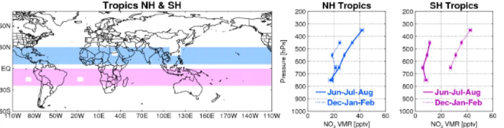
Figure 6 shows variations in the derived NO2profiles in tropical regions of the NH and
SH. Here, we examine two latitudinal bands with enhanced summertime NO2based on the spatial distributions shown in Fig. 4. Again, owing to the large number of samples,
5
the standard errors are relatively small (∼5 pptv). In summer, the NO2VMRs increase
with altitude in both hemispheres. The profile shapes suggest that NO2sources, pre-sumably lightning, are located primarily in the upper troposphere in these regions. This is consistent with aircraft measurements (e.g., Huntrieser et al., 2009) and modeling studies (e.g., Allen et al., 2010, 2012; Martini et al., 2011) of lightning-generated NOx.
10
In contrast, NO2 VMR profiles are more uniform in winter, possibly owing to less fre-quent lightning activity associated with convection in the shifting Inter-Tropical Conver-gence Zone (ITCZ). We note that the winter baseline NO2 VMR is higher in NH by
approximately a factor of two possibly due to more pollution sources in NH. In contrast, the summertime profiles of NO2are very similar in the NH and SH.
15
Overall, our analysis indicates a capability of the cloud slicing technique to retrieve NO2 profile information when provided with a relatively large sample size. Our profile results are consistent with an anthropogenic source for the enhanced NO2 in middle
to high latitudes offthe coasts of highly populated areas. They also indicate a lightning source in the summer over tropical areas, primarily located in the upper troposphere.
20
4.4 Stratospheric column NO2
We generated estimates of stratospheric NO2 columns as described in Sect. 3. As
done for the free tropospheric NO2 VMRs, the derived stratospheric columns of NO2
are averaged for 3 month intervals using data collected from 2005–2007. Zonal means are shown as a function of latitude in Fig. 7. We also show the estimates of
strato-25
spheric NO2 columns from OMNO2B (derived using a completely different method as
ACPD
14, 1559–1615, 2014Free tropospheric NO2from OMI cloud
slicing
S. Choi et al.
Title Page
Abstract Introduction
Conclusions References
Tables Figures
◭ ◮
◭ ◮
Back Close
Full Screen / Esc
Printer-friendly Version
Interactive Discussion
Discussion
P
a
per
|
D
iscussion
P
a
per
|
Discussion
P
a
per
|
Discuss
ion
P
a
per
|
from GMI in all seasons. Note that both OMI estimates are ∼30 % higher than GMI;
this is consistent with the expected high bias described in Sect 2.1.2. The overall excel-lent agreement between the cloud-slicing stratospheric column and other independent estimates provides a closure check on the derived free tropospheric NO2 VMRs; if the cloud-slicing procedure was not performing well in the free troposphere, we would
5
not obtain reasonable stratospheric column estimates. Therefore, this exercise pro-vides validation of both stratospheric and free tropospheric results. Estimates of strato-spheric columns from OMCLDO2 product display similar zonal structure as compared with those from OMCLDRR (not shown).
5 Conclusions
10
We have estimated free tropospheric NO2VMRs and stratospheric NO2columns using
a cloud slicing approach applied to OMI data from 2005 to 2007. Optically thick clouds provide excellent sensitivity of satellite radiances to NO2 above the cloud scene pres-sure; they also effectively shield satellite observations from NO2below clouds. In order
to retrieve NO2VMRs, our approach requires a large number of cloudy measurements
15
with substantial cloud pressure variability.
We conducted a detailed comparison between OMI cloud slicing free tropospheric NO2 VMRs and INTEX-B aircraft in situ measurements. Our analysis shows that the
cloud slicing technique provides similar magnitudes as compared with in situ measure-ments when known satellite biases are taken into consideration. However, individual
20
comparisons of INTEX-B and cloud slicing NO2 VMRs do not always exhibit good
agreement. Small-scale temporal and spatial variability, poor collocation, and fairly large OMI measurement uncertainties contribute to these discrepancies.
We generated global seasonal maps of free tropospheric NO2 VMRs as well as
free tropospheric NO2 vertical profiles over selected regions. With appropriate data
25
ACPD
14, 1559–1615, 2014Free tropospheric NO2from OMI cloud
slicing
S. Choi et al.
Title Page
Abstract Introduction
Conclusions References
Tables Figures
◭ ◮
◭ ◮
Back Close
Full Screen / Esc
Printer-friendly Version
Interactive Discussion
Discussion
P
a
per
|
D
iscussion
P
a
per
|
Discussion
P
a
per
|
Discuss
ion
P
a
per
|
slicing VMRs are fairly large; however, averaging over nine months (3 months×3 yr)
re-duces random errors and provides a reasonable estimate of the mean values. The free-tropospheric NO2VMR climatology shows distinct spatial and seasonal patterns; these
patterns differ from those of OMI-estimated tropospheric NO2 columns. The combina-tion of mapped and profile analyses indicates that spatial patterns of the OMI-derived
5
free tropospheric NO2are consistent with (1) uplifted anthropogenic NO2over densely
populated regions; (2) continental outflow of anthropogenic NO2; and (3) lightning-generated NOx, particularly in summer months at low to middle latitudes with a source
located primarily in the upper troposphere. Anthropogenic sources appear to dominate in the winter hemisphere, especially in the Northern Hemisphere at high latitudes near
10
heavily populated regions, while lightning contributions dominate over ocean at low to middle latitudes in summer in both hemispheres.
GMI model simulations suggest that NO2VMRs vary with cloud conditions by altering
the photochemistry. Spatial patterns of continental outflow show general agreement between the OMI cloud slicing climatology and GMI simulations for cloudy conditions.
15
However, some differences, particularly with respect to lightning-generated NOx, were
noted.
We also provided estimates of NO2 stratospheric columns from the cloud slicing
technique. These estimates agree well with those from the OMNO2B algorithm that are based on a completely independent technique (NO2 columns over clean regions).
20
The two OMI stratospheric NO2estimates display similar seasonal and latitudinal zonal
mean variations. These variations are also consistent with those produced in GMI sim-ulations. The excellent agreement between these stratospheric column NO2estimates provides a closure validation of the free tropospheric OMI cloud slicing results.
Our overall analysis shows that the cloud slicing technique can provide valuable
25
ACPD
14, 1559–1615, 2014Free tropospheric NO2from OMI cloud
slicing
S. Choi et al.
Title Page
Abstract Introduction
Conclusions References
Tables Figures
◭ ◮
◭ ◮
Back Close
Full Screen / Esc
Printer-friendly Version
Interactive Discussion
Discussion
P
a
per
|
D
iscussion
P
a
per
|
Discussion
P
a
per
|
Discuss
ion
P
a
per
|
North America (Chance et al., 2013) and the Korean Geostationary Environment Mon-itoring Spectrometer (GEMS) over the Asia–Pacific region (Kim, 2012). These missions should provide excellent cloud slicing results; they will provide improved sampling (with higher spatial and temporal resolutions) as compared with OMI.
Appendix A
5
Additional details in applying the cloud slicing technique
A1 Data filtering criteria
We apply the following checks to ensure that only high quality data are used in our analysis. With these checks, approximately 10–15 % of OMI pixels are retained, de-pending on season and geolocation: (1) we use only pixels withfr>0.9 to remove OMI
10
pixels with an insufficient cloud shielding of the boundary layer; (2) we remove data with aerosol indices>1.0, because absorbing aerosols are known to produce biases in the retrieved cloud properties (Vasilkov et al., 2008); (3) we exclude data with solar zenith angles (SZA)>80◦; the use of the geometrical AMFs may not be appropriate at higher SZAs owing to higher amounts of Rayleigh scattering; (4) we exclude data
15
affected by snow and ice because UV/VIS cloud measurements cannot differentiate between snow/ice and clouds; In the presence of snow/ice, we cannot be assured of boundary layer cloud shielding. We use a flag for snow- and ice-covered pixels based on the Near-real-time SSM/I EASE-grid daily global Ice and snow concentration and Snow Extent (NISE) data set (Nolin et al., 1998) provided in OMCLDRR product.
20
We also apply checks to ensure sufficient cloud variability; we only use collections with at least 30 OMI pixels, a cloud pressure standard deviation>35 hPa, and a cloud pressure range >200 hPa. Finally, we employ outlier checks to remove data that fall outside the range expected from our assumptions including a uniform mixing ratio over the appropriate pressure range and homogeneous stratospheric column over the
ACPD
14, 1559–1615, 2014Free tropospheric NO2from OMI cloud
slicing
S. Choi et al.
Title Page
Abstract Introduction
Conclusions References
Tables Figures
◭ ◮
◭ ◮
Back Close
Full Screen / Esc
Printer-friendly Version
Interactive Discussion
Discussion
P
a
per
|
D
iscussion
P
a
per
|
Discussion
P
a
per
|
Discuss
ion
P
a
per
|
responding area; we empirically selected a threshold of 2σ from the linear fit for this check.
A2 Application of cloud slicing to seasonal climatology
In order to create a global seasonal climatology of free-tropospheric NO2 VMRs, we
average individual retrievals in three month segments (one for each season) using
5
data collected over 3 yr (2005–2007). We grid the data at a spatial resolution of 6◦ lati-tude×8◦ longitude.
In Fig. A1, we show two examples of how the NO2 VMRs are calculated for a single
grid box. For these examples, we use only one month in summer (June) and winter (January). The grid box encompasses New York City, NY, USA. In order to remove
pix-10
els affected by substantial vertical gradients in the NO2VMR, we use only cloudy data
withPscene<a lower boundary (Plower, gray lines) where the mean NO2vertical profile
is relatively well mixed according GMI; specifically,Plower is pressure above which the
absolute magnitude of vertical gradient of monthly-mean NO2VMR<0.33 pptv hPa
−1
. Note thatPlower varies with season (as shown in Fig. A1) and geolocation (not shown).
15
For reference, we also show GMI daily and monthly mean profiles.
Using an OMI pixel collection from a single orbit, we calculate the free tropospheric NO2VMR (small black dots), the confidence interval (horizontal bars), and the pressure range (vertical bars). Then, we average the derived single-orbit NO2VMRs (weighted
inversely by the square of the confidence intervals) to obtain a single representative
20
NO2VMR for the given time period (large black dots).
In Fig. A1, we have shown data from one month for simplicity. To construct a seasonal climatology, we use the same spatial grid but a larger temporal window (3 months×3 yr) to reduce the sampling biases and random noise. For quality control of the clima-tology, we show data only where the NO2 VMR standard error of the mean <50 %
25
for NO2 VMR>20 pptv or NO2 VMR standard error of the mean <10 pptv for NO2
VMR≤20 pptv. With these criteria, there are some areas with no OMI-derived NO2
ACPD
14, 1559–1615, 2014Free tropospheric NO2from OMI cloud
slicing
S. Choi et al.
Title Page
Abstract Introduction
Conclusions References
Tables Figures
◭ ◮
◭ ◮
Back Close
Full Screen / Esc
Printer-friendly Version
Interactive Discussion
Discussion
P
a
per
|
D
iscussion
P
a
per
|
Discussion
P
a
per
|
Discuss
ion
P
a
per
|
with ice/snow. A similar approach is used to obtain gridded values of the stratospheric NO2column.
Appendix B
Additional case studies of OMI and INTEX-B comparisons
We show additional comparisons in which OMI and INTEX-B NO2 VMR display poor
5
agreement. These discrepancies are presumably caused by small-scale spatial and temporal variations in NO2 VMRs, different cloud conditions that might alter the NOx
photochemistry, and/or poor collocations.
Figure B1 shows a case with discrepancies likely due to the differences in the loca-tions, times, and the spatial scales of the measurements. The DC-8 profile was taken
10
over a small area near Houston in the morning (∼8.35 a.m. LT), while the OMI pixel collection covers a large area over Louisiana in the afternoon (∼1.35 p.m. LT) on the
same day; thus the OMI and DC-8 measurements were taken in adjacent locations with a∼5 h time gap. The DC-8 NO2 profile (second column) appears to be affected
by local pollution in the 600–800 hPa range. In contrast, OMI retrieves a low NO2VMR
15
over a wide area that includes less populated regions. OMI and INTEX-B VMRs show a significant difference of∼50 pptv in this case.
Figure B2 shows an example of small scale spatial variations in NO2profiles as seen by the aircraft measurements. The second column of Fig. B2 shows two DC-8 NO2
profiles that were taken on the same day at nearby locations. The first column shows
20
the two corresponding OMI pixel collections closest to the DC-8 profiles. In order to differentiate the two cases, the first row uses dark blue for tne DC-8 profile and light blue for OMI pixels, and the second row uses red for the DC-8 profile and pink for OMI pixels. Since the two DC-8 profiles encompass many of the same OMI pixels, the shared pixels are marked with purple on the map (top right). Although the two DC-8
25