c
European Geophysical Society 2001
and Earth
System Sciences
The pecularities of shear crack pre-rupture evolution and
distribution of seismicity before strong earthquakes
D. Kiyashchenko and V. Troyan
Physics Department, St. Petersburg State University, 1 Ulianovskaya Street, St. Petersburg, 198 504, Russia Received: 15 May 2001 – Revised: 30 September 2001 – Accepted: 17 October 2001
Abstract. Several methods are presently suggested for in-vestigating pre-earthquake evolution of the regions of high tectonic activity based on analysis of the seismicity spatial distribution. Some precursor signatures are detected before strong earthquakes: decrease in fractal dimension of the con-tinuum of earthquake epicenters, cluster formation, concen-tration of seismic events near one of the nodal planes of the future earthquake, and others. In the present paper, it is shown that such peculiarities are typical of the evolution of the shear crack network under external stresses in elas-tic bodies with inhomogeneous distribution of strength. The results of computer modeling of crack network evolution are presented. It is shown that variations of the fractal dimension of the earthquake epicenters’ continuum and other precursor signatures contain information about the evolution of the de-struction process towards the main rupture.
1 Introduction
The observations of spatial and temporal seismicity patterns play an important role in earthquake long-term forecasting. Several precursor phenomena were observed and studied be-fore strong earthquakes: the decrease in b-values (Suyehiro et al.,1964; Smith, 1981), the appearance of zones of seismic quiescence, where the seismicity level was weaker than in the surrounding area (Wyss and Haberman, 1988; Wyss and Haberman, 1997), and the power-law increase in the cumu-lative energy of earthquakes (Bowman et al., 1998; Brehm and Braile, 1998; Jaume and Sykes, 1999; Main, 1999; Robinson, 2000). In addition, the seismicity clustering was observed before strong earthquakes (Zavialov and Nikitin, 1999; Giombattista and Tyupkin, 1999). In addition, accord-ing to descriptions of laboratory experiments and seismic-ity observations, acoustic emission and seismicseismic-ity hypocen-ters tend to concentrate close to the nodal plane of a future Correspondence to:D. Kiyashchenko
main rupture. In this connection, the laboratory experiments of Mogi and Scholz ought to be mentioned (Mogi, 1968; Scholz, 1968). Moreover, the same pattern was observed in the seismicity behaviour of the Kamchatka region before some strong earthquakes (Zavialov and Nikitin, 1999). The formation of spatio-temporal clusters of acoustic emission, and hypocenter concentration close to the nodal plane of the main rupture were observed in the laboratory experiment by Sobolev and Ponomarev (1999).
These precursor phenomena have one important property: the evolution of spatial inhomogenity of the seismicity dis-tribution in a wide range of scales. A suitable method of description of the inhomogenity of the seismicity spatial dis-tribution is based on a fractal approach. The results of corre-sponding investigations show that seismicity has statistically self-similar properties in a wide range of scales. Therefore, it can be treated as fractal or multifractal. Several papers are related to this item (Sadovsky et al., 1984; Okubo and Aki, 1987; Geilikman et. al, 1990; Hirata and Imoto, 1991; Hi-rakashi et al., 1992; Turcotte, 1993; Wang and Lee, 1996; Lapenna et al., 2000). However, only few papers are re-ported, where the dynamics of fractal properties of seismicity were studied before strong earthquakes.
The gradual decreasing of the correlation exponent of the spatial distribution of acoustic shocks was observed by Hirata et al. (1987) during the destruction of granite sam-ple. The correlation exponent is a kind of fractal dimen-sion, which can be calculated for the group of points ac-cording to the following algorithm. LetN (R)be the num-ber of pairs of points, which are characterized by mutual distance, which does not exceedsR. Then, if the relation log(N (R))=b−alog(R)is true (the distribution of points has a fractal structure),ais called the correlation exponent. The calculation of the correlation exponent is more suitable for the analysis of small sets of data than the calculation of fractal dimension by the box-counting method.
ma-Fig. 1. The edge of the crack. R, θ are polar coordinates of the point in the local coordinate system linked to the edge of the crack (x1, x3).
terials of the world-wide seismicity data center were pro-cessed. The fractal dimension was calculated for the two-year period before and after 23 strong earthquakes. In 16 out of 23 cases, the pre-earthquake period was characterized by a lower fractal dimension.
Hence, the evolution of the inhomogenety of spatial dis-tribution of seismicity in different scales, manifesting itself as a decrease in fractal dimension, can be interpreted as a signature of the earthquake preparation process.
It is necessary to mention recent studies, dealing with the precursor phenomena, which are not connected directly with the evolution of the inhomogenity of spatial distribution of the seismicity. The observation of these precursor phenom-ena gave the evidence of the intensifying of long-range spa-tial correlations in the seismicity prior to mainshock.
Zoller and Hainzl (2001) observed the growth of the corre-lation length of seismicity prior to the main strong California earthquakes. The correlation length was calculated for the events, occurring within a sliding time window, by using sin-gle link cluster (SLC) analysis, described in Sect. 3 of the present paper.
Shebalin et al. (2000) studied the manifestation of long-range correlations in the seismicity according to the al-gorithm, described below. The distance was assigned as
R(i, j, τ )between the events with numbersiandj, which occurred within the time intervalτ. The considered events were not supposed to be weak (with magnitudeM > M0).
The distribution function of R(i, j, τ ) was studied for a six-month period before (D-intervals) and after (N-intervals) strong earthquakes. The authors found that the values of the distribution function corresponding to upper values of
R(i, j, τ )were larger for intervalsN. It means that the com-parative amount of events, situated within the mutual dis-tance, larger thanR, was higher for intervalsD(for the case of comparatively high values ofR(i, j, τ )). Therefore, the long-range correlations in seismicity are more intensive for the pre-earthquake periods.
The present paper contains the results of a numerical sim-ulation of the destruction of a mechanically inhomogeneous elastic body with a number of cracks. The effects of synthetic seismicity clustering, the behaviour of fractal dimension, the appearance of long-range correlations and manifestation of other precursor phenomena during the destruction process are discussed. It is shown that such precursor phenomena,
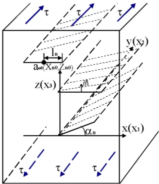
Fig. 2.The group of cracks of mode 3 in the volume of elastic body. τis the external stresses;x(x1), y(x2), z(x3)represent the
coordi-nate system.an0(xn0, yn0)represents the position of the crack with
the numbernon the complex plane;αn is the angle between the
crack plane and the axisx1;lnis the half of the crack length.
observed in the experiments, must be typical for the destruc-tion of elastic bodies containing a number of cracks.
The second part contains the description of the model of an elastic body with cracks under external stresses and the results of studying crack interaction. The role of crack inter-action in spatial organizations of seismicity is discussed.
The third part deals with the simulation of the destruction process and the study of the dynamics of the properties of synthetic seismicity.
2 The model of shear cracks in the elastic body under external stresses
It is well known that the origin of an earthquake is the de-struction of rocks under increasing tectonic stresses. The stresses lead to a growth of initial small cracks, causing the release of elastic wave energy during earthquakes. Hence, it is important to study crack network evolution under exter-nal stresses in order to understand the earthquake preparation process.
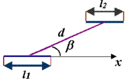
Fig. 3.dis the distance between the centers of the two cracks;βis the angle betweenx-axis and the line, connecting the centers of the cracks.
Such a model is mathematically simple. It allows us to make the numerical calculations for cases with large numbers of cracks in the network. In spite of its simplicity, this model reproduces the main features of the evolution of a network of cracks of more general types.
When the external stresses in elastic media reach some critical value, some cracks begin their rapid propagation. Hence, it is necessary to define the criteria for the beginning of crack propagation.
This criteria is based on the consideration of the stresses near the crack edge. In the general case, the stress tensor components near the edge (Fig. 1) of the crack can be written as follows (see Lawn and Wilshaw, 1977; Liebowits, 1968):
σij(R, θ )= 1 √
2R
3
X
m=0
Kmfijm(θ ) , (1)
whereKmrepresents the stress intensity factors, depending on the applied loading, and on the crack geometry;fij(θ )is the function of latitude angleθ.
Let us consider the crack of general type and select the local Cartesian coordinate system near its edge, as it is shown in Fig. 1. Then the stress tensor components will obey to the relations:
[σ33, σ13, σ23](R, θ )|θ=0= [
K1, K2, K3]
√
2R , (2)
which can be treated as the definition of the stress intensity factors.
The presence of an infinite stress value in the crack tips (1) is the result of the model simplifying. It was assumed that the crack tip in an unstressed state is absolutely sharp, and the crack walls are free of traction. It can be shown that the stresses near the crack edge are finite, if the traction forces (of atomic origin) between the crack walls near its tips are taken into consideration (Dugdale-Barenblatt “thin zone” model). In the case of brittle solids, the estimation of the size of zone, where traction forces are applied, gives the value of the or-der ofnm. Therefore, the presence of such a zone can be neglected for macroscopic cracks. Hence, Eq. (1) gives an exact description of the stress distribution near the edge of macroscopic crack.
The criteria for the beginning of crack growth can be de-rived using the law of energy conservation for elastic media
near the crack tip (see Lawn and Wilshaw, 1977). Let us imagine that the increment of the square of crack surface has the valuedS. Then, in the case of plane stress, the ratio of the strain energy releasedW to the valuedScan be written as follows:
G= dW dS =
(1−ν)
2µ
K12+K22+ 1
2µK
2
3, (3)
whereνis Poisson ratio,µis the shear modulus.
The criteria for the beginning of crack propagation is given by the equation:
G=2γ , (4)
where 2γ is the amount of energy that is necessary for the creation of the unit of crack surface (Griffith criteria).
Here we consider the problem of equilibrium of elastic volume with shear antiplane cracks (Fig. 2). The cracks, stresses and displacements are parallel to they-axis, and the displacements do not depend on they-coordinate:
u(x, y, z)≡u2(x, z)ey.
Then, using the well-known relation:
σij =λdivuδij +µ[
∂ui
∂xj +
∂uj
∂xi]
,
we can infer that the stress tensorσijhas only four non-zero components:
σ23=σ32=µ
∂u2
∂x3;
σ21=σ12=µ
∂u2
∂x1
. (5)
Here, the numbers 1, 2, 3 correspond to the coordinates
x, y, z;λ, µare Lame parameters;δij =1(0)ifi=j (i6=
j ).
According to the Eqs. (2) and (4), only the third stress in-tensity factorK3in Eq. (2) has a non-zero value. The criteria
for the beginning of antiplane crack propagation has a simple form:
K3=K3c, (6)
whereK3c is the critical stress intensity factor. Hence, it is sufficient to find the stress intensity factors near the crack tips to determine the beginning of crack propagation.
Taking into consideration the equations of equilibrium of elastic volume:
∂σi1
∂x1 +
∂σi2
∂x2 +
∂σi3
∂x3 =
0, (i=1,3),
we can conclude that the displacementsu(x1, x3)obey the
Laplace equation:
∂2u ∂x12 +
∂2u
∂x32 = 0. (7)
The external stressτ is supposed to be applied remotely from the crack plane:
σ23|z=±∞=µ
∂u ∂z
z=±∞
The stressτf, caused by friction forces, can be applied to the surfaceSnof the crack with numbern. The correspond-ing boundary condition can be written as:
3
X
i=1
σ2ini
S n
=µ ∂u ∂m Sn
=τf, (9)
wheremis the normal vector to the crack surface. The displacements can be decomposed as:
u=u0+u1,
where u0 is the solution of equivalent problem (6), (7) of
equilibrium of elastic media without crack:
u0=
τ z µ .
Then the displacementu1can be found from the solution
of the following problem:
1u1=0 (10)
∂u1 ∂m Sn=
− τ m3−τf
µ (11) ∂u1 ∂z z=±∞
=0. (12)
Consideration of the role of friction forces in this model can be reduced by their subtraction from external stresses, if the cracks are assumed to be subparallel (m3 =0). Below,
we assume that the friction stressτf vanishes.
The problems (9–11) can be solved using methods of the theory of functions of a complex argument, elaborated by Kolosov and Mushelishvilli (the solution can be found in Ap-pendix A).
The stress intensity factorsK3n±near the tips of the cracks
with numbersn = 1,..., N (Fig. 2) can be found from the solution of the system of integral equations:
Gn(yn)= − 1
π√ln ln
Z
−ln
p
l2
n−x2τn (x)
x−yn
dx
+ 1
π√ln
X
k6=n lk
Z
−lk √
lkGk(x)
q
lk2−x2
Mnk(xn, x) dx
Mnk(y, x)=Re
1+ q
cnk2 −l2
n
yn−cnk
;
cnk =
exp (iαk) x+ak0−an0
exp (iαn)
(13)
K3n±= |Gn(±ln)|.
Here an0 is the position of the crack center on a complex
plane,αn is the angle between the crack plane and the axis
x1,ln is the half of the crack length,nis the crack number, −ln< yn< ln, the sign+(−)corresponds to the right (left) tip of the crack.
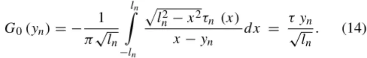
Assuming that the external stressτdoes not depend on the
x-coordinate, the first integral in (12) can be written as:
G0(yn)= − 1
π√ln ln
Z
−ln
p
l2
n−x2τn(x)
x−yn
dx = τ y√n ln
. (14)
The system of integral equations (12) can be solved by the iteration method. The initial approximation is given by the expression (13) for G0(yn). The study of influence of one crack on another is important for the understanding of the crack network behaviour. Let us consider two cracks(n =
1,2)with the lengthsln, the positionsxn, yn, and the angles
αn =0 (Fig. 2). Then, the ratio
mn±=
K3n±
K3one
can be the measure of interaction of the crack of numbern
with another crack, whereK3one=τ√lnis the stress - inten-sity factor, calculated for a single crack of the numbernin elastic media under the same external stresses. The value of
mn±shows the influence of the presence of another crack on
the stress intensity factors near the tip of the crack of number
n.
The dependence ofmn± on the positions of both cracks
was studied. The relative positions of both cracks are char-acterized by the distancedbetween the centers of two cracks and the angleβ, between thex-axis and the line, which con-nects the centers of the cracks (Fig. 3).
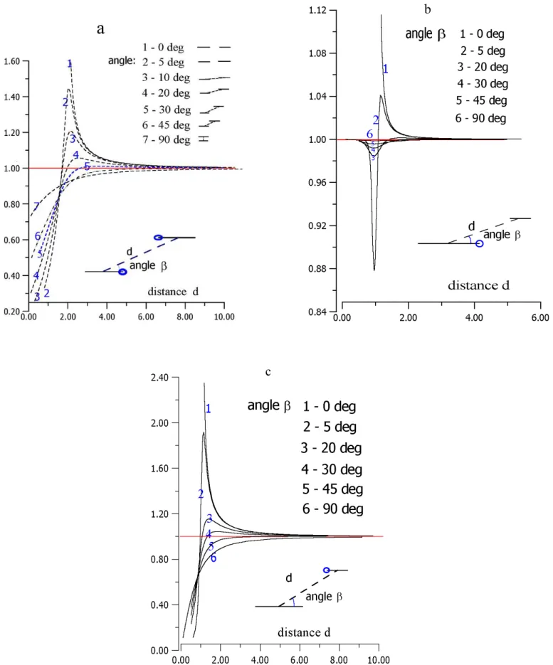
Figure 4a shows the results of calculation of the ratiom1+
for two equal cracks (l1 = l2 = 2). Figure 4b shows the
results of the calculation of the ratiom1+ for the right tip
of the first one of the non-equal cracks (l1 = 2; l2 = 0.2).
Figure 4c shows the behaviour of the ratiom2−for the left tip
of the second one of the non-equal cracks (l1=2; l2=0.2).
The results of the calculations allow us to infer some im-portant conclusions:
1. The effect of crack interaction can be neglected, if the distance between these cracks exceeds several crack lengths.
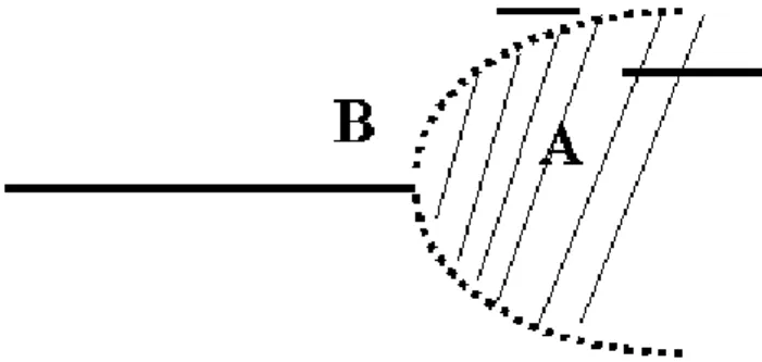
2. The stress intensity factor near the crack tip increases, if the crack is situated in zone A near another crack (Fig. 5). Therefore, the risk of destruction is compar-atively higher in zone A. The intensity coefficient has a maximal value when the crack is situated on the prolon-gation of another crack (angleβ= 0; Figs. 4a–c). 3. The stress - intensity factor near the crack tip decreases,
if the crack is situated in zone B near another crack (Fig. 5). The risk of destruction is comparatively lower there.
Fig. 4.The results of calculation of the ratiomn±for the following cases:(a)l1=l2=2,(b)l1=2;l2=0.2,(c)l1=0.2;l2=2;nare
Fig. 5.The domains of stress increase (A) and stress drop (B) near the crack.
Fig. 6. The results of calculation of maximum value of stress – intensity factorKmaxfor two different clusters
5. The influence of the smaller crack at the tip of the larger crack is significant, if the distance between crack tips is less than several lengths of the smaller crack (Fig. 4b). These facts allow us to judge the role of crack interaction in the spatial organization of seismicity:
1. The existence of stress-drop and stress-increase zones near the cracks explain the tendency of earthquake epi-centers to form spot-like fractal structures. Therefore, the fractal methods are suitable for monitoring the de-struction process evolution. The evolution of spot-like cluster structures of seismicity causes the decrease in fractal dimensions. The aforementioned behaviour of the fractal dimension of synthetic elastic shocks is shown and discussed in the third part of the present pa-per.
2. A specific form of zones of comparatively higher risk of destruction (Fig. 5) must cause an oblong structure of crack clusters. This explains the concentration of the seismicity and the acoustic shocks close to the plane of the main rupture before the mainshock (Mogi, 1968; Scholz, 1968; Zavialov and Nikitin, 1999; Sobolev and Ponomarev, 1999). On the other hand, the risk of crack propagation is higher in an oblong cluster of cracks. Figure 6 presents the results of the calculation of max-imum value of the stress intensity factorKmax for two different clusters. The long cluster shows a higher value ofKmax.
The model of shear cracks, studied in the present work, is simple. The cracks of a more complex type could be consid-ered: curvilinear, with various forms in a plane. The stresses could not be applied to the infinite boundary, but to the sur-face, situated on the finite distance from the crack plane.
Moreover, the displacements could be fixed on the boundary, instead of on the stresses.
However, it can be assumed that qualitative results, ob-tained for the crack network evolution model and presented in our paper, can reproduce the most principal features of the behaviour of more complex types of cracks.
The supporting arguments are the following:
1. The stress intensity factors near the tips of all cracks, situated in elastic media under uniform external stress, which are applied remotely from the crack plane, in general, obey the relation: K =mτ√a, whereais the size of crack,τis external stress value andmis a dimen-sionless magnification factor (see Lawn and Wilshaw, 1977).
2. The presence is evident of the domains of stress-drop and stress-increase near the cracks of different form. 3. When the crack is comparatively small, the influence
can be neglected of finite distance between the surface, where the boundary conditions are fixed, and the crack surface. The next results allow one to make such a con-clusion:
(a) The solution can be seen of the problem of equilib-rium of an elastic block with a crack, where the stresses are applied to the boundary (Panasuk et al., 1976). The influence of the boundaries becomes significant, if the crack length exceeds the quarter of the distance between the boundary and the crack plane.
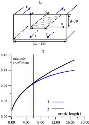
(b) Let us consider the crack of mode 3 with lengthlin the elastic block with fixed displacements on the bound-ary (Fig. 7a).
The displacementsu(x, z)must obey the equilibrium equa-tion:
1u = 0. (15)
The crack surface and the part of the boundary are sup-posed to be free of stresses:
σ23=µ
∂ u ∂ z
z=0;0<x<l
=0 (16)
σ13=µ
∂ u ∂ x
x=±w =0
. (17)
The displacements are fixed on another part of the bound-ary:
u|z=±d = ±u0= ±0.5. (18)
Fig. 7. (a)The crack of mode 3 in the elastic block with fixed displacements on the boundary;τ – the external stresses;(b)The results of calculating of the stress – intensity factor near the tip of crack versus the length of crackl(curve 1 – for the displacements, applied on the boundary; curve 2 – for the stresses, applied to the infinite boundary).
elastic volume under equivalent stresses (τ =u0/d), applied
remotely from the crack surface. The effect of the bound-aries is significant when the crack length exceeds the half of the distance between the boundary and the crack plane.
3 Simulation of the destruction process
We considered elastic volume withN subparallel cracks of mode 3, shown in Fig. 2. The increasing stresses were ap-plied to infinite boundary of the volume. The stress intensity factors near the crack tips were inferred from the solution of the system of integral equations (12) using first-order ap-proximation. The reliability of the first-order approximation is shown in Fig. 8. If the distance between the crack tips exceeds the crack length, the first-order approximation gives a quantitative estimate of crack interaction. In the opposite case, the first-order approximation gives a qualitative esti-mate of crack interaction.
It was assumed that the crack propagated if K > Kc, whereK is the stress intensity factor near the crack tip, and
Kc is the critical stress intensity factor. A real rock contain pores, microcracks, layers, contact zones. It can be seen from Fig. 4b that the influence of the presence of the small crack near the tip of a big crack can cause variations in the
stress-Fig. 8. The results of the calculation of the ratiom1+: curve 1 –
the exact solution; curve 2 – the solution, using only the first-order approximation.
intensity factor near its tip. If we do not take into account the cracks with extremely small size, their influence can be interpreted as a local variation ofKc. The presence of water in the media can also reduce the local rock strength. Hence, this allows us to consider that there are many levels ofKcin rocks: Kc1, Kc2, Kc3, . . . , Kcn. According to some estima-tions of the ratio (3) (see Rice, 1980), the variance ofKc in rocks can be assumed to be much larger than the variance of elastic modulus. This allows us to use the simplification of the homogeneous elastic media with highly inhomogeneous distribution of strength.
The elastic volume considered was divided into a number of parts. Each part was characterized by its ownKc. The different values ofKcwere randomly distributed in the me-dia. The number of blocksNb, characterized by critical stress intensity factorKc, depend on its value:
Nb(Kc)∝
const Kc
. (19)
Indeed, it is difficult to do any reasonable suppositions, in general, about the relative portions of domains in the elas-tic media with different values ofKc. The assumption (18) allowed us to obtain a sufficient number of synthetic elastic shocks during the simulation of the destruction process with-out consideration of the extremely high number of cracks.
The initial cracks were randomly distributed within the media. They had the lengthl = l0. According to the
with low values ofKc. This feature reproduces the evident tendency of cracks to appear in the domains of elastic media, characterized by low values of strength in the beginning of destruction process.
The stress was increased with constant velocityv0:
τ =v0t. (20)
The destruction process was stopped when both crack tips reached the border of the block.
The simulation was accomplished for the following model parameters:
– Block height: 10 cm;
– Block width: 10 cm;
– Number of cracks:N =600;
– Initial crack length:l0=0.02 cm;
– Critical stress intensity factor values: 0.1, 0.11, 0.12,..., 10. Mpa m1/2;
– Velocity of stress increase:v0=0.01 Mpa/s.
The manifestation of several precursor phenomena, observed in seismicity, was studied for a simulated destruction process. The results are summarized below.
1. Analysis of the dynamics of correlation dimension of spatial distribution of synthetic elastic shocks.
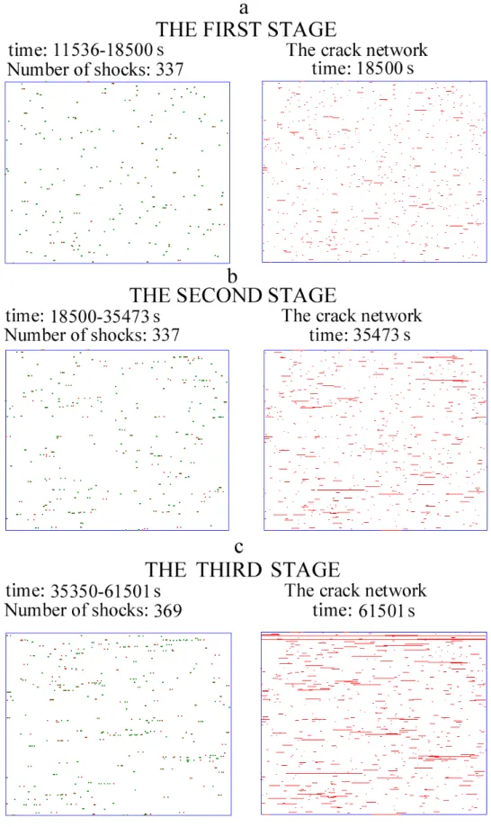
The destruction process was divided into three stages (stage 1: t = 11 536 −18 500 s, N = 337; stage 2: t = 18 500−35 473 s, N = 337; stage 3: t =
35 350−61 501 s,N=369), which had almost an equal number (N) of synthetic elastic shocks. This was nec-essary for stable estimation of the correlation exponents of the shock epicenters distribution.
The correlation exponents were calculated for these three stages using the linear part of the log-log depen-dence by the least square method. The nonlinear part of the log-log plot on the large scales appeared due to boundary effects. The same feature also occurred at small scales, due to the formation of clusters of syn-thetic shocks, produced by the development of one and the same crack.
The elastic shock distribution and the crack network at the end of each stage are shown in Figs. 9a–c.
The correlation exponents calculated for the three stages are, correspondingly,D1 = 1,68; D2 = 1.63; D3 =
1.58. The evolution of the cluster synthetic seismicity structure can be seen during the simulated destruction process. The minimal value of correlation exponent was observed before the main rupture moment.
Moreover, it can be seen that at the last stage, synthetic seismicity tends to concentrate close to the plane of fu-ture rupfu-ture. This fact is in agreement with the results of experiments mentioned in the Introduction to this paper.
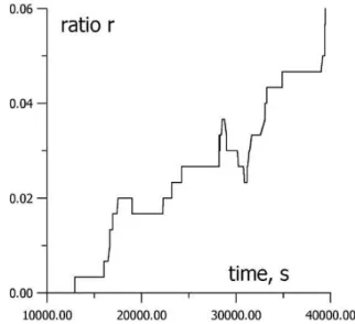
Fig. 10. The dynamics of the ratior = N (l > l0 = 0.5cm)/N0 during simulated destruction process. N (l > l0)is the number of
events, characterized by larger differential length of appeared crack thanl0.
Fig. 11. The dynamics of correlation length during simulated de-struction process.
2. Analysis of the dynamics of the relative number of synthetic elastic shocks with high magnitude.
The empirical relation M ∼ lg(E) ∼ lg(l) exists in seismology (see Sobolev and Ponomarev, 1999) be-tween the lengthlof earthquake rupture and its energy
E(magnitudeM). Therefore, the length of an appear-ing crack can be treated as a measure of the magnitude of the corresponding shock. The differential lengthlof the newly appeared crack, corresponding to a synthetic shock, was defined as the difference between the lengths of the crack after and before its propagation.
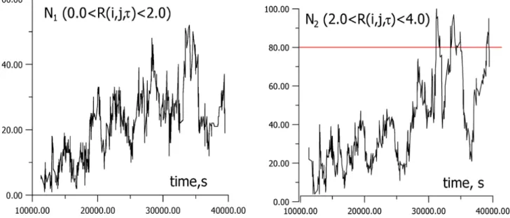
Fig. 12.The temporal variations of the numbersN1(a)andN2(b)of the pairs of events, situated within mutual distances 0< R(i, j, τ ) <2.
(a)and 2. < R(i, j, τ ) <4.(b), and occurred within time intervalτ.
high magnitude was defined forN0 events as the ratio
r = N (l > l0 = 0.5cm)/N0, whereN (l > l0)is the
number of events, for which the differential length of the appeared crack is larger thanl0.
The ratiorwas calculated for the events that occurred within the sequence of time intervalsTn≡(tn;tn+300).
Heretn is the time of occurrence of the event with the numbern, which changes in the limits (1, N −301), whereNis the number of all events obtained during the simulation of the destruction process. The dependence of the ratior versustn is shown in Fig. 10. A gradual increase ofrwas observed during the simulated destruc-tion process.
The increase in the relative number of shocks with high magnitude is in agreement with the decrease in b-values, observed in the seismicity prior to strong earth-quakes. The decrease in the slope of the crack size dis-tribution function was also reproduced by the model of Czehovski (1995), realizing the kinetic approach to the study of the crack network evolution. Due to a com-paratively small amount of events obtained during the simulation of the destruction process, the calculation of b-values was not performed in the present study.
3. Analysis of the dynamics of correlation length for synthetic elastic shocks.
The correlation length was calculated, using single-link cluster analysis (see Zoller and Hainzl, 2001). LetN0
be the whole amount of earthquakes. Each individual event is linked to its nearest neighbour event in space in order to form a set of small clusters. This process is repeated, recursively, untilN0events are connected by
N0−1 links. The distribution functionF (l)gives the
probability that the link length is smaller than or equal tol. The correlation lengthlcis defined by the condition
F (lc)=0.5.
The correlation lengthlc was calculated for the events that occurred within the sequence of time intervalsTn, each containing 300 events. The calculation of cor-relation length was performed for an equal number of shocks for stability of its estimation.
The dependence of correlation length lc versus tn is shown in Fig. 11. The correlation length increases rapidly at the beginning stage of the destruction process, and then oscillates near some constant value.
4. Analysis of the dynamics of spatiotemporal correla-tions in the seismicity.
In order to study the evolution of spatiotemporal cor-relations in the seismicity, we studied the dynamics of relative numbersN1(N2)of the pairs of events
sit-uated within mutual distance 0 < R(i, j, τ ) < 2.
(2. < R(i, j, τ ) < 4.), and occurred within temporal interval τ. Like Shebalin et al. (2000), we supposed that the events were not weak (the corresponding differ-ential length of the crack was supposed to be larger than 0.05 cm). The parameterτ =1 was supposed to be less than the ratio (tN−t1)
10N , wheretn,N has the same mean-ing, as in the previous point. The values ofN1(N2) were
calculated for the events, that occurred within the se-quence of time intervalsTn, each containing 300 events. The results of the calculation ofN1andN2for the
sim-ulated destruction process are shown in Figs. 12a and 12b, correspondingly. The behaviour ofN1is similar to
almost constant value. The dynamics ofN2 is another
one. At the beginning stage this value increases compar-atively slowly. But prior to the mainshock,N2increases
rapidly. This phenomena reveals the intensification of the long-range correlation in synthetic seismicity prior to the mainshock. Moreover, Figs. 12a and 12b demon-strate the temporal clustering of the synthetic seismicity during the evolution of the destruction process. This is in agreement with the observations of Sobolev and Ponomarev (1999).
The method, suggested by Shebalin et al. (2000), seems to be more efficient for studying long-range correla-tions, than a simple calculation of correlation length (Zoller and Hainzl, 2001), because it takes into consid-eration temporal correlations in the seismicity, in addi-tion to spatial distribuaddi-tion.
4 Discussion
The model of the earthquake preparation process, considered in the present paper, explains and reproduces the set of pre-cursor phenomena, including the changes in correlation di-mension of spatial distribution and the intensification of spa-tiotemporal long-range correlations in the seismicity.
At the beginning of the destruction process elastic shocks are linked to the domains of elastic media, characterized by low strength values. Such domains are supposed to be ran-domly distributed in elastic volume. Therefore, the correla-tion exponent had to be high at the beginning stage of the de-struction process (Fig. 9a). The cracks are growing and their interaction causes the formation of clusters of elastic shocks (Figs. 9b and 9c) in a wide range of scales. This causes the decrease in the correlation exponent.
The radius of interaction of growing cracks increases. Therefore, the cracks can induce the propagation of other cracks, situated further away from them. This is the reason for temporal clustering and appearance of long-range corre-lations in the seismicity during the crack network evolution.
Hence, the evolution of spatial inhomogenity of the seis-micity distribution and the appearance of long-range corre-lations have the same origin in the frame of the considered model and must be typical features of the destruction of elas-tic bodies containing a number of interacting cracks.
The decrease in the fractal dimensions of elastic shock dis-tribution and the appearance of long-range correlations can be interpreted as an indicator of the evolution of crack in-teraction during the destruction of the elastic volume. The results of the second part of this paper allow one to assume that the degree of intensity of the interactions of cracks in the network can be treated as the measure of the risk of the occurrence of rupture, since the crack interaction can cause strong variations in the stress-intensity factors near the crack tips.
Therefore, monitoring of the aforementioned peculiarities in spatial and temporal distributions of seismicity can give us
the information about the evolution of the destruction process in the Earth’s crust towards the main rupture.
In the present study, following Hirata et al. (1987), we used the correlation integral method for analysis of the spa-tial distribution of synthetic seismicity. Uritsky and Troyan (1998) studied the behaviour of fractal dimension, calculated by the box-counting method. The selection of the most ap-propriate method of analysis must depend on the kind of data set. However, the most common approach can be based on the multifractal theory. The analogy can be seen between the redistribution of stress in elastic volume during the crack for-mation processes and the redistribution of the measure in the multifractal process. Therefore, the application of multifrac-tal methods seems to be suitable for monitoring the destruc-tion processes.
Appendix A The solution of the problem of equilibrium of antiplane shear cracks in elastic volume under an-tiplane external stresses.
The problem of equilibrium of shear cracks of mode 3 is stated in Eqs. (9)–(11). A more general statement of this problem can be written as:
1u=0, (A1)
∂u ∂m
Sn
= τn(x)
µ , n=1, . . . , N (A2)
∂u ∂x3
x
3=±∞
=0. (A3)
Hereµis shear modulus;mis the normal vector to crack surface;τn(x)is shear stress, applied to the surfaceSnof the crack with numbern (Fig. 2); variable x (−ln < x < ln) represents the position of the point on the crack surface;ln is the half of the length of the crack. Taking into considera-tion Eqs. (A1) and using Koshi-Riman relaconsidera-tions, the problem (A1)–(A3) can be rewritten as:
u= Reϕ(z)
µ , (A4)
I mϕ′(z)S
n = −τn(x), n=1, ..., N (A5) I mϕ′(z)z
=±∞ =0, (A6)
where ϕ(z) is some function of a complex argument z = x1+ix3.
Hence, it is necessary to find the functionϕ(z). Let us imagine that we know the jump of the displacements on the crack surface:
[u]|Sn =u
+
n −u−n =
γn(x)
where +(−) corresponds to upper(lower) part of the crack surface. Then, taking into account that[I m(ϕ′(z))]
Sn =0, we can obtain the relation:
ϕ′(z+)−ϕ′(z−)=2γn′(x). (A8) The functionϕ(z), satisfying this relation for any crack, can be composed as:
ϕ′(z)= 1 π i
N
X
n=1
Z ln
−ln
γn′(x)
x−(z−an0)exp(−iαn)
dx, (A9)
wherean0 is the position of the crack center on a complex
plane;αnis the angle between the axisx1and the crack plane.
Let us select the coordinate system in such a way thatzn0
= 0 andαn=0 for the crack with numbern. Then:
ϕ′(z)= 1 π i
Z ln
−ln γn′(x)
x−zdx+G(z), (A10)
where G(z) is continuous function on the crack surface
(G+(z)=G−(z)). According to Plemel’s theorem, if
ψ (z)= 1
2π i
Z l
−l
g(x) x−zdx,
then
ψ (z±)= ±g(z
±)
2 +
1 2π iV .p.
Z l
−l
g(x) x−zdx.
Therefore, it can be seen that the expression (A9) forϕ′(z)
satisfies the condition (A8).
The expression for the value ofϕ′(z)on the surface of the crack with numberncan be written as:
ϕ′(y)= 1 π i
Z ln
−ln γn′(x)
x−y dx
+1 π i
X
k6=n
Z lk
−lk
γk′(x)Pnk(x, y)dx,
Pnk(x, y)=
exp(iαk)
ak0+x exp(iαk)−an0−yexp(iαn)
,(A11) where−ln≤y ≤ln.
Taking into consideration the condition (A5), we will ob-tain the following integral equation:
1
π iV .p.
Z ln
−ln γn′(x)
x−y dx= τn(y)
i −
1
π i
X
k6=n
γk′(x)Pnk(x, y)dx. (A12)
According to Plemel’s theorem,
L(y)= 1 π iV .p.
Z ln
−ln γn′(x) x−ydx=F
+
n (y)+Fn−(y); (A13)
F (y)= 1
2π i
Z ln
−ln γn′(x)
x−ydx; (A14)
γn′(y)=Fn+(y)−Fn−(y). (A15) Therefore, it can be easily seen that:
L(y)
Zn+(y) =
Fn+(y) Zn+(y)−
Fn−(y) Z−n(y);
(A16)
Zn(y)=
q
y2−l2
n;Z+n(y)= −Zn−(y); (A17) The relation (A16) and Plemel’s theorem allow us to infer that the functionF (y) can be represented by the following equation:
F (y)= Zn(y)
2π i
Z ln
−ln
L(x)
Z+n(x)(x−y)
dx. (A18)
Taking into consideration the relations (A15) and (A17), we can conclude that:
γn′(y)= Z
+
n(y) 2π i
Z ln
−ln
L(x)
Zn+(x)(x−y)
dx. (A19)
Performing trivial derivations, we will obtain the follow-ing integral equation for the determination of the function
γn′(y):
q
ln2−y2γn′(y)= 1
π
Z ln
−ln
p
ln2−y2γn′(x)
x−y dx+
1
π
X
k6=n
Z ln
−ln
γk′(x)Re(1+
p
cnk2(x)−ln2
y−cnk(x)
)dx
cnk =
exp(iαk)x+ak0−an0
exp(iαn)
. (A20)
It can be shown that the stress intensity factors near the crack tips can be expressed using the functionγn′(y)in the following way:
K3n±= lim
y→±ln γn′(y)
p
ln2−y2 √
ln
. (A21)
In order to obtain the expression for the stress intensity factors near the tips of the crack with numbern, we have to consider the singular part of functionϕ(y)wheny → ±ln. It can be easily seen that the second term in the right part of (A10) is a regular function ofy. So, it is necessary to consider only the first term:
ϕ0′(y)= 1 π i
Z ln
−ln γn′(x)
x−ydx. (A22)
The function of y in the right part of Eq. (A20) is also regular. Therefore, it can be expanded in Tailor series in the vicinity of the tip of the crack (for example, left tip):
γn′(y)
q
l2
n−y2=f (y)=f (−ln)
Expressingγ′
n(y)from (A23) and substituting it to (A22), we will obtain the following expression:
ϕ0′(y)= 1 π i
Z ln
−ln
f (−ln)
(x−y)pl2
n−x2
dx
+π i1
Z ln
−ln
f′(−ln)(x+ln)+. . .
(x−y)pl2
n−x2
dx . (A24)
Taking into consideration that (pl2
n−x2)+ = −(pl2
n−x2)−, and using the Koshi theorem, we can calculate the first term in (A24):
ϕ0′(y)= 1 π i
Z ln
−ln
f (−ln)
(x−y)pl2
n−x2
dx
= f (−ln)
i√ln√2|y+ln|
p
exp(iarg(y+ln))
. (A25)
It can be easily seen that the second term in (A24) and the others vanish wheny → −ln. Taking into consideration the definition (A4) of ϕ(z)and the expressions (2),(4), we can conclude that the expression (A25) proves the relation (A21). Finally, assuming that in (A20)
γn′(x)=Gn(x) √
ln
p
l2
n−x2
,
we will obtain the system of integral equations for the deter-mination of stress intensity factors near the crack tips:
Gn(yn)= − 1
π√ln ln
Z
−ln
p
l2
n−x2τn (x)
x−yn
dx
+ 1
π√ln
X
k6=n lk
Z
−lk √
lkGk(x)
q
lk2−x2
Mnk(xn, x) dx
Mnk(y, x)=Re
1+ q
cnk2 −l2
n
y−cnk
cnk =
exp(iαk) x+ak0−an0
exp(iαn)
K3n±= |Gn(±ln)| . (A26)
Acknowledgement. This work was partially supported by the grant INTAS 99-1102, the grant of Russian Ministry of Education E00-9.0-82, and the grant of Nansen Center.
References
Bowman, D. D., Oullion, G., Sammis, C. G., Sornette, A., and Sor-nette, D.: An observational test of the critical earthquake con-cept, J. Geophys. Res., 103, 24 359–24 372, 1998.
Brebbia, C., Telles, G., and Wroubel, L.: Boundary element tech-niques, Springer-Verlag, Berlin, 480 , 1984.
Brehm, D. J. and Braile, L. W.: Intermediate-term earthquake pre-diction, using precursory events in the New Madrid Seismic Zone, Bull. Seismol. Soc. Am., 88, 564–580, 1998.
Czehovski, Z.: Dynamics of fracturing and cracks. Theory of Earth-quake premonitory and fracture process, (Ed) Teisseyre, R., Ro-bish Sci. Lab., 447–469, 1995.
Geilikman, M. B., Golubeva, T. V., and Pisarenko, V. F.: Multifrac-tal patterns of seismicity, Earth. Plan. Sci. Lett., 99, 127, 1990. Giombattista, R. and Tyupkin, Y.: Pecularities of seismicity
be-fore series of dangerous earthquakes occured in central Italy in September–October, Volkanology and Seismology, 4/5, 73–77, 1999.
Hirakashi, T., Ito, K., and Yoshii T.: Multifractal analysis of earth-quakes, PAGEOPH, 138, 59, 1992.
Hirata, T. and Imoto, M.: Multifractal analysis of spatial distribu-tion of microearthquakes in the Kanto region, Geophys. J. Let., 107, 155, 1991.
Hirata, T., Satoh, T., and Ito, K.: Fractal structure of spatial distri-bution of microfracturing in rock, Geophys. J. R. Astr. Soc., 90, 369–374, 1987.
Jaume, S. C. and Sykes, L. R.: Evolving towards a critical point: a review of accelerating seismic moment-energy release prior to large and great earthquakes, Pure Appl. Geophys., 155, 279–306, 1999.
Lapenna, V., Macchiato, M., Piscitelli, S., and Telesca L.: Scale-invariance properties in seismicity of southern Apennine Chain (Italy), Pure Appl. Geophys., 157, 589–601, 2000.
Lawn, B. R. and Wilshaw, T. R.: Fracture of brittle solids, Cam-bridge: Cambridge University press, 204, 1977.
Liebowits, H.: Fracture, an advanced treatise, Academic press, New York, Vol. 2 1968.
Main, I. G.: Applicability of time-to-failure analysis to acceler-ated strain before earthquakes and volcanic eruptions, Geophys. J. Int., 139, F1–F6, 1999.
Mogi, K.: Source locations of elastic shocks in the fracturing pro-cess in rocks, Bull. Earthquake. Res. Inst., Univ. Tokio, 46, 1103–1125, 1968.
Okubo, P. G. and Aki, K.: Fractal geometry in the San Andreas fault system, J. Geophys. Res., 92, 345, 1987.
Panasuk, V.: The equilibrium of fragile elastic bodies with cracks, Kiev, 336, 1968.
Panasuk, V., Savruk, M., and Dacishin, A.: The distribution of stresses near cracks in membranes., Naukova dumka, Kiev, 446, 1976.
Rice, J.: The mechanics of earthquake rupture, in: Physics of the earth’s interior, Proceedings of International school of Physics “Enrico Fermi”, course 78, 555–649, 1980.
Robinson, R.: A test on the precursory accelerating moment release model on some recent New Zeeland earthquakes, Geophys. J. Int., 140, 568–576, 2000.
Sadovsky, M., Golubeva, T., Pisarenko, V., and Shnirman, M.: Characteristic dimensions of rocks and hierarchical properties of the seismicity, Isv. Acad. Sci. USSR Phys. Solid Earth, Engl. transl., 20, 87–96, 1984.
Scholz, C.: Experimental study of the fracturing process in the brit-tle rock, J. Geophys. Res., 73, 1447–1454, 1968.
Shebalin, P., Zaliapin, I., and Keilis-Borok V.: Premonitory raise of the earthquakes correlation range: Lesser Antilles, Phys. Earth Plan. Int., 122, 241–249, 2000.
Smith, W. D.: The b-value as an earthquake precursor, Nature, 289, 136–139, 1981.
Sobolev, G. and Ponomarev, A.: Rock fracture stages from acoustic emission patterns in the laboratory experiment, Volkanology and Seismology, 4/5, 50–62, 1999.
after-shocks accompanying a perceptible earthquake in central Japan – on a peculiar nature of foreshocks, Pap. Meteorol. Geophys., 15, 71–88, 1964.
Turcotte, D. L.: Fractal tectonics and erosion, Fractals, 1993, 1, 3, 491–504, 1993.
Uritsky, V. and Troyan, V.: Estimation of changes in fractal geome-try of distributed seismicity during periods of major earthquakes, in: Problems of Geophysics, Is. 35, SPbSU Press, 39–42, 1998. Wang, J.-H. and Lee, C.-W.: Multifractal measures of earthquakes
in west Taiwan, PAGEOPH, 146, 131, 1996.
Wyss, M. and Habermann, R. E.: Precursory seismic quiescence,
Pure Appl. Geophys. 126, 319–332, 1988.
Wyss, M. and Habermann, R. E.: Nomination of precursory seismic quiescence as a significant precursor, Pure Appl. Geophys. 149, 79–113, 1997.
Zavialov, A. and Nikitin, Y.: Process of seismicity localisation be-fore strong Kamchatka earthquakes, Volkanology and Seismol-ogy, 4/5, 83–89, 1999.