Submitted17 April 2016
Accepted 5 June 2016
Published27 June 2016
Corresponding author
Alexander Toet, [email protected]
Academic editor
Klara Kedem
Additional Information and Declarations can be found on page 17
DOI10.7717/peerj-cs.72
Distributed under
Creative Commons Public Domain Dedication
OPEN ACCESS
Alternating guided image filtering
Alexander Toet
TNO, Soesterberg, The Netherlands
ABSTRACT
Edge preserving filters aim to simplify the representation of images (e.g., by reducing noise or eliminating irrelevant detail) while preserving their most significant edges. These filters are typically nonlinear and locally smooth the image structure while minimizing both blurring and over-sharpening of visually important edges. Here we present the Alternating Guided Filter (AGF) that achieves edge preserving smoothing by combining two recently introduced filters: the Rolling Guided Filter (RGF) and the Smooth and iteratively Restore Filter (SiR). We show that the integration of RGF and SiR in an alternating iterative framework results in a new smoothing operator that preserves significant image edges while effectively eliminating small scale details. The AGF combines the large scale edge and local intensity preserving properties of the RGF with the edge restoring properties of the SiR while eliminating the drawbacks of both previous methods (i.e., edge curvature smoothing by RGF and local intensity reduction and restoration of small scale details near large scale edges by SiR). The AGF is simple to implement and efficient, and produces high-quality results. We demonstrate the effectiveness of AGF on a variety of images, and provide a public code to facilitate future studies.
SubjectsAlgorithms and Analysis of Algorithms, Computer Vision
Keywords Guided Filter, Edge preserving filter, Bilateral filter, Alternating Guided Filter, Rolling Guided Filter, Image enhancement, Noise reduction, Edge enhancement, Image smoothing, Image filtering
INTRODUCTION
the remaining edges, lines and other details that are important for the interpretation of the image. Therefore, edge preserving filters have been developed that reduce small (relative to the filter kernel size) scale image variations (noise or texture) while preserving larger scale discontinuities (edges).
Some well-known non-linear edge-preserving smoothing filters are for instance anisotropic diffusion (Perona & Malik,1990), robust smoothing (Black et al.,1998) and the bilateral filter (Tomasi & Manduchi,1998). However, anisotropic diffusion tends to oversharpen edges (i.e., it produces halos) and is computationally expensive, which makes it less suitable for application, for instance, in multiresolution schemes (Farbman et al.,2008). The non-linear bilateral filter (BLF) assigns each pixel a weighted mean of its neighbors, with the weights decreasing both with spatial distance and with difference in value (Tomasi & Manduchi,1998). While the BLF is quite effective at smoothing small intensity changes while preserving strong edges and has efficient implementations, it also tends to blur across edges at larger spatial scales, thereby limiting its value for application in multiscale image decomposition schemes (Farbman et al.,2008). In addition, the BLF has the undesirable property that it can reverse the intensity gradient near sharp edges (the weighted average becomes unstable when a pixel has only few similar pixels in its neighborhood:He, Sun & Tang,2013). In the joint (or cross) bilateral filter (JBLF) a second or guidance image serves to steer the edge stopping range filter thus preventing over- or under- blur near edges (Petschnigg et al.,2004). The recently-introduced Guided Filter (GF:He, Sun & Tang,
2013) is a computationally efficient, edge-preserving translation-variant operator based on a local linear model which avoids the drawbacks of bilateral filtering and other previous approaches. When the input image also serves as the guidance image, the GF behaves like the edge preserving BLF. However, similar to the BLF, the GF also tends to produce halos near significant edges.
Two recently presented iterative guided filtering frameworks have the ability to perform edge preserving filtering without the introduction of halos.Zhang et al.(2014) showed that the application of the JBLF in an iterative Rolling Guided Filter (RGF) framework results in size selective filtering of small scale details combined with the recovery of larger scale edges. However, the RGF also has a drawback: it tends to smooth the curvature of large scale edges.Kniefacz & Kropatsch(2015) recently introduced a similar framework called the Smooth and iteratively Restore (SiR) filter. SiR restores large scale edges while preserving their curvature. However, SiR also has two drawbacks: it reduces the local image intensity and restores small scale details in the neighborhood of large scale edges.
The rest of this paper is organized as follows. ‘Related Work’ briefly discusses some related work on edge preserving filtering and introduces the RGF and SiR filter techniques on which the proposed AGF scheme is based. ‘Alternating Guided Filter’ presents the proposed Alternating Guided Filter scheme. ‘Experimental Results’ presents the results of the application of the AGF filter to natural and synthetic images, compares the performance of this new framework with the RGF and SiR filter schemes, and provides some runtime estimates. Finally, in ‘Conclusions’ the conclusions of this study are presented.
RELATED WORK
In this section we briefly review the edge preserving bilateral and joint bilateral filters and show how they are related to the guided filter. We also discuss two recently introduced frameworks that iteratively apply joint bilateral filters to achieve selective guided filtering of small scale details in combination with large scale edge restoration.
Bilateral filter
The bilateral filter is a non-linear filter that computes the output at each pixel as a Gaussian weighted average of their spatial and intensity distances. It prevents blurring across edges by assigning larger weights to pixels that are spatially close and have similar intensity values (Tomasi & Manduchi,1998). It uses a combination of (typically Gaussian) spatial and a range (intensity) filter kernels that perform a blurring in the spatial domain weighted by the local variation in the intensity domain. It combines a classic low-pass filter with an edge-stopping function that attenuates the filter kernel weights at locations where the intensity difference between pixels is large. Bilateral filtering was developed as a fast alternative to the computationally expensive technique of anisotropic diffusion, which uses gradients of the filtering images itself to guide a diffusion process, thus avoiding edge blurring (Perona & Malik,1990). More formally, at a given image location (pixel)i, the filtered outputOiis given by:
Oi=
1 Ki
X
j∈
Ijf(ki−jk)g(kIi−Ijk) (1)
wheref is thespatialfilter kernel (e.g., a Gaussian centered ati),g is therangeor intensity (edge-stopping) filter kernel (centered at the image value ati),is the spatial support of the kernel,Kiis a normalizing factor (the sum of thef ·g filter weights).
In the joint (or cross) bilateral filter (JBLF) the range filterg is applied to a second or guidance imageG(Petschnigg et al.,2004):
Oi=
1 Ki
X
j∈
Ij·f(ki−jk)·g(kGi−Gjk). (2)
The JBLF can prevent over- or under- blur near edges by using a related imageGto guide the edge stopping behavior of the range filter. That is, the JBLF smooths the imageI while preserving edges that are also represented in the imageG. The JBLF is particularly favored when the edges in the image that is to be filtered are unreliable (e.g., due to noise or distortions) and when a companion image with well-defined edges is available (e.g., in the case of flash /no-flash image pairs).
Guided Filter
A Guided Filter (GF:He, Sun & Tang,2013) is a translation-variant filter based on a local linear model. Guided image filtering involves an input imageI, a guidance imageG(which may be identical to the input image), and an output imageO. The two filtering conditions are (i) that the local filter output is a linear transform of the guidance imageGand (ii) as similar as possible to the input imageI. The first condition implies that
Oi=akGi+bk ∀i∈ωk (3)
whereωk is a square window of size (2r+1)×(2r+1). The local linear model ensures that the output imageOhas an edge only at locations where the guidance imageGhas one, because∇O=a∇G. The linear coefficientsak andbk are constant inωk. They can
be estimated by minimizing the squared difference between the output imageOand the input imageI (the second filtering condition) in the windowωk, i.e., by minimizing the
cost functionE:
E(ak,bk)= X
i∈ωk
(akGi+bk−Ii)2+εa2k
(4)
whereεis a regularization parameter penalizing largeak. The coefficientsak andbk can
directly be solved by linear regression (He, Sun & Tang,2013):
ak=
1 |ω|
P
i∈ωkGiIi−GkIk
σk2+ε (5)
bk=Ik−akGk (6)
where|ω|is the number of pixels inωk,Ik andGk represent the means of respectivelyI
andGoverωk, andσk2is the variance ofI overωk.
Since pixeliis contained in several different (overlapping) windowsωk, the value ofOi
inEq. (3)depends on the window over which it is calculated. This can be accounted for by averaging over all possible values ofOi:
Oi=
1
|ω| X
k|i∈ωk
Since P
k|i∈ωkak=
P
k∈ωiak due to the symmetry of the box window Eq. (7)can be
written as
Oi=aiGi+bi (8)
whereai=|ω|1
P
k∈ωiak andbi=|ω|1
P
k∈ωibk are the average coefficients of all windows
overlappingi. Although the linear coefficients (ai,bi) vary spatially, their gradients will be
smaller than those ofGnear strong edges (since they are the output of a mean filter). As a result we have∇O≈a∇G, meaning that abrupt intensity changes in the guiding imageG are still largely preserved in the output imageO.
Equations (5),(6), and(8)define the GF. When the input image also serves as the guidance image, the GF behaves like the edge preserving bilateral filter, with the parameters
ε and the window sizer having the same effects as respectively the range and the spatial variances of the bilateral filter.Equation (8)can be rewritten as
Oi= X
j
Wij(G)Ij (9)
with the weighting kernelWij depending only on the guidance imageG:
Wij=
1
|ω|2 X
k:(i,j)∈ωk
1+(Gi−Gk)(Gj−Gk)
σk2+ε
!
. (10)
SinceP
jWij(G)=1 this kernel is already normalized.
The GF is a computationally efficient, edge-preserving operator which avoids the gradient reversal artefacts (i.e., over sharpening of edges) of the BLF. However, just like the BLF, GF has the limitation that it tends to produce halos (unwanted blurring) near large scale edges (He, Sun & Tang,2013).
Rolling Guidance Filter
Zhang et al.(2014) showed that the application of the joint bilateral filter (Eq. (2)) in an iterative framework results in effective size selective filtering of small scale details combined with the recovery of larger scale edges. In their Rolling Guidance Filter (RGF) framework the resultGt+1of thetth iteration is obtained from the joint bilateral filtering of the input
imageI using the resultGt of the previous iteration step as the guidance image:
Gti+1= 1
Ki X
j∈
Ij·f(ki−jk)·g(kGti−G t
jk). (11)
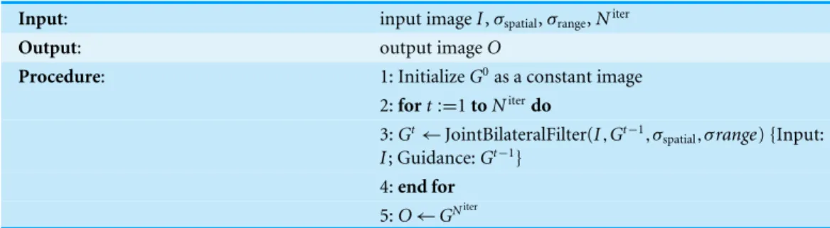
Table 1 Rolling Guidance Filter (RGF) algorithm (fromZhang et al.(2014)).
Input: input imageI,σspatial,σrange,Niter
Output: output imageO
Procedure: 1: InitializeG0as a constant image 2:fort:=1toNiterdo
3:Gt←JointBilateralFilter(I,Gt−1,σ
spatial,σrange) {Input:
I; Guidance:Gt−1} 4:end for
5:O←GNiter
increasing weights. Hence, guided by the input imageI, the RGF scheme gradually restores the edges that remain after the initial Gaussian filtering. Note that the initial guidance imageG1can simply be a constant (e.g., zero) valued image since it updates to the Gaussian filtered input image in the first iteration step. The pseudocode for the RGF scheme is presented inTable 1.
The RGF scheme is not restricted to the JBF (Zhang et al.,2014). Any average-based joint edge aware averaging filter (e.g., the Guided Filter) can be applied in the RGF framework. In practice the RGF converges rapidly after only a few (3–5) iterations steps. The RGF scheme is simple to implement and can be efficiently computed.
Although the RGF enables effective and efficient size selective filtering, it has as drawback that the remaining large scale edges are smoothly curved.
Smooth and iteratively Restore filter
Kniefacz & Kropatsch(2015) recently introduced the Smooth and iteratively Restore (SiR) filter. Similar to RGF, SiR initially removes small scale details (e.g., through Gaussian filtering) and uses an edge-aware filter to iteratively restore larger scale edges. Whereas RGF iteratively filters the (fixed) input image while iteratively restoring the initially blurred guidance image, SiR does the opposite: it gradually restores the initially blurred image using the original input image as (fixed) guidance. Thereto, small details are initially removed through blurring with a Gaussian kernel:
G0i =
1 K
X
j∈
Ij·f(ki−jk). (12)
Then, the edges of the remaining details are iteratively restored by repeatedly computing an updated imageGt+1by joint bilateral filtering of the blurred imageGt using the input
imageI as the guidance image:
Gti+1= 1
Ki X
j∈
Gtj·f(ki−jk)·g(kIi−Ijk). (13)
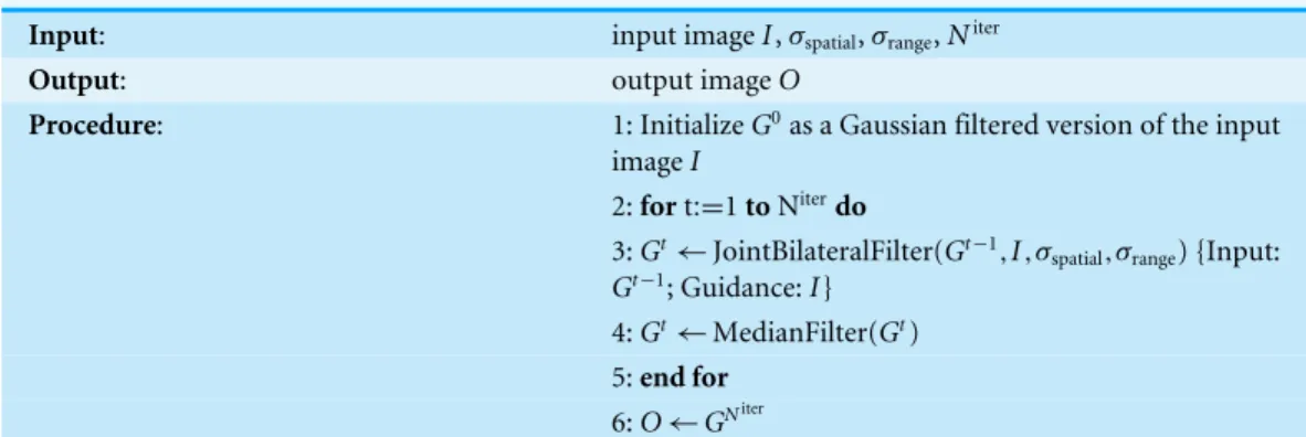
Table 2 Smooth and iteratively Restore with median filtering (SiRmed) algorithm (adapted from Kniefacz & Kropatsch(2015)).
Input: input imageI,σspatial,σrange,Niter
Output: output imageO
Procedure: 1: InitializeG0as a Gaussian filtered version of the input imageI
2:fort:=1toNiterdo
3:Gt←JointBilateralFilter(Gt−1,I,σ
spatial,σrange) {Input:
Gt−1; Guidance:I} 4:Gt←MedianFilter(Gt)
5:end for
6:O←GNiter
SiR also has two drawbacks (Kniefacz & Kropatsch,2015). First, the overall intensity of the result is less than the overall intensity of the original image, since SiR restores edges starting from the initially blurred input image. RGF does not have this problem because it operates on the original image itself. Second, SiR tends to restore small scale details that are close to large scale edges. This is a result of a spill-over effect (blurring) of the large scale edges which enables the JBF (Eq. (13)) to restore small scale details guided by the original input image. As will be shown in ‘Relative performance of SiR and SiRmed’ this restoration of small details near larger edges by SiR can effectively be suppressed by applying a median filter at the end of each iteration step with a kernel that is smaller than the Gaussian kernel of the bilateral spatial filter (e.g., 3×3). At each iteration step the median filer ‘‘cleans’’ the image by removing small details that are recovered by the bilateral filter. In the rest of this paper, we will refer to this modification of the original SiR algorithm as SiRmed (Smooth and iteratively Restore including median filtering). The pseudocode for the SiRmed algorithm is presented inTable 2. The pseudocode for the SiR algorithm is obtained by omitting Step 5 (the median filter).
ALTERNATING GUIDED FILTER
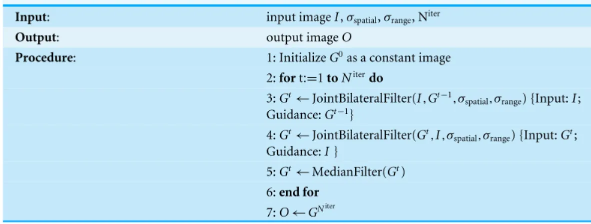
Table 3 Alternating Guided Filter (AGF) algorithm.
Input: input imageI,σspatial,σrange, Niter
Output: output imageO
Procedure: 1: InitializeG0as a constant image 2:fort:=1toNiterdo
3:Gt←JointBilateralFilter(I,Gt−1,σ
spatial,σrange) {Input:I; Guidance:Gt−1}
4:Gt←JointBilateralFilter(Gt,I,σ
spatial,σrange) {Input:Gt; Guidance:I}
5:Gt←MedianFilter(Gt)
6:end for
7:O←GNiter
prevents the reintroduction of filtered small scale details near large scale edges (a negative side effect of SiR). Hence, the AGF scheme combines the positive effects of both the RGF (intensity preservation) and SiR (edge curvature preservation) while eliminating their negative side effects (edge curvature smoothing by the RGF scheme and contrast reduction plus the reintroduction of small details near larger edges by the SiR scheme). The pseudo code for the AGF scheme is presented inTable 3.
EXPERIMENTAL RESULTS
In this section we present the results of some experiments that were performed to study the performance of the proposed AGF framework. We tested AGF by applying it to a wide range of different natural images (for an overview of all results see theSupplemental Informationwith this paper). Also, we compare the performance of AGF with that of RGF and SiRmed.
The images used in this study have a width of 638 pixels, and a height that varies between 337 and 894 pixels. We selected a set of test images with widely varying features and statistics, such as landscapes and aerial images, portraits and mosaics, embroidery and patchwork. The full set of test images with the results of the different filter schemes are provided asSupplemental Information.
In this study, color images are processed by applying the different algorithms to each channel in RGB color space independently. This was done to enable straightforward comparison with the results from previous studies (Kniefacz & Kropatsch,2015;Zhang et al.,2014). Note that in practical applications, filtering should preferably be performed in the CIE-Lab color space, so that only perceptually similar colors are averaged and only perceptually significant edges are preserved.
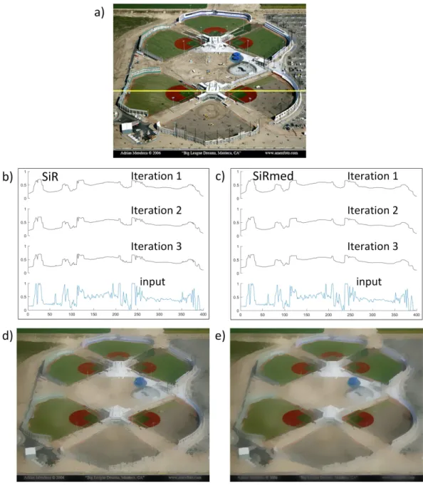
Figure 1 Effects of SiR and SiRmed filtering on image intensity.(A) Input image (Photo credit: Adrian Mendoza). (B, C) 1D Image intensity distribution along a horizontal cross section of (A) (yellow line) after the first 3 iterations of respectively SiR and SiRmed. The lowest curves show the original intensity distribution in (A). (D, E) Results after 5 iterations of respectively SiR and SiRmed. The spatial and range kernels used in the bilateral filters for this example were respectivelyσspatial=5 andσrange=0.05.
determined and resulted in an effective performance for all three frameworks on the entire set of selected test images.
Relative performance of SiR and SiRmed
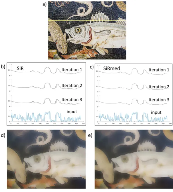
Figure 2 Effects of SiR and SiRmed filtering on image intensity.(A) Input image. (B, C) 1D Image in-tensity distribution along a horizontal cross section of (A) (yellow line) after the first 3 iterations of re-spectively SiR and SiRmed. The lowest curves show the original intensity distribution in (A). (D, E) Re-sults after 5 iterations of respectively SiR and SiRmed. The spatial and range kernels used in the bilateral filters for this example were respectivelyσspatial=5 andσrange=0.05.
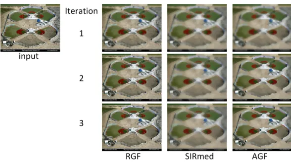
Figure 3 Results of RGF, SiRmed and AGF filtering for the first 3 iteration steps.The spatial and range kernels used in the bilateral filters for this example were respectivelyσspatial =5 andσrange=0.05. left. (Photo credit: Adrian Mendoza).
shows that SiR indeed restores high frequency details near large edge discontinuities, while SiRmed restores these large scale edges without the reintroduction of small scale details. This effect is also clearly demonstrated inFig. 2, where SiR fails to remove the small scale details all around the outlines of the tentacles and the fishes, while SiRmed effectively filters small elements all around these larger objects while both preserving their outlines and smoothing their interior.
Relative performance of RGF, SiRmed and AGF
Figure 3shows the results of RGF, SiRmed and AGF filtering after the first 3 iteration steps. Notice that all three filter schemes iteratively restore large scale image edges proceeding from an initial low resolution version of the input image. In this process RGF gradually smoothes the curvature of the large scale edges, while SiRmed smoothes the overall image intensity resulting in a global contrast reduction. In contrast, AGF restores the large scale edges without smoothing their curvature and with preservation of local image contrast.
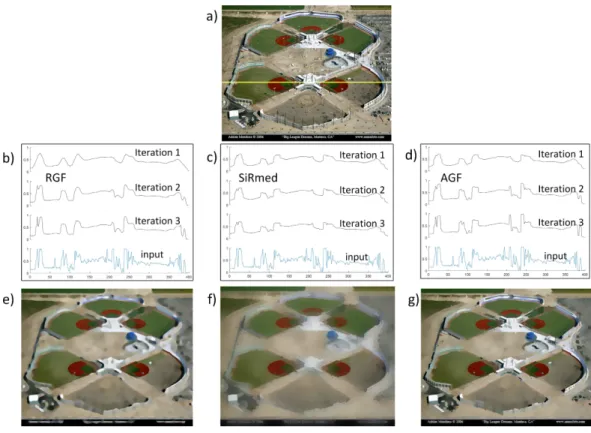
Figures 4B–4Dillustrate these effects by showing 1D horizontal cross sections. The contrast reducing effect of SiR is clearly shown inFig. 4Cas an overall reduction of the height of the large scale peaks. Comparison of Figs. 4Eand4Gillustrates that RGF smoothes the curvature of large scale edges while AGF preserves edge curvature.
Figure 4 Comparison of RGF, SiRmed and AGF filtering.(A) Input image (Photo credit: Adrian Men-doza). (B–D) 1D Image intensity distribution along a horizontal cross section (yellow line in (A)) after 3 successive iterations. (E–G) Results after 5 iteration steps. The spatial and range kernels used in the bilat-eral filters for this example were respectivelyσspatial=5 andσrange=0.05.
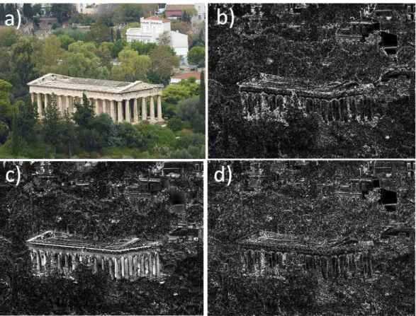
details all over the image support, while the original large scale edges (e.g., the outlines of the temple) remain relatively unaffected. In contrast, both RGF and SiRmed significantly alter the articulation of the original large scale edges. RGF smoothes the local edge curvature while SiRmed affects the local mean image intensity (resulting in local contrast reduction). As a result, large scale image contours (e.g., the outlines of the temple) are clearly visible inFigs. 5Band5C, and much less pronounced inFig. 5D.
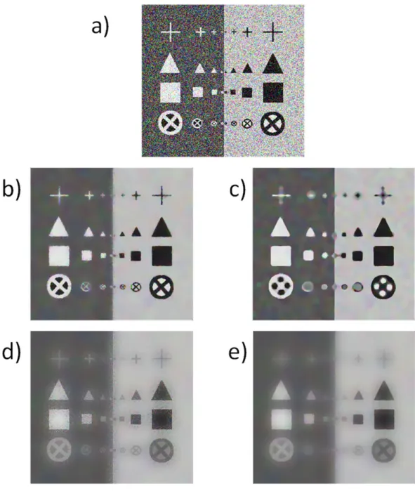
Figure 6further illustrates the differential performance of all four filters investigated here (AGF, RGF, SiR, and SiRmed) on an artificial image with noise.Figure 6A shows some simple geometric shapes (cross, triangle, square and wheel) with different sizes on a step-edge background with 30% additional Gaussian noise.Figures 6B–6Eshow the results of respectively AGF, RGF, SiR and SiRmed filtering ofFig. 6A after five iteration steps. This example shows that SiR restores noise near the edges of larger details and along the vertical step edge in the background, while AGF, RGF and SiRmed effectively reduce noise all over the image plane. Also, RGF (Fig. 6C) smoothes edge curvature, in contrast to AGF, SiR and SiRmed which retain the original edge curvature. This can for instance be seen in
Figure 5 The elimination of small scale details by RGF, SiRmed and AGF filtering.Absolute difference between input image (A) and the results of respectively RGF (B), SiRmed (C) and AGF (D) after 5 itera-tions. The images have been enhanced for visual display. The spatial and range kernels used in the bilateral filters for this example were respectivelyσspatial=5 andσrange=0.05.
intensity smoothing that is inherent in this method. AGF does not introduce any halos. In contrast, RGF produces high intensity halos, and SiR and SiRmed both produce halos with a large spatial extent (seeFig. 6Cnear the crosses and wheels).
Effects of different parameter settings
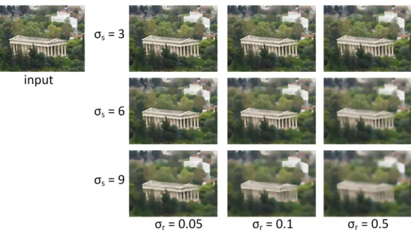
The results of RGF, SiRmed and AGF for different values of the parameters σs andσr
are shown inFigs. 7–9. In these figures rows correspond to different amounts of domain filtering (i.e., different values of σs) and columns to different amounts of range filtering (i.e., different values ofσr). These figures show that large spatial kernels and large range kernels both result in blurred image representations. Large spatial kernels cause averaging over large image areas, while large range kernels cause averaging over a wider range of image values.
In RGF (Fig. 7) the smoothing of large scale edge curvature increases with increasing
σs. This effect can for instance clearly be seen in the first column ofFig. 7(forσr=0.05) where the curves in the roof of the temple just above the pillars are still visible forσs=3, reduced forσs=6 and removed forσs=9.
Figure 6 Comparison of AGF, RGF, SiR and SiRmed filtering.(A) Artificial input image with 30% Gaussian noise added. Results of (B) AGF, (C) RGF, (D) SiR and (E) SiRmed filtering after 5 iteration steps. The spatial and range kernels used in the bilateral filters for this example were respectivelyσspatial=5 andσrange=0.05.
the contrast in the background vegetation around the temple is still visible for σs=3, reduced forσs=6 and almost removed forσs=9.
Figure 7 The effects of different parameter settings on RGF filtering.Results of RGF filtering of the in-put image for different values of the variances of the spatial (σs=3, 6 and 9) and range (σr=0.05, 0.1 and
0.5) filters.
Figure 8 The effects of different parameter settings on SiRmed filtering.Results of SiRmed filtering of the input image for different values of the variances of the spatial (σs=3, 6 and 9) and range (σr =0.05, 0.1 and 0.5) filters.
Runtime evaluation
Figure 9 The effects of different parameter settings on AGF filtering.Results of AGF filtering of the in-put image for different values of the variances of the spatial (σs=3, 6 and 9) and range (σr=0.05, 0.1 and
0.5) filters.
made no effort to optimize the code of the algorithms. We conducted a runtime test on a Dell Latitude laptop with an Intel i5 2 GHz CPU and 8 GB memory. The algorithms were implemented in Matlab 2016a. Only a single thread was used without involving any SIMD instructions. For this test we used a set of 22 natural RGB images (also provided in theSupplemental Informationwith this paper). The spatial and range kernels used in the bilateral filters for this test were fixed at respectivelyσspatial=5 andσrange=0.05, and the number of iterations was set to 5. The mean runtimes for AGF, RGF, SiR and SiRmed were respectively 3.80±0.27, 1.64±0.12, 1.80±0.14 and 2.17±0.16 s. This shows that the mean runtime of AGF is about equal to the sum of the runtimes of RGF and SiRmed. This result is as expected, since the steps involved in AGF are a combination of the steps involved in both RGF and SiRmed.
CONCLUSIONS
instance detail enhancement, denoising, edge extraction, JPEG artifact removal, multi-scale structure decomposition, saliency detection etc. (see e.g.,He, Sun & Tang,2013;Kniefacz & Kropatsch,2015;Zhang et al.,2014).
ADDITIONAL INFORMATION AND DECLARATIONS
Funding
This work was supported by the Air Force Office of Scientific Research, Air Force Material Command, USAF, under grant number FA9550-15-1-0433. The funders had no role in study design, data collection and analysis, decision to publish, or preparation of the manuscript.
Grant Disclosures
The following grant information was disclosed by the author:
Air Force Office of Scientific Research, Air Force Material Command, USAF: FA9550-15-1-0433.
Competing Interests
The author declares there are no competing interests.
Author Contributions
• Alexander Toet conceived and designed the experiments, performed the experiments, analyzed the data, contributed reagents/materials/analysis tools, wrote the paper, prepared figures and/or tables, performed the computation work, reviewed drafts of the paper.
Data Availability
The following information was supplied regarding data availability: The raw data has been supplied asSupplemental Dataset.
Supplemental Information
Supplemental information for this article can be found online athttp://dx.doi.org/10.7717/ peerj-cs.72#supplemental-information.
REFERENCES
Black MJ, Sapiro G, Marimont DH, Heeger D. 1998.Robust anisotropic diffusion.IEEE Transactions on Image Processing 7(3):421–432 DOI 10.1109/83.661192.
Farbman Z, Fattal R, Lischinski D, Szeliski R. 2008.Edge-preserving decompositions for multi-scale tone and detail manipulation.ACM Transactions on Graphics
27(3): Article 67DOI 10.1145/1360612.1360666.
He K, Sun J, Tang X. 2013.Guided image filtering.IEEE Transactions on Pattern Analysis and Machine Intelligence35(6):1397–1409DOI 10.1109/TPAMI.2012.213.
of the 39th annual workshop of the Austrian association for pattern recognition (OAGM2015). 1–9. eprint arXiv:1505.06702.
Paris S, Durand F. 2006. A fast approximation of the bilateral filter using a signal processing approach. In: Leonardis A, Bischof H, Pinz A, eds.Proceedings of the 9th European conference on computer vision (ECCV 2006), part IV. Berlin, Heidelberg: Springer Berlin Heidelberg, 568–580.
Perona P, Malik J. 1990.Scale-space and edge detection using anisotropic diffusion. IEEE Transactions on Pattern Analysis and Machine Intelligence12(7):629–639
DOI 10.1109/34.56205.
Petschnigg G, Agrawala M, Hoppe H, Szeliski R, Cohen M, Toyama K. 2004.Digital photography with flash and no-flash image pairs. In:ACM transactions on graphics (proceedings of SIGGRAPH2004). New York: ACM Press, 664–672.
Tomasi C, Manduchi R. 1998.Bilateral filtering for gray and color images. In:Proceedings of the IEEE sixth international conference on computer vision. Piscataway: IEEE, 839–846.