Revista Brasileira de Ensino de F´ısica,v. 35, n. 3, 3702 (2013) www.sbfisica.org.br
Lissajous-like figures with triangular and square waves
(Generaliza¸c˜ao de figuras de Lissajous com ondas triangulares e quadradas)J. Flemming
1, A. Hornes
Departamento de F´ısica, Universidade Estadual de Ponta Grossa, Ponta Grossa, PR, Brasil Recebido em 6/9/2012; Aceito em 1/4/2013; Publicado em 9/9/2013
We show a generalization of the well-known Lissajous figures, changing the two orthogonal simple harmonic oscillations to triangular and square-wave-type oscillations. All figures cross the origin of axes when there is no phase difference between the oscillations. Aside from this common feature, square-wave-type figures show a very different behavior, with discontinuous phase changes and impossibility of using a simple formula to get the frequency ratio between the two component oscillations.
Keywords: Lissajous figures, triangular and square waves, Fourier analysis.
Mostramos uma generaliza¸c˜ao das bem conhecidas figuras de Lissajous, trocando-se as duas oscila¸c˜oes harmˆonicas simples ortogonais por oscila¸c˜oes tipo onda triangular e onda quadrada. Todas as figuras cruzam a origem dos eixos quando n˜ao existe diferen¸ca de fase entre as oscila¸c˜oes. Excetuando-se esta caracter´ıstica em comum, as figuras formadas com ondas quadradas mostram um comportamento bastante distinto, com mudan¸cas descont´ınuas destas figuras conforme se varia a fase e a impossibilidade de utilizar uma f´ormula simples para obter a raz˜ao entre as frequˆencias das componentes oscilat´orias.
Palavras-chave: figuras de Lissajous, ondas triangulares e quadradas, an´alise de Fourier.
1.
Introduction
Lissajous figures are formed when two simple harmonic vibrations are coupled at right angle to each other [1]. Nathaniel Bowditch seems to have been the first (1815) to discuss such curves and Jules Antoine Lissajous stud-ied them on a deeper level in 1857-58 [2]. Besides their aesthetic beauty, Lissajous figures are used in under-graduate teaching laboratories to obtain the frequency of a signal (like sound, radio waves, etc.) by com-bining them with another signal of known frequency. Also, from the eccentricity of an ellipse (a typical Lis-sajous figure), one can precisely measure the phase dif-ference between two waves of the same frequency. Using this technique the speed of sound or light may be ob-tained by studying the phase difference between a direct modulated signal and another one which has traveled a precise distance [3, 4] or measure phase delays be-tween currents and voltages among components on an RLC circuit [5]. There are also recent research appli-cations of Lissajous figures as, for instance, commensu-rateness and phase between quantities relevant to he-licopter flight [6], light polarization structures created by using second-harmonic generation from lasers [7], Michelson interferometry to measure micro-vibration
displacements [8], oscillatory deformation in strongly nonlinear materials [9] and satellite trajectories around Lagrange points in the outer space [10].
Harmonic vibrations are the most usual scenario but triangular and square wave functions are also important periodic functions that one may come across. They are useful in digital circuits and frequency and time-interval measurements [11], besides other situations [12, 13]. Here we show what happens when one combines two orthogonal vibrations of these two latter types. These important cases seem to be left untouched, although some other variations of Lissajous figures have already been studied [14].
2.
Simulation and discussion
One may use several graphical software to trace those curves or, alternatively, an oscilloscope inX−Y mode
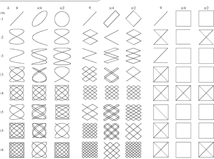
and two function generators. The results, illustrated in Fig. 1, were obtained with “Curvay” software [15] and were named Lissajous-like figures. Some true Lis-sajous curves, with harmonic vibrations, are shown in the first three columns (from left to right) of Fig. 1. They obey simple parametric equations, with timetas a parameter [1, 14]
1E-mail: [email protected].
3702-2 Flemming and Hornes
X = cos (ω1t− α), (1)
Y = cos(ω2t−β), (2)
where ω1/ω2 must be a rational number. For the sake of simplicity, we supposed unitary amplitudes for both vibrations. Several examples are shown, with variations of ratio between the two angular frequenciesω1/ω2and their phase difference δ = α– β, as indicated respec-tively on the left and upper side of Fig. 1.
Combinations of two orthogonal triangular and square-type vibrations are shown in the last six columns (from left to right) of the same figure, for phase dif-ferences of zero, π/4 and π/2. The curves for phase differences of 3π/4 and π (not shown) are symmetric and produce the same graphs as those ofπ/4 and zero respectively, except for a reflection about the vertical axis. For true Lissajous figures the ratio between the two frequencies is equal to the ratio of maximum
inter-sections of a vertical line and a horizontal one with the figure. In other words we have
fx fy
=Ny Nx
, (3)
wheref is the frequency in each axis andN the maxi-mum number of intersections of the true Lissajous fig-ure with a straight line parallel to the respective axis. For instance, in the fourth row of Fig. 1 the vertical fre-quency is 2/3 times the horizontal one, because one has vertical to horizontal intersections on the ratio 3/2 (for any phase difference). This basic feature of the true Lissajous figures also appears in the triangular case, which can be checked through the same example. So, for the triangular case, we may apply the same simple formula above to calculate the frequency in one axis if one knows the frequency in the other axis. On the other hand, this rule does not apply for the square Lissajous-like figures, as one can easily verify through the same example.
⌋
Lissajous-like figures with triangular and square waves 3702-3
Another interesting point to mention is the lack of continuity of the square Lissajous-like figures as a func-tion of the phase difference between components. For example, in the harmonic case with equal frequencies, one has a continuous change from a straight line seg-ment forδ= 0 to a circle forδ=π/2, through ellipses of different eccentricities. Something similar is valid for the triangular case. On the other hand, for the square type, we have a straight line segment forδ= 0 and then an abrupt change to a square figure with an infinites-imal δ increase. This square remains immutable until δ = π is reached, when it changes again abruptly to a straight line segment (oriented perpendicular to the first one). It is easy to see that this behavior comes from the fact that the square wave is a discontinuous function. For any frequency ratio, true Lissajous curves always pass through the origin of theX−Y plane when
δ= 0, which means no phase difference between the two harmonic waves [16]. As one can check by the examples in Fig. 1, this is a common characteristic also shared by the other two types of Lissajous-like figures studied here.
All periodic functions, as the square and triangu-lar waves, can be written as a Fourier series. One may argue, on such basis, that it is a straightforward math-ematical procedure to outguess the Lissajous-like fig-ures reported here and computer simulations are need-less. Although one can use Lissajous figures to Fourier analyze a given signal [17] the other way around (use Fourier analysis to forecast Lissajous-like figures) is not as easy. To see this let us expand, for instance, the square wave in Fourier series. If the wave has angular frequencyωand unitary amplitude, we have the follow-ing expression [18]
f(t) = 4 π
∞ ∑
n odd 1
nsinnωt. (4)
Suppose we combine two square waves with angular frequenciesω1andω2at right angle to each other, with unitary amplitudes and no phase difference between them. To forecast the Lissajous-like figure that would emerge from that, assume we truncate the Fourier ex-pansion at the pth term, for both waves. One must, then, sum up graphicallyp2true Lissajous figures, com-ing from the combinations of each term from one se-ries with each term of the other. As the square wave shows discontinuity points, the series above is not uni-formly convergent and one needs several terms to get a good approximation of the function, something known as the Gibb’s phenomenon [18]. If there is a phase dif-ference between the two square waves the situation is even worst, due to the greater number of variables in-volved. Of course, except for the Gibb’s phenomenon, the same arguments would apply for the construction of the Lissajous-like figures with triangular waves. Prelim-inary results from this manuscript were reported
else-where [19].
3.
Conclusions
In summary, we show what happens when one cou-ples two triangular or square waves at right angle to each other. These are important periodic functions, along with the harmonic case. We get the formation of what we named Lissajous-like figures, due to their resemblance to true Lissajous figures, formed with har-monic waves. Some aspects are common to all three types of figures, such as the origin crossing when there is no phase difference between the two orthogonal waves. Other features, as the possibility of calculating the fre-quency ratio between the waves by manipulating the figure, are not shared by the square-wave case. We generated these curves through graphical software. The need for simulations (or, alternatively, the use of an os-cilloscope) is justified from the fact that an algebraic Fourier forecast of these Lissajous-like figures is not a straightforward task. One may choose the particular free graphical software used here or different widespread options available nowadays, in order to easily reproduce these figures and introduce them in teaching laborato-ries.
References
[1] J.B. Marion and S.T. Thornton,Classical Dynamics of Particles and Systems(Harcourt, Forth Worth, 1988), 3rd
ed.
[2] Encyclopædia Britannica, “Curves, Special” (Ency-clopædia Britannica Inc., London, 1953), 14th
ed. [3] R.E. Berg and D.R. Brill, Phys. Teach.43, 36 (2005). [4] “Measurement of the Speed of Light” http:
//uni-leipzig.de/~prakphys/pdf/VersucheIPSP/ Optics/O-14e-AUF.pdf, access in March, 2013. [5] Phase Displacement in AC Circuits” http:
//uni-leipzig.de/~prakphys/pdf/VersucheIPSP/ Electricity/E-11e-AUF.pdf, access in March, 2013. [6] N. Sarigulklijn and M.M. Sarigulklijn, J. Aircraft34,
20 (1997).
[7] D.A. Kessler and I. Freund, Opt. Lett.28, 111 (2003). [8] Z.J. Li, S.L. Zhen, B. Chen, M. Li, R.Z. Liu and B.L.
Yu, Opt. Comm.281, 4744 (2008).
[9] R.H. Ewoldt and G.H. Mckinley, Rheol. Acta49, 213 (2010).
[10] D. Romagnoli and C. Circi, Celestial Mech. Dyn. As-tron.107, 409 (2010).
[11] P. Horowitz and W. Hill,The Art of Electronics (Cam-bridge University Press, Cam(Cam-bridge, 1989).
[12] S.M. Morgan and R.H. Victora, Appl. Phys. Lett.97, 093705:1 (2010).
[13] K. Miyasato, S. Abe, H. Takezoe, A. Fukuda and E. Kuze, Jap. J. Appl. Phys.22, L661 (1983).
3702-4 Flemming and Hornes
[15] “Curvay” software can be downloaded for free at http://www.spelunkcomputing.com/curvay/ download.html, access in March, 2013.
[16] M.S. Wu and W.H. Tsai, Am. J. Phys.52, 657 (1984). [17] P.P. Ong and S. H. Tang, Am. J. Phys.53, 252 (1985).
[18] P.H. Hwei, Fourier Analysis (Simon & Schuster, New York, 1967).