Core Inflation Measures for Brazil
Eurilton Araújo Ibmec São Paulo
Antonio Fiorencio Faculdades Ibmec/RJ and UFF
RESUMO
O presente artigo analisa as propriedades de duas medidas clássicas para o núcleo de in-flação, a saber: o estimador de média truncada e a medida baseada num VAR estrutural. O artigo também investiga uma pequena modificação na definição do estimador de média truncada, potencialmente capaz de melhorar sua capacidade de filtrar ruídos de alta freqüência. As medidas baseadas em média truncada são bastante similares e funcionam como uma aproximação imperfeita para um filtro passa baixa, capturando muito bem a tendência de longo prazo para a inflação. A medida baseada num VAR estrutural é bastante diferente das demais, enfatizando as freqüências médias relativamente às baixas freqüên-cias. Isto indica que flutuações cíclicas da inflação associadas a pressões de demanda são bastante importantes no médio prazo.
PALAVRAS-CHAVE
núcleo de inflação, domínio da freqüência, estimador de média truncada, VAR estrutural
ABSTRACT
This paper analyses the frequency domain properties of two well-known measures of core in-flation: the trimmed mean estimator and the SVAR estimator. It also investigates whether a small modification of the trimmed mean estimator enhances its capacity of filtering high-fre-quency noise. We find that the two versions of the trimmed estimator are rather similar. They work as imperfect approximations for low pass filters. Therefore, they are capturing very well trend inflation. The SVAR estimator, however, is quite different from both of them. It emphasizes intermediate frequencies rather than low frequencies, indicating that cyclical movements associated with excess demand pressures are very important in the medium run.
KEY WORDS
core inflation, frequency domain, trimmed estimator, SVAR
JEL Classification
INTRODUCTION
In recent years many central banks adopted inflation targets as a framework to the conduct of monetary policy. It is critical for these central banks to continuously evaluate inflationary trends to set monetary policy appropri-ately.
The trimmed estimator of core inflation is widely regarded as a useful indi-cator of “underlying inflation”.1 The rationale for the use of trimmed esti-mators of core inflation is by now well known. Price indexes are an average of individual prices. The arithmetic mean of observed prices is an efficient estimator of the general price level if the distribution of prices at a given moment is normal. But the international evidence suggests that the cross-sectional distribution of prices is leptokurtic and asymmetric. In fact, asym-metry is a strong feature of IPCA data, as suggested by Figueiredo (2001). These characteristics make the trimmed mean a more efficient estimator of central position. Given that, an important question is ‘How much should we trim?’ The optimal degree of trimming is usually chosen by minimising the mean squared error from the trimmed mean to a centred moving aver-age of inflation.
But, even though trimmed estimators of core inflation have become quite popular, they have been criticised for lacking economic rationale.2 An alter-native approach points to the fact that central banks should be concerned with demand driven price movements and that is what core inflation should measure. The structural vector auto-regression (SVAR) approach uses eco-nomic theory to impose identification restrictions on a standard VAR mod-el. The main problem here, of course, is to find compelling and credible restrictions.
Quah and Vahey (1995) proposed a SVAR measure of core inflation, char-acterized by long run restrictions, which identifies the output neutral
com-1 BRYAN & CECCHETTI, and co-authors, suggested the trimmed estimator of core inflation in several papers – see References. ROGER (1998), BAKHSHI &YATES (1999) and WYNE (1999) review the main issues.
ponent of inflation over medium to long run as the relevant measure of core inflation.
The Quah and Vahey (1995) SVAR measure includes cyclical movements in inflation due to excess demand. However, the measure excludes the impact of supply shocks, which may have permanent effects on the price level but just temporary effect on the rate of inflation.
Let be the trend inflation, is a measure of excess demand pres-sure, is the medium run component of inflation due to excess de-mand pressure, is the medium run component not related to demand pressures and is the transitory component of inflation.
If inflation, denoted by , can be decomposed as follows , then the SVAR measure is given by .
On the other hand, trimmed mean estimators are built to track trend infla-tion . Since these measures are based upon the analysis of a cross section of individual prices, they will be just an approximation to , with an error that may include the component given by or at least a frac-tion of it.
In any circumstances, both methods should be able to filter away high fre-quency components of inflation denoted by .
We want to assess these two measures of core inflation from a policy-orient-ed point of view. A central bank would not want to change its policy stance in reaction to a shock that would fade away within its targeting horizon anyway. In other words, central banks must filter away high frequency infla-tion shocks to get a picture of a meaningful indicator for core inflainfla-tion. The relevant measure of core inflation is closely related to the length of the monetary policy-maker’s horizon. If the focus is on a medium-term horizon, in which excess demand pressures may be important, then Quah and Vahey (1995) measure is appropriate. By contrast, if the policy horizon is longer, the trimmed mean estimator will deliver a more meaningful indicator for core
in-LR t
π Xt−1
) (Xt−1 g
MR t
π~
t
v
t
π
t MR t t LR
t
t =π +g X − +π +v
π ( 1) ~
)
( −1
+ t LR
t g X
π
LR t
π
LR t
π
MR t t
X
g( −1)+π~
t
flation, since it will capture trend inflation, as long as it is a reliable approxi-mation for trend inflation. In other words, the measure based on trimmed means should not capture a significant fraction of .
The amount of cyclical movements in inflation captured by the trimmed mean estimator is a quantitative question that will be investigated in this paper.
We analyse the frequency domain properties of the trimmed estimator and of the SVAR estimator of core inflation. In particular, we want to check whether they filter away high frequency noise.
In addition, we investigate the following issues. First, we assess whether the trimmed mean estimator is capturing cyclical movements, by measuring how close the trimmed mean measure of core inflation is to conventional definitions for . Second, we evaluate the importance of in the context of the SVAR measure, by examining if the SVAR measure is giving high weights to medium term fluctuations in inflation.
We also suggest a minor modification of the trimmed estimator that might enhance its capacity of filtering high frequency noise. Specifically, we con-struct our alternative proxy by applying a 1-year low-pass filter to the infla-tion series, instead of applying a moving-average filter.
We find that the core measures based on trimmed means work as approxi-mate low pass filter, emphasizing the long run component of inflation. On the other hand, the core based upon the bivariate SVAR specification tends to give weight to medium run components of inflation, reflecting the effect of demand shocks.
This paper is organized as follows. Section 1 presents the data we use. Sec-tion 2 analyses the frequency domain properties of the two alternative trimmed mean estimators of core inflation. Section 3 analyses the SVAR es-timator. Last Section offers conclusions.
MR t t
X
g( −1)+π~
LR t
1. THE INFLATION DATA
1.1 Basic Features
The data for inflation are the monthly percentage changes of IPCA at the item level of aggregation.3 The data for activity is the level of industrial pro-duction.4 All data are for the period 8/94-6/02.5
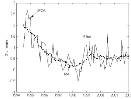
Figure 1 plots the IPCA6 series (continuous line).
FIGURE 1 - INFLATION
3 IPCA is the Extended Consumer Price Index computed by IBGE – Brazilian Institute of Geog-raphy and Statistics, a governmental agency. It is a weighted average of equivalent indexes for nine metropolitan areas and two municipalities. There were 47 items in the index until July 1999 and there 52 now.
4 The data for industrial production comes from IPEADATA, under the mnemonic ipeadata 1736265156, and the seasonality was already filtered.
5 In July 1994, Brazil launched the Real Plan and brought monthly inflation rates down from almost 50% to less than 1%. In January 1999, Brazil could no longer sustain its currency peg, it let the Real float and a few months later joined the group of countries adopting an inflation target framework for the conduct of monetary policy. At the time of writing, the Brazilian Central Bank (BCB) sets inflation targets for a horizon of about two and a half years. The tar-get is set for a headline consumer price index (IPCA) with a symmetric band and no escape clauses. In June 2002 the BCB altered the previously established target for 2003 and fixed the target for 2004.
Figure 2 shows that IPCA displays the positive skewness and the excess kur-tosis typical of this kind of data. Mean skewness and kurkur-tosis of IPCA are, respectively 0.76 and 10.0, and monthly variation is large.
FIGURE 2A - SKEWNESS
FIGURE 2B - KURTOSIS
1994 1995 1996 1997 1998 1999 2000 2001 2002 2003 -6
-4 -2 0 2 4 6 8
s
k
e
w
n
e
s
s
19940 1995 1996 1997 1998 1999 2000 2001 2002 2003 5
10 15 20 25 30 35 40
k
u
rt
o
s
1.2 Stationarity Issues
Before computing the two core inflation measures under study in this paper, we perform standard unit root tests for IPCA inflation. We first perform the Dickey and Pantula (1987) test in order to assess if the IPCA series is I (2). The test consists in a two step procedure. First, ADF regressions, employing the first difference of IPCA as the series to be tested, are used to test the null of two unit roots against the alternative of just one unit root. In the second step, the level of IPCA is used to test the null of one unit root against the alternative of none.
We choose the lag length in the ADF regressions using the AIC information criterion. We select the best specification for the deterministic component by looking at a measure of fit (the log-likelihood).
In order to get additional support concerning the stationarity nature of IPCA inflation, we perform two additional testing procedures, the Phillips-Perron and the KPSS tests for the presence of one unit root in the IPCA in-flation series.
Based on the results reported in Tables 1 to 3, unit root tests give mixed evi-dence concerning the existence of a unit root in IPCA inflation. Overall, tests indicate that inflation is stationary, but again this is not strongly sup-ported by all tests performed. For instance, allowing for a constant, which seems to be the best specification for IPCA inflation, based on the log-likeli-hood criterion, this series is stationary according to the ADF test, with lag length equal to 10, chosen by looking at the AIC criterion. Additionally, the first step in the Dickey and Pantula procedure did not give support to the hypothesis that the IPCA price index has two unit roots. The Phillips-Per-ron test supported the absence of a unit root for inflation. However, the KPSS LM statistics points to the rejection of the null, which in this case is absence of one unit root, since the best specification for the deterministic component seems to include constant and trend. In this case, as shown in Table 3, the test rejects the null of stationarity.
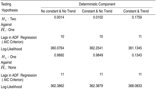
TABLE 1 – DICKEY & PANTULA ADF TEST FOR TWO UNIT ROOTS IN IPCA (p-values)
TABLE 2 – PHILLIPS & PERRON UNIT ROOT TEST FOR IPCA IN-FLATION (p-values)
TABLE 3 – KPSS UNIT ROOT TEST FOR IPCA INFLATION Testing Deterministic Component
Hypothesis No constant & No Trend Constant & No Trend Constant & Trend
Two Against
H1 : One
0.0014 0.0102 0.1759
Lags in ADF Regression ( AIC Criterion)
10 10 11
Log-Likelihood 360.0764 362.2541 361.1345
One Against
H1 : None
0.9892 0.9849 0.1343
Lags in ADF Regression ( AIC Criterion)
11 11 11
Log-Likelihood 362.3862 362.3879 368.0833
Testing Deterministic Component
Hypothesis No constant & No Trend Constant & No Trend Constant & Trend
One Against
H1 : None
0.0236 0.0169 0.0089
Log-Likelihood 373.0284 376.0853 378.0260
Testing Deterministic Component
Hypothesis Constant & No Trend Constant & Trend
None Against
H1 : One
Test Statistics 5% critical value Test Statistics 5% critical value
0.3832 0.463 0.1981 0.146
Log-Likelihood 338.0202 352.9024
:
0 H
:
0 H
:
0 H
:
1.3 Frequency Domain Properties
We now analyse the frequency domain properties of the inflation series. Any time series can be represented by its spectral density, which is given
by , where is the auto-covariance
function of order k and the letter i denotes the complex number unit. Th
e spectrum is just the Fourier Transform of auto-covariance
fun-ctions.
In the bivariate case, we have the cross-spectrum given by , where is the cross-covariance function of order k. The Greek letter denotes the angular frequency asso-ciated with cycles of periodicity given by . The spectrum and the cross-spectrum are estimated non-parametrically by Smoothing methods.7For instance, consider the univariate process . The sample periodogram, which is the sample analogue of , can be computed according to the following expression:
.
The symbol represents sample auto-covariance functions based on a sample of T observations, satisfying the condition for
A Kernel estimator averages the sample periodogram over different
frequen-cies and can be constructed as .
The Kernel assigns weights to each frequency considered.
Hamil-ton (1994) recommended the use of the Kernel .
7 For more details related to estimation procedures, see HAMILTON (1994).
{ }xt
∑
+∞ −∞ = − = k xx k i k
f ( )exp( )
2 1 )
( γ ω
π
ω γx(k)
∑
+∞ −∞ = − = k xyxy k i k
f ( )exp( )
2 1 )
( γ ω
π
ω γxy(k)
ω
ω π
2
{ }xt
) (ω x f ) exp( ) ( ˆ 2 1 ) ( ˆ 1 1 iwj j f T T j x
x =
∑
−− + − = γ π ω ) ( ˆx j
γ ) ( ˆ ) (
ˆx l γx j
γ = l =−j.
) ( ˆ ) ,
( j x j m
h h m m j f k + − = +
∑
ω ω ω) ,
( j m j
k ω + ω
2 ) 1 ( 1 ) , ( + − + = + h m h
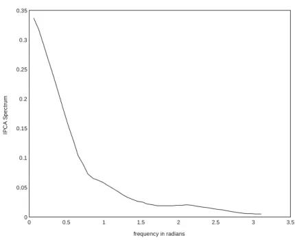
Figure 3 shows the power spectrum of IPCA. The spectrum was estimated using the recommended kernel with smoothing parameter h equal to 10. The spectrum shows the standard shape of the spectral density of a macro-economic time series, characterized by concentrating mass in the low fre-quency range. The decay pattern is not so fast though. Almost 70 per cent of the spectral mass is concentrated in the range defined by zero and 0.79 radians, which corresponds to cycles with periodicity of approximately more than eight months.
FIGURE 3 - POWER SPECTRUM
1.4 Measures of Long Run Inflation
In order to compute trimmed-mean measures of core inflation, it is neces-sary to have a measure of long run inflation to be used as benchmark in the construction of the core measure. We present two alternative measures of long run inflation, which are going to be used in the rest of the paper. To eliminate the high-frequency components of IPCA and get a measure of long run inflation, we apply to it a 1-year low-pass filter. The low-pass-filter
0 0.5 1 1.5 2 2.5 3 3.5
0 0.05 0.1 0.15 0.2 0.25 0.3 0.35
frequency in radians
IP
C
A
S
pec
tr
is a special case of a band-pass-filter with the passing band defined from zero up to a specified frequency.
Generally, the Ideal Band Pass Filter is the artefact used to extract particular frequency components associated with a given series. The Ideal Band Pass Filter is just a linear transformation of the data, which does not change the data within a specified frequency band and eliminates all other frequency components.
A filtered series can be represented as follows, where the
poly-nomial is given by with the condition being
satisfied.
T
he Ideal Band Pass Filter, for the specified frequency band
, is an infinite moving average, characterized by a set of
weights, computed
according to the following expressions:and for
Therefore, to apply the Ideal Band Pass Filter, an infinite amount of data is needed. For this reason, some sort of approximation has to be used. Chris-tiano and Fitzgerald (2003) study optimal linear approximations to the un-achievable Ideal Band Pass Filter. They define weights for a linear combination involving all data points in the sample. Their recommended weights vary with the time index and are not symmetric. Therefore, one does not loose data points though the first year and last year of filtered data are poorly estimated.
Our low-pass-filter is built according to Christiano and Fitzgerald (2003) and we decide to discard the first six and last six values generated by their algorithm, since they are poorly estimated and the series length is the same
t F
t B L x
x = ( )
) (L
B h
h hL
b L
B ∑
+∞
−∞ =
=
)
( bh =b−h
] ,
[f1 f2
π
1 2 0
f f
b = −
h h f h
f bh
π
) sin( )
sin( 2 − 1
as the six-month centred moving average of IPCA, which facilitates com-parison. The filtered series is shown as the broken line in Figure 1.
Figure 1 also shows, as the dotted line, our second measure of long run in-flation, which is the six-month centred moving average of IPCA. The fact that moving averages tend to eliminate high frequency components is evi-dent in the figure. Though, the six-month moving average cannot filter away a one-year seasonal effect, choosing a twelve-month moving average as the benchmark series would leave us with very few data points to per-form computations in the frequency domain in a reliable way.
The next section shows results concerning an asymmetric trimmed mean measure of core inflation based upon the two measures of long run inflation just described above.
2. TRIMMED MEAN ESTIMATORS OF CORE IPCA8
2.1 Building Trimmed Mean Estimators
To facilitate comparison with other studies, we compute a simple measure of core inflation: an asymmetric trimmed (weighted) average of percentage changes in the prices of individual products. The degree of trimming is cho-sen to minimise the mean squared error of the trimmed estimator from a six-month centred moving average of IPCA.9 We call this estimator the MA-core. Since moving averages reduce high-frequency noise, the MA-core targets a measure of trend inflation.
We also compute an alternative measure of core inflation. We continue to use an asymmetric trimmed mean estimator, but we choose the degree of trimming by minimising the mean squared error from the trimmed
estima-8 Measures of core inflation for Brazil have been calculated by BRYAN & CECCHETTI (2001), FIORENCIO & MOREIRA (2000), FIGUEIREDO (2001), MOREIRA & MIGON (2001), PICCHETTI & KANCZUK (2001).
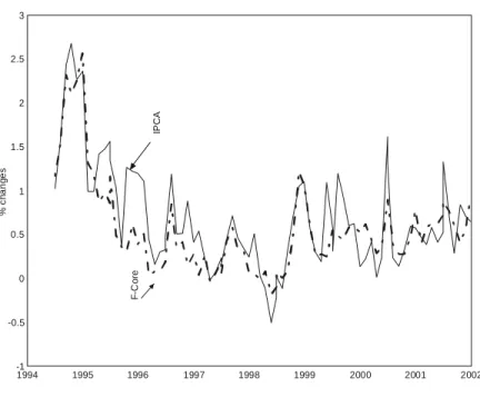
tor to a 1-year low-pass filtered IPCA. We call this estimator the F-core. The motivation for computing this alternative core is rather obvious. Since inflation targets are set for specific horizons, it is interesting to evaluate in-flation prospects at those frequencies. The low-pass filter allows a better def-inition of the frequencies of interest than does the MA filter.
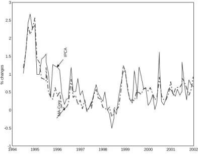
Figure 4 and Figure 5 show plots of the MA-core and of the F-core. The difference between the two core measures is hardly discernible. The optimal MA-core trims 20.15 % of the right tail and 17.28 % of the left tail, where-as the optimal F-core trims 19.94 % of the right tail and 16.78 % of the left tail. The optimal degrees of trimming are quite similar for both estimators. They remain similar when we change the window of the moving average and when we consider a symmetric trimming.
FIGURE 4 – INFLATION
10 The choice of 1-year for the cutting frequency is arbitrary. We have not yet experimented with other cutting frequencies for the low-pass filter but intend to do so.
1994 1995 1996 1997 1998 1999 2000 2001 2002
-1 -0.5 0 0.5 1 1.5 2 2.5 3
%
c
h
a
n
g
e
s
IP
C
A
MA
-C
o
FIGURE 5 – INFLATION
2.2 Frequency Domain Analysis
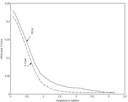
We now turn to the frequency domain properties of the two trimmed esti-mators of core inflation. Figure 6A shows the power spectrum of IPCA and of the MA-core. Figure 6B shows the power spectrum of IPCA and of the F-core.11 As is well known, the variance of a series is the area under its spec-trum. The figures show the expected reduction in the variance of the series produced by the two filters.
11 The two power spectra of IPCA are not identical because they were estimated on different data samples, since the MA-core loses 6 observations on each end of the sample.
1994 1995 1996 1997 1998 1999 2000 2001 2002 -1
-0.5 0 0.5 1 1.5 2 2.5 3
%
c
h
a
n
g
e
s
IP
C
A
F-C
o
FIGURE 6A – POWER SPECTRUM
FIGURE 6B – POWER SPECTRUM
0 0.5 1 1.5 2 2.5 3 3.5
0 0.05 0.1 0.15 0.2 0.25
frequency in radians
IP
C
A
an
d M
A
-C
or
e IPC
A
M
A
-C
or
e
0 0.5 1 1.5 2 2.5 3 3.5
0 0.05 0.1 0.15 0.2 0.25
frequency in radians
IP
C
A
a
n
d
F
-C
o
re
IP
C
A
F-C
o
Since we are interested in the relationship between alternative cores and IPCA inflation in the frequency domain, it is necessary to discuss a mathe-matical object, based on cross-spectrum that summarizes this relationship.
The relationship between the input series and the output series of a system is measured by the Transfer Function, which is defined by the ra-tio . As any complex number, the Transfer Function has a modulus, often called gain and an angle, usually known as phase.
We will show the Transfer Function gains considering IPCA inflation, as in-put series and the cores we intend to study, as outin-put series.
Figure 7A compares the transfer function gains of the MA-core with the transfer function of the moving average itself. Figure 7B does the same for the F-core and the low-pass filter. The figures show that both cores reduce high-frequency noise much less than their ideal counterparts.
FIGURE 7A – TRANSER. FUNCTION GAIN
{ }xt { }yt
) (
) (
ω ω
x xy
f f
0 0.5 1 1.5 2 2.5 3 3.5
0 0.1 0.2 0.3 0.4 0.5 0.6 0.7 0.8 0.9 1
frequency in radians
M
A
an
d
MA
-C
or
e
M
A
-C
o
re
FIGURE 7B - TRANSFER FUNCTION GAIN
The contribution of cycles associated with the frequency band to total variance is given by the following integral . All frequen-cies belong to the interval and stands for the spectrum of the series being studied.
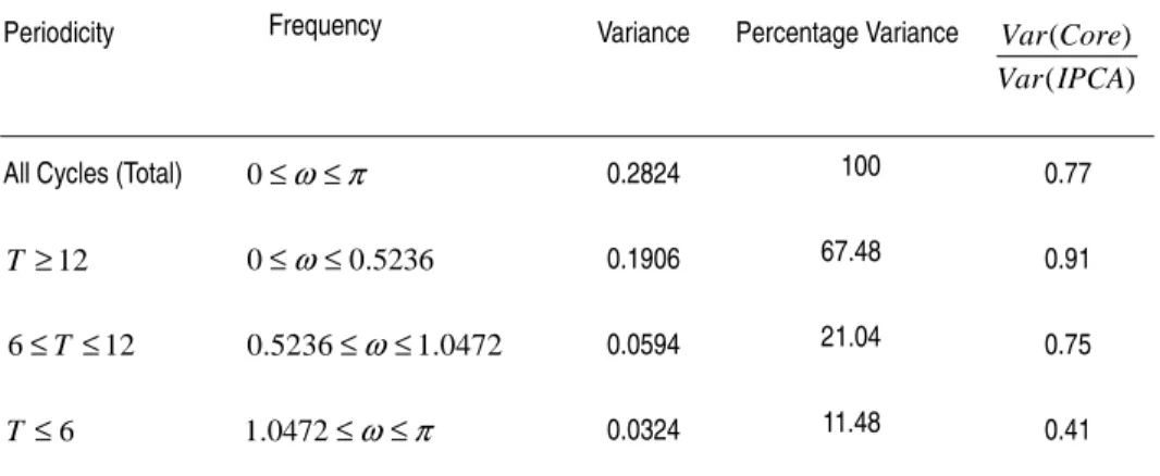
Tables 4, 5 and 6 assess quantitatively the contribution of different frequen-cy bands to total variance for IPCA inflation, MA-Core and F-Core.
TABLE 4 – IPCA INFLATION
Periodicity Frequency Variance Percentage of Variance
All Cycles (Total) 0.3664 100
0.2085 56.92
0.0795 21.70
0.0784 21.38
0 0.5 1 1.5 2 2.5 3 3.5
0 0.1 0.2 0.3 0.4 0.5 0.6 0.7 0.8 0.9 1
frequency in radians
Fi
lt
er
a
n
d
F
-C
o
re
F
-C
o
re
F
ilte
r
] ,
[ω1 ω2
∫
2 1) (
2 ω
ω fx ω dω
] , 0
[ π fx(ω)
π ω ≤ ≤
0
12
≥
T 0≤ω≤0.5236
12
6≤T≤ 0.5236≤ω≤1.0472
6
≤
TABLE 5 – MA CORE
TABLE 6 – F CORE
By comparing Table 4 and Table 5, it is clear that the MA-Core is able to re-duce total variance as well as the variance in each band of frequency analyzed. Most of the reduction in variance is associated with high frequen-cy components, which account for 11.1% of the variance in the core and is less than half the variance of high frequency components in the original IPCA series. The six to twelve month component is still as important as it is in the IPCA series, though its variance is lower than the variance of the same component in the original IPCA. Low frequency components are more important in the MA-Core, accounting for 68 % of the variance in the core. The reduction of variance associated with the long run (low frequenci-Periodicity Frequency Variance Percentage Variance
All Cycles (Total) 0.2884 100 0.79
0.1961 68.0 0.94
0.0603 20.9 0.76
0.0320 11.1 0.41
Periodicity Frequency Variance Percentage Variance
All Cycles (Total) 0.2824 100 0.77
0.1906 67.48 0.91
0.0594 21.04 0.75
0.0324 11.48 0.41
) (
) (
IPCA Var
Core Var
π ω≤ ≤
0
12
≥
T 0≤ω≤0.5236
12
6≤T≤ 0.5236≤ω≤1.0472
6
≤
T 1.0472≤ω≤π
) (
) (
IPCA Var
Core Var
π ω≤ ≤
0
12
≥
T 0≤ω≤0.5236
12
6≤T≤ 0.5236≤ω≤1.0472
6
≤
es) is small. In short, the MA-Core behaves like a low pass filter, emphasi-zing the long run.
By comparing Table 4, Table 5 and Table 6, one can see that the properties of the F- Core are the same as the MA-Core. In other words, we see a re-duction in variance in all frequencies band, but the rere-duction is much bigger in the high frequency range. In addition, long run components are empha-sized, since the concentration of variance in low frequencies, in percentage terms, has increased.
The main conclusion from this section is that using a low-pass filter or a moving-average to proxy for trend inflation produces similar cores. The op-timal degrees of trimming do not change much and the spectrum of the F-Core is not superior to the spectrum of the MA-F-Core, in the sense of having much less power at high frequencies. The MA-Core has the advantage of being simpler to compute. Of course, these are empirical results that may or may not apply to other data sets.
3. A SVAR CORE OF IPCA
3.1 Building the SVAR Measure
The SVAR methodology is based upon Quah and Vahey (1995). It amounts to an application of the Blanchard and Quah identification strategy to define a measure of the underlying inflation. Core Inflation is defined as the component of measured inflation that has no long-run effect on output. We call this estimator the S-core. Behind that definition is the idea that cen-tral bankers should be concerned only with inflation related to demand shocks.
Let us denote the growth of industrial production by and the inflation rate by . Consider the vector and the structural shocks and .
The reduced form VAR can be written as:
The VAR is estimated in its reduced form and is used to compute the re-siduals and .
The vector can be written in a moving average representation according to . The moving average representation associated with the
residuals is . The identity matrix is denoted by the letter
I. The Greek and denote vectors stacking structural shocks and
re-siduals respectively.
Comparing both moving average representations, it is not hard to show that the structural shocks and the residuals are related by the following equations:
Since the residuals are obtained via reduced form estimation, to recover the structural shocks one need to know the coefficients .
The variance-covariance matrix of residuals gives three conditions that are related to the variances of the two residuals and to the covariance between them. These conditions involve the four unknowns , two known variances and a known covariance. But we still have four unknowns and only three equations.
t
y
Δ
t
π xt =(Δyt πt)T ε1
2
ε
t t t
t A L y A L e
y = 11( )Δ 1+ 12( ) 1+ 1
Δ − π −
t t t
t = A21(L)Δy−1 +A22(L)π −1 +e2 π
1
e e2
t x
∑
∞ = − = 0 ) ( j j tt C j
x ε
∑
∞ = − + = 1 ) ( j j t t I B j ex
j t−
ε et−j
t t
t c c
e1 = 11(0)ε1 + 12(0)ε2
t t
t c c o
e2 = 21(0)ε2 + 22( )ε2
)} 0 (
{cij
)} 0 (
Using the Blanchard and Quah strategy for identification, one can impose a restriction that the long-run impact of one shock in one of the variables is zero. So, one can impose that the first shock will not have any effect on out-put in the long run. That restriction implies a fourth equation involving and and known quantities which came from the reduced form estimation.
The four equations just described are:
Finally, we will have four unknowns and also four equations. By solv-ing that system, one is able to find the matrix . Knowing the re-siduals and the inverse matrix of , it is straightforward to recover the structural shocks. After that step is completed, the process for in-flation can be written as a function of the structural shocks as follows
.
Here we are assuming that we are truncating the infinite moving average representation, using the same lag length employed in the estimation of the reduced form system. The SVAR measure of core inflation is .
) 0 (
11
c c21(0)
2 12 2 11
1) (0) (0)
(e c c
Var = +
2 22 2 21
2) (0) (0)
(e c c
Var = +
) 0 ( ) 0 ( ) 0 ( ) 0 ( ) ,
cov(e1 e2 =c11 c21 +c12 c22
∑
∑
= = + − = p k p k k a c k a c 0 12 21 0 2211(0)[1 ( )] (0)[ ( )]
0 ) 0 ( C ) 0 ( C
∑
∑
= − = − + = p j j t p j j tt c j c j
0
2 22 0
1
21( )ε ( )ε
3.2 Stationarity Issues and VAR Specification
3.2.1 Testing for Unit Roots in Industrial Production
Since we have already discussed stationarity properties concerning IPCA in-flation, we present unit root tests related only to the Industrial Production series. Tests gave strong support to the presence of a unit root in the indus-trial production series. For instance, applying the two step Dickey and Pan-tula (1987) test for the presence of two unit roots, the hypothesis that industrial production is I(2) was strongly rejected for all specifications re-lated to the deterministic component of the time series for industrial pro-duction. In the same vain, the ADF statistics gave support to the absence of a unit root for industrial production growth. In addition, Phillips-Perron and KPSS tests also supported the non-stationary nature of the index of in-dustrial production since they both have indicated that the growth of indus-trial production is not an integrated process of order one.
TABLE 7 – DICKEY & PANTULA ADF TEST FOR TWO UNIT ROOTS IN INDUSTRIAL PRODUCTION (p-values)
Testing Deterministic Component
Hypothesis No constant & No Trend
Constant & No Trend
Constant & Trend
Two Against
H1 : One
0.0000 0.0001 0.0000
Lags in ADF Regression (AIC Criterion)
0 0 0
Log-Likelihood 220.0391 220.3524 220.3608
One Against
H1 : None
0.8779 0.4503 0.3174
Lags in ADF Regression (AIC Criterion)
1 1 1
Log-Likelihood 220.3397 221.7478 223.5703
:
0 H
:
TABLE 8 – PHILLIPS & PERRON UNIT ROOT TEST FOR INDUSTRI-AL PRODUCTION GROWTH (p-values)
TABLE 9 – KPSS UNIT ROOT TEST FOR INDUSTRIAL PRODUCTION GROWTH
3.2.2 Specifying the VAR System
Using our data set, we estimate a VAR with lag length equal to six. We choose the lag length considering two criteria. The first one is the ability of the statistical model to fit the data parsimoniously. The second is the ab-sence of autocorrelation in the residuals, reflecting the fact that all the rele-vant information is captured by the model.
We start to search for an adequate specification for the VAR, initially, by comparing AIC and Schwartz criteria for various lag length going from two to eight. In order to minimize the information criteria, the best specification is a VAR (2). In spite of that, a very short VAR specification is not able to generate white-noise-like residuals, as shown in Table 11. It is necessary to
Testing Deterministic Component
Hypothesis No constant & No Trend
Constant & No Trend
Constant & Trend
One Against
H1 : None
0.0000 0.0001 0.0000
Log-Likelihood 220.0391 220.3524 220.3608
Testing Deterministic Component
Hypothesis Constant & No Trend Constant & Trend
Two Against
H1 : One
Test Statistics 5% critical value Test Statistics 5% critical value
0.0494 0.463 0.0472 0.146
Log-Likelihood 216.1534 216.1869
:
0 H
:
increase the lag length to eliminate autocorrelation in the residuals. So, ob-taining residuals that look like a white noise as much as possible is a much more important consideration than following the parsimonious specifica-tion suggested by the usual informaspecifica-tion criteria. Tables 12 and 13 summa-rize the estimated VAR.
TABLE 10 – LAG LENGTH CHOICE FOR THE VAR BASED ON IN-FORMATION CRITERIA
TABLE 11 – MULTIVARIATE LM TEST FOR AUTOCORRELATION (P-VALUES)
Lag AIC Schwartz
2 -3.6854 -3.3998
3 -3.6631 -3.2605
4 -3.5923 -3.0750
5 -3.6093 -2.9717
6 -3.6444 -2.8972
7 -3.5737 -2.7116
8 -3.5107 -2.5337
Lag VAR(2) VAR(4) VAR(6)
1 0.0013 0.0041 0.6695
2 0.0321 0.0043 0.4292
3 0.8277 0.2588 0.6711
6 0.0859 0.6032 0.1100
TABLE 12 – FIRST EQUATION: INDUSTRIAL PRODUCTION GROWTH IS THE DEPENDENT VARIABLE
TABLE 13 – SECOND EQUATION: IPCA INFLATION IS THE DE-PENDENT VARIABLE
Variable Coefficient t Statistics
Constant 0.004401 1.07992
IP Growth (-1) -0.361597 -3.18276
IP Growth (-2) 0.049629 0.43382
IP Growth (-3) 0.051546 0.44838
IP Growth (-4) 0.021803 0.19048
IP Growth (-5) -0.169934 -1.51854
IP Growth (-6) -0.123277 -1.17199
IPCA Inflation (-1) -0.001295 -0.19855
IPCA Inflation (-2) -0.003924 -0.51417
IPCA Inflation (-3) 0.013489 1.79814
IPCA Inflation (-4) -0.012895 -1.72948
IPCA Inflation (-5) 0.012448 1.69665
IPCA Inflation (-6) -0.012243 -2.04318
Variable Coefficient t Statistics
Constant 0.118146 1.65017
IP Growth (-1) -2.798083 -1.40194
IP Growth (-2) -4.255435 -2.11745
IP Growth (-3) -1.517366 -0.75133
IP Growth (-4) -0.590151 -0.29349
IP Growth (-5) -1.194244 -0.60748
IP Growth (-6) -0.270651 -0.14647
IPCA Inflation (-1) 0.644527 5.62570
IPCA Inflation (-2) -0.251644 -1.87709
IPCA Inflation (-3) 0.195367 1.48242
IPCA Inflation (-4) -0.147717 -1.12777
IPCA Inflation (-5) 0.182482 1.41577
We perform Normality test in the residuals and reject the null hypothesis of residuals following a Bivariate Normal distribution at 5 per cent, based on the p value of 0.025 for the Jarque-Bera test. Lack of residuals following a joint Normal distribution is not a major problem for the VAR(6) specified, since we are interested in using the VAR to build a measure of core inflation and do not use residuals to any sort of additional testing which demands Normality.
To gauge the adequacy of the VAR (6) in describing the joint process for industrial production and IPCA inflation, we simulate artificial time series for inflation and industrial production 1000 times and compute two stan-dard errors bands, shown in Figure 8. Most of the time, the observed time series for inflation and industrial production were inside the two standard errors bands. Therefore, the VAR (6) is a plausible representation for the joint process involving industrial production and IPCA inflation and can be used as raw material for building the measure of core inflation proposed by Quah and Vahey (1995).
FIGURE 8A – OBSERVED AND SIMULETED VALUES FROM VAR(6) -INFLATION
-1 0 1 2 3 4
1995 1996 1997 1998 1999 2000 2001
INFLAM+2SE INFLAM-2SE
FIGURE 8B – OBSERVED AND SIMULATED VALUES FROM VAR(6) - IND PROD
3.3 Results and Frequency Domain Analysis
Figure 9 shows that the S-core is able to track the observed IPCA well, es-pecially after the second half of 1995. Figure 10 shows the spectrum of the S-core12 and Figure 11 shows its transfer function, which is markedly differ-ent from the transfer functions of the MA-core and the F-core. We see that the S-core does not give a high gain to the low frequencies. This is not sur-prising since the S-core is not built to be close to any type of smoother. It is the middle frequencies that are being highlighted by the SVAR procedure.
12 The same comments concerning the change of scale in the spectrum of IPCA made with respect to Figure 6 apply here. The SVAR procedure implied a loss of 12 months of observations.
-.12 -.08 -.04 .00 .04 .08 .12
1995 1996 1997 1998 1999 2000 2001
Ind Prod(Observe Values) Ind ProdM+ 2SE Ind ProdM-2SE
FIGURE 9 – INFLATION
FIGURE 10 – POWER SPECTRUM
1995 1996 1997 1998 1999 2000 2001 2002 2003
-1 -0.5 0 0.5 1 1.5 2
%
c
h
a
n
g
e
s
IP
C
A
SV
A
R
C
o
re
0 0.5 1 1.5 2 2.5 3 3.5
0 0.01 0.02 0.03 0.04 0.05 0.06 0.07 0.08 0.09 0.1
frequency in radians
IP
C
A
a
n
d
S
V
A
R
C
o
re IPCA
SV
A
R
Cor
FIGURE 11 – TRANSFER FUNCTION GAIN
Tables 14 and 15 assess quantitatively the contribution of different frequen-cy bands to total variance for IPCA inflation and S-Core. Of course, we are taking into account that we lost 12 months of observations by estimating the SVAR Core. Therefore, we recomputed the figures for IPCA inflation in order to compare them with the ones related to the S-Core.
TABLE 14 – IPCA INFLATION
Periodicity Frequency Variance Percentage of Variance
All Cycles (Total)
0.2 100
0.0877 43.85
0.0451 22.54
0.0672 33.61
0 0.5 1 1.5 2 2.5 3 3.5
0.3 0.4 0.5 0.6 0.7 0.8 0.9 1
frequency in radians
S
V
A
R
C
o
re
π ω ≤ ≤
0
12
≥
T 0≤ω≤0.5236
12
6≤T≤ 0.5236≤ω≤1.0472
6
≤
TABLE 15 – S CORE
The tables show that the S-Core is capable of reducing the variance in all frequency bands analyzed. Though, in contrast to the MA and F-core, the reduction in volatility is small for components associated with high frequen-cy frequen-cycles. The overall reduction in variance is comparable with the reduction achieved by the trimmed mean based core measures. The difference is that low frequency components are not emphasized, since the aim of the SVAR based core measure is to identify demand driven movement in inflation. The ratio between the S-core and the original inflation series variances in the range of frequencies associated with periodicity of more than one year is lo-wer when compared to the cases of the MA-Core and F-Core.
In short, though the ratio between the S-core and the original inflation total variances are more or less the same for all measures of core studied (be-tween 0.7 and 0.8), the reduction in variance has a different pattern de-pending on the measure studied. The trimmed mean based measures achieve a reduction in total variance, based on a low variance reduction in low frequencies and a high variance reduction in high frequencies. The S-Core, by contrast, works in such a way that the medium run is more em-phasized then the long run.
CONCLUSIONS
Many central banks look at different measures of core inflation in order to define their policy stances. In this paper we performed an empirical evalua-tion of two popular measures of core inflaevalua-tion: two versions of the trimmed Periodicity Frequency Variance Percentage
Variance
All Cycles (Total) 0.1432 100 0.72
0.0467 32.64 0.53
0.0340 23.77 0.75
0.0625 43.59 0.93
) (
) (
IPCA Var
Core Var
π ω≤ ≤
0
12
≥
T 0≤ω≤0.5236
12
6≤T ≤ 0.5236≤ω≤1.0472
6
≤
mean estimator and the SVAR estimator of core inflation. Specifically, we investigated the frequency domain properties of these estimators.
We found that the differences between the two versions of the trimmed esti-mator are minor. The MA-core and the F-core series are similar and, natu-rally, so are their spectra and transfer functions. It will be interesting to test whether this similarity is dependent on the specific cutting frequency (1 year) that we arbitrarily chose. The MA-core has the advantage of being easier to compute. The F-core has the advantage of a greater precision in the definition of what is meant by “trend” inflation. This greater precision might be important if the similarity between the two estimators does de-pend on the chosen cutting frequency.
The differences between the two trimmed estimators and the SVAR estima-tor are considerable. The S-core aims at separating demand from supply shocks to inflation whereas the MA-core and the F-core aim at separating high frequency from low frequency movements. This difference in objec-tives translates clearly into differences on their frequency characteristics. The S-core highlights intermediate frequencies whereas the MA-core and the F-core emphasize low frequencies.
In short, the two trimmed estimators are reliable measures of trend inflation and the SVAR estimator attaches great importance to intermediate frequen-cies, showing that demand driven movements are very important for medi-um run fluctuations. Therefore, if the policy-maker’s horizon is a medimedi-um- medium-term horizon, then the SVAR measure is appropriate, since it is relating a significant part of medium run fluctuations to demand driven movements in inflation. On the contrary, if the policy-maker is solely concerned with the long run, she should adopt the trimmed mean measure of core inflation as the relevant target for the monetary policy.
REFERENCES
BRYAN, M. F.; CECCHETTI, S. G. The CPI as a measure of inflation.
Economic Review, Federal Reserve Bank of Cleveland, v. 29, n. 4, p. 15-24, 1993.
_______. Measuring core inflation. In: MANKIW, N. G. (ed.), Monetary policy. The University of Chicago Press, 1994.
_______. A note on the efficient estimation of inflation in Brazil. Central Bank of Brazil, Working Paper 11, 2001.
BRYAN, M. F.; CECCHETTI, S. G.; WIGGINS II, R. L. Efficient infla-tion estimainfla-tion. NBER Working Paper n. 6183, 1997.
CECCHETTI, S. G. Measuring short-run inflation for central bankers.
Economic Review, Federal Reserve Bank of Saint Louis, p. 143-155, May/June, 1997.
CECCHETTI, S. G.; GROSHEN, E. L. Understanding inflation: impli-cations for monetary policy. NBER Working Paper n. 7482, 2000. CHRISTIANO, L. J.; FITZGERALD, T. J. The band pass filter.
Interna-tional Economic Review, v. 44, n. 2, p. 435-466, 2003.
DICKEY, D. A.; PANTULA, S. G. Determining the order of differencing in autoregressive processes. Journal of Business and Economic Statis-tics, v. 5, n. 4, p. 455-461, 1987.
FIGUEIREDO, F. M. R. Evaluating core inflation measures for Brazil. Central Bank of Brazil, Working Paper 14, 2001.
FIORENCIO, A.; MOREIRA, A. O núcleo da inflação como a tendência central dos preços. XXII Meeting of the Brazilian Econometric Society, 2000, p. 875-894.
HAMILTON, J. D. Time series analysis. Princeton University Press, 1994. MOREIRA, A.; MIGON, H. Core inflation: robust common trend
mod-el forecasting. XXIII Meeting of the Brazilian Econometric Society, 2001, p. 875-894.
PICCHETTI, P.; KANCZUK, F. An application of Quah and Vahey’s meth-odology for estimating core inflation in Brazil. 2001. Mimeografado. QUAH, D. T.; VAHEY, S. P. Measuring core inflation. The Economic
Jour-nal, 105, p. 1130-1144, 1995.
ROGER, S. Core inflation: concepts, uses and measurement. Reserve Bank of New Zealand, Discussion Papers n. 98/9, 1998.
WYNNE, M. A. Core inflation: a review of some conceptual issues. Fed-eral Reserve Bank of Dallas, Working Paper n. 99-03, 1999.
[email protected] [email protected]
Financial support from CNPq is gratefully acknowledged