FUNDAC
¸ ˜
AO GETULIO VARGAS
ESCOLA de P ´
OS-GRADUAC
¸ ˜
AO em
ECONOMIA
Rafael Mour˜
ao dos Santos Rodrigues
Essays on Incentives, Procurement
and Regulation
Rafael Mour˜
ao dos Santos Rodrigues
Essays on Incentives, Procurement
and Regulation
Tese para obten¸c˜ao do grau de
Doutor em Economia apresentada
`a Escola de P´os-Gradua¸c˜ao em
Economia da Funda¸c˜ao Getulio
Vargas
´
Area de concentra¸c˜ao: Economia
Orientador: Humberto Luiz Ata´ıde
Moreira
Ficha catalográfica elaborada pela Biblioteca Mario Henrique Simonsen/FGV
Rodrigues, Rafael Mourão dos Santos
Essays on incentives, procurement and regulation / Rafael Mourão dos Santos Rodrigues. – 2013.
110 f.
Tese (doutorado) - Fundação Getulio Vargas, Escola de Pós-Graduação em Economia. Orientador: Humberto Luíz Ataíde Moreira.
Inclui bibliografia.
1. Seleção adversa (Seguros). 2. Risco moral. 3. Parceria público-privada. 4. Agências reguladoras de atividades privadas. I. Moreira, Humberto Ataíde. II. Fundação Getulio Vargas. Escola de Pós-Graduação em Economia. III. Título.
Resumo
Esta tese ´e composta de trˆes artigos. No primeiro artigo, “Simple Contracts under Simul-taneous Adverse Selection and Moral Hazard”, ´e considerado um problema de principal-agente sob a presen¸ca simultˆanea dos problemas de risco moral e sele¸c˜ao adversa, em que a dimens˜ao de sele¸c˜ao adversa se d´a sobre as distribui¸c˜oes de probabilidade condicionais as a¸c˜oes do agente. No segundo artigo, “Public-Private Partnerships in the Presence of Adverse Selection” ´e analisada a otimalidade de parcerias p´ublico-privadas sob a presen¸ca de sele¸c˜ao adversa. No terceiro artigo, “Regulation Under Stock Market Information Dis-closure”, por sua vez, ´e considerado o problema da regula¸c˜ao de firmas de capital aberto, onde as firmas possuem incentivos para mandar sinais opostos para o regulador e o mer-cado.
Abstract
This thesis is composed of three articles. The first article, “Simple Contracts under Si-multaneous Adverse Selection and Moral Hazard”, considers a principal-agent problem under the simultaneous presence of both moral hazard and adverse selection, where the adverse selection dimension is given over the outcome conditional probabilities given the agents actions. The second article, “Public-Private Partnerships in the Presence of Ad-verse Selection” analyses the optimality of private-public partnerships under the presence of adverse selection. The third article, “Regulation Under Stock Market Information Disclosure”, by its turn, considers the problem of regulating publicly traded companies, where firms have incentives to send opposing signals to the regulator and the market.
Contents
1 Simple Contracts under Simultaneous Adverse Selection and Moral
Haz-ard 10
1.1 Introduction . . . 10
1.1.1 Related Literature . . . 12
1.2 The Model . . . 15
1.2.1 General Setting . . . 15
1.2.2 Unidimensional Analysis . . . 17
1.3 The Discrete-Continuous Approach . . . 19
1.3.1 Optimal Mechanisms . . . 20
1.3.2 One-Dimensional Projection . . . 21
1.3.3 Finite Contracts . . . 23
1.4 The Two-Type Case . . . 26
1.5 The n-Type Case . . . 31
1.5.1 Numerical Approach . . . 31
1.5.2 Numerical Exercises . . . 34
1.6 Conclusion . . . 36
1.7 References . . . 39
1.A Proofs . . . 42
2 Public-Private Partnerships in the Presence of Adverse Selection 52 2.1 Introduction . . . 52
2.1.1 Related Literature . . . 54
2.2 The Model . . . 56
2.2.1 Unbundling . . . 59
2.2.2 Bundling . . . 61
2.3 Numerical Results . . . 67
2.4 References . . . 75
Appendices . . . 77
2.B Proof of Proposition 2 . . . 78
2.C The bundling problem . . . 78
3 Regulation Under Stock Market Information Disclosure 82 3.1 Introduction . . . 82
3.1.1 Related Literature . . . 84
3.2 Preliminary analysis . . . 86
3.2.1 Full Information . . . 86
3.2.2 Asymmetric Information . . . 88
3.2.3 Market Signalling . . . 89
3.3 The Model . . . 90
3.3.1 The Commitment Case . . . 93
3.3.2 Non-commitment Case . . . 94
3.4 Example and Comparative statics . . . 96
3.5 Conclusion . . . 100
3.6 References . . . 101
Appendices . . . 102
3.A Commitment . . . 102
3.B Non-commitment . . . 103
List of Figures
1.1 Type Space of Gottlieb and Moreira (2013). . . 15
1.2 The Discrete-Continuous Type Space . . . 19
1.3 Linearity of the Optimal Mechanism . . . 25
1.4 Two-Type Case - p1 1 =.5, p21 = 1. . . 31
1.5 Two-Type Case - p1 1 =.9, p21 = 1. . . 31
1.6 Numerical simulations: ∆x= 20. . . 35
1.7 Numerical simulations: ∆x= 30. . . 35
1.8 Numerical simulations: ∆x= 100. . . 36
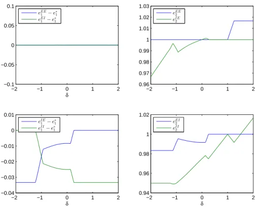
2.1 Welfare difference under bundling and unbundling (v1 = 0.5 andv2 = 0.5). 68 2.2 Optimal effort under bundling (v1 = 0.5 and v2 = 0.5). . . 69
2.3 Optimal effort under bundling (v1 = 0.3 and v2 = 0.7). . . 71
2.4 Optimal effort under bundling (v1 = 0.7 and v2 = 0.3). . . 71
2.5 Dominance regions. . . 72
List of Tables
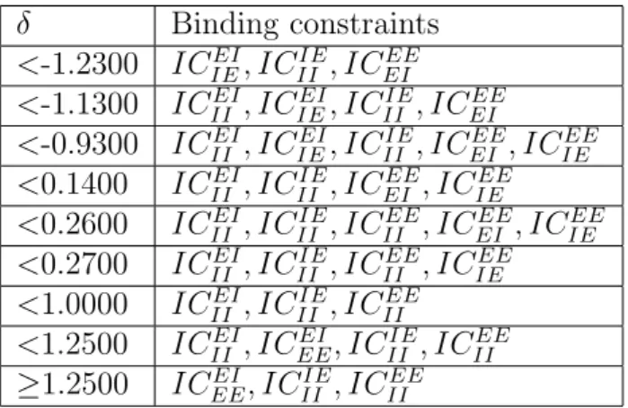
2.1 Binding IC constraints (v1 = 0.5 and v2 = 0.5). . . 70
3.1 Results for benchmark equilibrium - selected values of k . . . 97
3.2 Comparative statics for intertemporal discount rate . . . 98
3.3 Comparative statics for difference of types - 1 . . . 99
3.4 Comparative statics for difference of types - 2 . . . 99
3.5 Comparative statics for lambda - 1 . . . 109
3.6 Comparative statics for lambda - 2 . . . 109
3.7 Comparative statics for v1 - 1 . . . 109
Chapter 1
Simple Contracts under
Simultaneous Adverse Selection and
Moral Hazard
Abstract
We study a principal-agent model with simultaneous moral hazard and adverse selection. In the canonical Grossman and Hart (1983) two-outcome model, we consider the case when agents are risk-neutral and have private information about the outcome distribution conditional on effort. We find that for the simplest case where agents have private information about the outcome distribution only in the case of low effort there may exist no solution. Allowing for a finite number of outcome distributions in case of high effort, we show that the optimal mechanism is characterized by a finite number of contracts, and that the existence problem disappears by increasing the number of types.
1.1
Introduction
Agency problems are usually characterized by the presence of both moral hazard and ad-verse selection elements. Insurance firms, for example, are usually faced with the problem of offering contracts to individuals that are better informed about their riskiness, and which may influence this risk by exerting preventive effort. In such situations, named by Myerson (1982) asgeneralized principal-agent problems, the principal has the joint objec-tive of extracting information from the agents while trying to induce the optimal level of the unobservable action.
one of the them even in situation where both are explicitly present. Notable examples of such cases in the adverse selection literature are the insurance market models of Rothschild and Stiglitz (1976) and Stiglitz (1977), which consider the individual risk as exogenous, and the optimal regulation model of Laffont and Tirole (1986), where the moral hazard dimension is controlled by observability assumptions.
In this paper we study a case where both informational asymmetries arise simultane-ously, under the simplifying assumption that both principal and agent are risk neutral. In a standard moral hazard setting, we explore the case where there are two possible out-comes, stochastically affected by the agents unobservable action. Agents choose between two levels of costly effort, and have private information about the outcome distribution given their choice of effort, as in Gottlieb and Moreira (2013). Types are, therefore, one or two-dimensional vectors, depending on under which level of effort the agents have informational advantage.
In this setting, the efficient allocation is optimal if only one of the agency problems is present. If types are observable, the problem reduces to a pure moral hazard problem. Since both parties are risk-neutral, the principal can implement the first-best by making the agent the residual claimant. If the effort level is observable, the principal can im-plement the first-best by compensating agents for their cost of effort. Since in this case agents would be indifferent, there would be no incentive to deviate.
In the simultaneous presence of both problems, however, the principal needs to leave positive rents for some types in order to induce high effort. The pure moral hazard solution of selling the firm at different values would no longer be feasible, since agents would always deviate and pretend to have a slightly less favourable distribution. By its turn, the adverse selection fixed payments would not implement effort: agents would always choose the higher payment and deviate from the effort recommendation.
We begin our analysis by studying the one-dimensional problems. When agents have private information on the output distribution given high effort, we find that it is optimal for the principal to offer only one contract for all types, characterized by a fixed payment in case of the low outcome, and a positive bonus in case of success. If, however, agents have private information on the output distribution given low effort, no optimal mechanism exists: the principal can arbitrarily approximate the first-best by offering a powerful enough contract.
the success probability given high effort, so there is only a finite number of types in this dimension. While in the continuous case it is not generally possible to fully characterize the solution, our framework allows for more particular results.
We find that our framework leads to a finite number of contracts, limited by the number of possible distributions given high effort. While in the unidimensional case it is not possible to implement effort, and thus there may be no optimal mechanism, we find that this problem becomes less likely when the number of high effort types increases, or when there are types with high enough probability of success given high effort.
Even with our simplicity results, the numerical implementation is not so easy, since the underlying maximization problem is discontinuous. With the use of conditional constrains, however, the problem becomes tractable, although the dimensionality of the problem may pose time and performance constraints for larger number of high effort types.
1.1.1
Related Literature
This paper relates several different lines of work inside the mechanism design literature. The first and most obvious relation is to the heterogeneous literature of mixed models of moral hazard and adverse selection. The results in this literature are highly model-dependent. Since there are many ways for which the problems may interact, the added effects may exacerbate the welfare losses due to informational asymmetry, as in our case, but may as well generate welfare gains when they act in opposite directions.
Laffont and Martimort (2009) provide a simple framework to analyse the effects of the added informational paradigms when the problems do not occur simultaneously. They find that the effect of the added costs to allocative efficiency depends on the timing of the model: for models where the adverse selection occurs before moral hazard (as in our model), adding the costs of the different paradigms may decrease efficiency. For example, the moral hazard dimension may exacerbate the conflict between participation and the adverse selection incentive constraints. On the other hand, in the opposite case where moral hazard occurs before adverse selection, allocative efficiency may be improved.
preventive effort, agents tend to become riskier the higher their coverage. When both problems are simultaneously present, Stewart (1994) argues that they may partially offset each other: since low risk types are offered incomplete coverage because of the adverse selection dimension, they might exert higher effort than under the pure moral hazard contract.
As Stewart (1994), Chassagnon and Chiappori (1997) add preventive effort in Roth-schild and Stiglitz (1976)’s model of competitive insurance markets, characterizing the set of separable equilibria. In a different approach, de Meza and Webb (2001) and Jullien, Salanie, and Salanie (2007) study the case where agents have private information about their risk aversion and may engage in preventive effort. In accordance with the empirical findings of Chiappori and Salanie (2000), who were unable to find a positive correlation between coverage and the probability of accidents in the automobile insurance market, they show that the correlation between risk and coverage is ambiguous and may be even negative.
Another important class of mixed models are the “false moral hazard” models, which can usually be treated as pure adverse selection. In these models, the link between effort, the private information variables and output is deterministic, so agents have no real choice after the output is chosen. Examples are the classic regulation model of Laffont and Tirole (1986) and the seminal taxation model of Mirrlees (1971).
The second relation is to the multidimensional screening literature. By adding private information to the conditional distribution of the outcome in a model where agents can exert two levels of effort, our model features a bi-dimensional screening problem in addition to moral hazard. This kind of model has the added challenge that in general it is not possible to determine the direction in which incentive constraints bind. While usually full characterization is not possible1, some results are known. In the non-linear pricing
framework with a continuum of types, Armstrong (1996) established that it is usually optimal to exclude a positive mass of buyers with low valuations in order to extract more revenue from high valuation ones.
Rochet and Chon´e (1998), in a more general setting, showed that bunching of types is always found in this kind of models, and also that the usual no distortion at the top property of the unidimensional adverse selection models is generalized to the multidi-mensional case (no distortion at the boundary). Finally, Armstrong (1999) showed that multidimensional adverse selection may introduce a simplification of the optimal contract when the private information dimension is high enough.
Our non-existence problem is known in the moral hazard literature. As pointed out by Mirrlees (1999), when the performance signals are arbitrarily informative the first-best may be closely approximated, by means of a contract with sufficiently high penalty in case of an outlying signal. However, since in his example the penalty can always be increased, no limit contract exists. In order to avoid this problem, H¨olmstrom (1979) and Page (1987) introduce upper and lower bounds on payments, in addition to other restrictions on the set of feasible contracts.2 In our case, since there are only two possible outcomes,
lower bounds on payment suffice to avoid this problem.
This lower bound constraint leads to a limited liability problem. In pure moral hazard models with unbounded payments the risk neutrality assumption eliminates any insur-ance problem, so the principal can implement any desired effort level by making the agent the residual claimant, thus rendering the moral hazard problem irrelevant. When limited liability is present, however, the first-best contract may not be feasible, so the principal faces a trade-off between incentives and rent-extraction. This problem, under risk neu-trality, was studied by Innes (1990) in a financial contracting problem, and more recently by Poblete and Spulber (2012) in a more general setting.
Finally, our model relates more closely to the more specific literature on moral haz-ard and adverse selection under risk neutrality. Started by the optimal regulation model of Laffont and Tirole (1986), this literature was further developed by Caillaud, Gues-nerie, and Rey (1992), Melumad and Reichelstein (1989), Picard (1987) and McAfee and McMillan (1987), among others. In this strand of literature, the agent’s choice of effort is not directly observed, but a noisy signal. Since risk-neutrality eliminates the insurance dimension of the problem, Caillaud, Guesnerie, and Rey (1992) argue that this kind of problem can be described as “noisy adverse selection”.
A general result for these models, summarized by Guesnerie, Picard, and Rey (1989), is that the addition of moral hazard does not entail additional welfare loss to the case where actions are observable, even when the distribution of noise is unknown to the principal (but unbiased). In relation to our model, the different results arise from the fact that their analysis focus in the case where the agent’s private information is correlated with their cost, but not the with the noise distribution, while we focus on the opposite case.
This paper is organized as follows. In Section 1.2 we present our framework and a preliminary analysis of the unidimensional cases. Section 1.3 describes our
discrete-2H¨olmstrom (1979) introduces a bounded variation restriction on the feasible contracts. Page (1987)
continuous approach and general results for this setting. In Section 1.4 we analyse the two-type case, while Section 1.5 presents our numerical strategy and some other results.
1.2
The Model
1.2.1
General Setting
We consider the case of a risk-neutral principal and a risk neutral agent in a standard moral hazard setting. The principal is interested in the observable outcomex∈ {xL, xH}, where ∆x=xH−xL >0. This outcome is stochastically influenced by the agent’s actions, which are unobservable. Particularly, we suppose that the agent has the choice of exerting one of two levels of efforte∈ {0,1}.
The agent’s effort has cost ce, such that ∆c= c1 −c0 >0, and agents differ by their
probabilities of success (the occurrence of the outcome x = xH) given effort, which are private information. Their type is denoted by p=(p0, p1), where p0 is the agent’s success
probability givene= 0 and p1 is the probability given e= 1.
The principal has a continuous prior distributionfwith full support on the agent’s type space. Types satisfy the Monotone Likelihood Ratio Property (MLRP), which implies that effort increases the probability of the high outcome, sop1 ≥p0. The type space is defined
by S = {(p0, p1) : p0 ∈ S0, p1 ∈ S1, p1 ≥ p0}. An example of this set is the continuous
case of Gottlieb and Moreira (2013), depicted in the shaded area of Figure 1.1, where
S1 =S0 = [0,1].
p1
p0
1
1
By the Revelation Principle (Myerson, 1981), there is no loss of generality in focusing in direct mechanisms. In this setting, a mechanism is a triple (w, b, e) : S →R2 ×{0,1}, wherew(p) is the payment in the case of low outcome,b(p) is the bonus in case of success ande(p) is the effort recommendation for type p. Given a mechanism (w, b, e) agent type
p expected utility can be written as:
U(p) = w(p) +pe(p)b(p)−ce(p). (U)
For a direct mechanism to be implementable by the principal, it should be optimal for the agent to truthfully announce her type and be obedient to the effort recommendation. For that to happen, a mechanism should satisfy the incentive-compatibility constraints:
U(p)≥w(ˆp) +peˆb(ˆp)−cˆe,∀p,pˆ,e.ˆ (IC) Additionally, it should be optimal for the agent to participate in the mechanism. For that to happen, her expected payoff should be higher than her reserve utility, which we consider as type-independent and normalize to zero. The individual rationality constraints can then be written as:
U(p)≥0,∀p. (IR)
We also assume free disposal, so the agent can reduce the output without cost. This restriction implies that payments have to be increasing in the level of output:
b(p)≥0,∀p. (FD)
We say that a mechanism that satisfies (IC), (IR) and (FD) is feasible. Given a mechanism (w, b, e), the principal’s expected payoff is:
ˆ
S
[xL−w(p) +pe(p)(∆x−b(p))]f(p)dp. (W)
We say that a mechanism is optimal if it maximizes the principal’s payoff over the set of feasible mechanisms. Two feasible mechanisms areequivalent if all agent types are indifferent between them and both give the same level of utility to the principal.
and therefore
eF I(p) =
1 if p0 < p1− ∆∆xc
0 otherwise. (1.1)
In the remainder of this section we will present a simple preliminary analysis of the uni-dimensional cases, before extending to more general settings. In the analysis that follows, we restrict ourselves to the main results for each case, leaving the detailed for presentation the next section.
1.2.2
Unidimensional Analysis
Adverse Selection in p1
In this case, agents have private knowledge of the outcome distribution conditional on high effort only. Since the outcome distribution conditional on low effort is constant and known, p = (¯p0, p1) for known ¯p0. For example, a manager may decide to leave the
company unattended, in which situation the outcome has a known distribution, but she may have more knowledge about the profitability of her actions in case of effort.
Since the outcome conditional on low effort does not depend on the agent’s type, all agents for which the principal recommends low effort should have the same expected payoff in a feasible mechanism. To induce effort, the principal must pay a positive bonus, which, as the expected outcome, should be non-decreasing on the agent’s type.
In such situation, any feasible mechanism should have that if high effort is recom-mended for some typep= (¯p0, p1), then it is also recommended for all types with higher
success probability. To see this, consider a mechanism such that e(p) = 1 and e(ˆp) = 0 for some type ˆp = (¯p0,pˆ1) such that ˆp1 > p1. Since, to induce effort, the principal must
pay a positive bonus to type p, incentive compatibility dictates that U(ˆp) > U(p). On the other hand,p can mimic ˆp without cost, so we must have U(p)≥U(ˆp).
The above conditions, together with the individual rationality and the free disposal constraints, imply that an optimal contract should give zero expected utility to all agents who do not exert effort. Since both the bonus and expected utility should be increasing on the agent’s type for those who exert effort, but are costly to the principal, in the optimal mechanism the principal offers a single contract to all agents.
Proposition 1. If agents have private information on p1 only, then any optimal
(non-trivial) mechanism is equivalent to a mechanism characterized by an effort threshold ξ such that e(p) = 1 if and only if p1 > ξ, and a single contract (w, b) = ( ¯w,¯b) such that
U(¯p0,p¯0) = 0 and ¯b = ξ−∆pc¯0, which is the minimal bonus that induces effort.
Adverse Selection in p0
In this case, the outcome distribution conditional on high effort is known, but the distri-bution conditional on low effort is private information. This may be the case for some insurance scenarios, where effort may be the adoption of a security device or procedure for which the risk is known.
As before, to induce high effort the principal must pay a positive bonus, but since all agents have the same expected outcome given high effort, their expected payoff has to be constant. Differently from the previous case, to induce effort the principal may need to leave positive rents to agents who exert low effort.
In special, this setting introduces the possibility of an agent type who can mimic any other type effortlessly. The expected outcome of typep= (¯p1,p¯1) is constant, so it never
exerts high effort. Since it has the same success probability than any type that does exerts high effort, it has to receive the same expected payment as these types, without having to incur in the additional cost. Consequently, any close enough type should receive positive rents too.
Parallel to the previous case, we can restrict ourselves to mechanisms such that the effort recommendation can be represented by an effort thresholdξsuch that e(p0,p¯1) = 1
if and only ifp0 < ξ. The intuition for this result is as follows. If the principal recommends
low effort for type p = (p0,p¯1), then any agent ˆp = (ˆp0,p¯1) with ˆp0 > p0 has even less
incentive to exert effort. If type ˆp is indifferent between exerting high or low effort, then the principal can improve by asking him to exert low effort.
As mentioned above, in the region of high effort all agents must receive the same contract. In the region of low effort, incentive compatibility implies that the agent’s expected utility and bonus should be increasing in their type. Additionally, the global incentive constraint implies that type p = (¯p1,p¯1) should receive the same expected
payment as those types who exert high effort, plus the cost differential.
equal to ∆c. In particular, the principal’s problem is that of finding an increasing convex functionU such that U(ξ) = 0 and U(¯p1) = ∆c.
This leads to the main result of this section:
Proposition 2. If agents have private information onp0 then the principal can arbitrarily
approximate the first-best solution. There exists no optimal mechanism that implements effort.
To see the intuition for this result, suppose the principal wants to implement an effort threshold ξ > 0. Since leaving informational rent is costly, she will want to leave zero rent for as many types as possible. In particular, it is feasible to offer a trivial contract to all types until p1 −ǫ, and a single high-powered contract for all types above so that
U(p1) = ∆c. By decreasing ǫand offering an even higher powered contract, the principal
decreases the expected payment. Since the bonus is unbounded, and it is not feasible to offer infinite bonus, there is no optimal mechanism that implements the effort threshold
ξ.
1.3
The Discrete-Continuous Approach
This section extends the analysis of the previous section to more general type spaces. In order to better study the main characteristics of the unidimensional setting and that of Gottlieb and Moreira (2013), specially the introduction of the global incentive compatibil-ity constraints, we let p1 assume only a finite number n of values, soS1 ={p11, p21, ..., pn1}.
This type space is represented by the horizontal lines in Figure 1.2.
p1
p0
p1 1
p2 1
p3 1
1.3.1
Optimal Mechanisms
In this subsection we describe the conditions for the optimality of a mechanism. Our first lemma is a direct consequence of the effort conditions proved in Propositions 1 and 2:
Lemma 1. For any optimal mechanism, there exists an equivalent mechanism (w,b,e)
such thate(p0, p1) = 1if and only ifp0 < ξ(p1)for a non-decreasing functionξ:S1 →[0,1]
Lemma 1 states that we can restrict ourselves to the case where the effort function
e(p) can be represented by an increasing function in the set S1, the boundary between
the low and high effort intervals given a probability of success given high effort p1. We
refer to this function ξ as the effort frontier of a mechanism.
The intuition for this result is simple, and follows directly from the discussion in Section 2. If agent type p = (p0, p1) exerts low effort, then any type ˆp = (ˆp0, p1), with
ˆ
p0 > p0 has a higher incentive to exert low effort. Similarly, if agent type p = (p0, p1)
exerts high effort, then any type ˆp = (p0,pˆ1), with ˆp1 > p1 has higher incentive to exert
high effort.
By restricting our analysis to mechanisms such that the effort recommendation func-tion can be represented by an increasing funcfunc-tion ξ :S1 →[0,1], incentive compatibility
implies the following necessary conditions for optimality3:
Lemma 2 (Necessary Conditions). If a mechanism is optimal, there exists an equivalent mechanism(w, b, e), with associated effort frontier and informational rent functionsξ and U, such that:
a. U(p0, p1) is convex in p0 and has derivative equal to b(p0, p1) if p0 > ξ(p1) and zero
otherwise.
b. ∆p1U(p0, p1) ≥ b(p0, p1)∆p1 and ∆p1b(p0, p1) ≥ 0 if p0 < ξ(p1), while U(p0, p1) is constant in p1 otherwise;
c. b(p0, p1) is constant in p1 for p0 > ξ(p1) and constant in p0 if p0 < ξ(p1);
d. U(0, p1)≥0 and b(0, p1)≥0;
e. if p0 < ξ(p1), U(p0, p1) = U(p1, p1)−∆c;
f. b(p1, p1) =b(p0, p1) for almost all (p0, p1) such that p0 < ξ(p1);
3
In what follows, we use the convention that ∆p1f(·, pi1) =f(·, pi +1
1 )−f(·, p
i
Conditions (a)-(c) follow directly from the first and second order condition for incen-tive compatibility, which requires truthfully reporting by each type while following the principal’s effort recommendation. These three conditions, controlled by the effort level, are the usual local conditions for incentive compatibility in pure adverse selection models.
Condition (d) follows directly from the individual rationality and free disposal, and conditions (e) and (f) are the global incentive compatibility constraints, briefly described in the previous section. Since effort is costly, there is no feasible mechanism that implements effort for the diagonal types (p1, p1). Because those types can mimic any other type on
the same line without cost, incentive compatibility dictates that they must get the same expected payment as those bellow the effort frontier.
While it is known that in models of pure adverse selection conditions (a)-(d) are also sufficient for feasibility, in our model the moral hazard dimension introduces a new set of necessary conditions. Lemma 3 establishes that these necessary conditions are also sufficient.
Lemma 3. Let (w, b, e) be a mechanism satisfying the condition that e(p0, p1) = 1 if and
only if p0 < ξ(p1) for a non-decreasing function ξ : S1 → [0,1]. Suppose that conditions
(a)-(f) are satisfied. Then,(w, b, e) is a feasible mechanism.
Lemmata 2 and 3 establish that for any optimal mechanism there is an equivalent mechanism that satisfies conditions (a)-(f). By Lemma 3, any mechanism satisfying these conditions is feasible. For notational simplicity, henceforth we will denote by (w, b, ξ) this equivalent mechanism. Thus we have established the following characterization result:
Proposition 3. A mechanism is optimal if and only if there exists an equivalent mecha-nism(w, b, ξ) that satisfies (a)-(f) and such that(w, b, ξ)maximizes the principal’s payoff.
1.3.2
One-Dimensional Projection
The usefulness of the characterization of Proposition 3 is limited by the fact that its associated program is not very tractable as stated. In this section, we will show that we can write it as an unidimensional program.
Gottlieb and Moreira (2013) show that, in the continuous type case, both the informa-tional rent function and the effort frontier can be recovered from informainforma-tional rent left to the types in the diagonal line (p1, p1). Therefore the problem of finding a feasible
Since we only have a finite number of such elements, it is not possible to recover the informational rent of all types by those in the diagonal. Nevertheless, by using a similar strategy, we prove that there exists a unidimensional function with this property.
The following lemma proves the existence of such function, and how it is constructed:
Lemma 4. Let (w, b, ξ) be an optimal mechanism and let ξF I denote the efficient,
full-information, effort frontier. There exists a continuous, non-negative, increasing convex function U such that U(0) = 0 and
U(p0, p1) =
U(p0) if p0 > ξ(p1)
U(p1)−∆c otherwise
(1.2)
b(p0, p1) =
˙
U(p0) if p0 > ξ(p1)
˙
U(p1) otherwise
(1.3)
w(p0, p1) =
U(p0)−p0U˙(p0) if p0 > ξ(p1)
U(p1)−p1U˙(p1) otherwise
(1.4)
ξ(p1) =
U−1(U(p
1)−∆c) if U(p1)>∆c
min{max{U−1(0)}, ξF I(p
1)} if U(p1) = ∆c
0 otherwise
(1.5)
Lemma 4 states that any optimal non-trivial mechanism can be characterized by a continuously increasing functionU, which we will call arent projection of the mechanism. By (1.2) it can be seen that this function represents the informational rent left to the agents that exert low effort, while it recovers the rent left to those who exert effort by the global incentive compatibility condition (e) of the diagonal types.
It is important to note that, in order to represent a feasible mechanism (w, b, ξ), U
need only to be defined forp0 if there is any p1 ∈S1 such that low effort is recommended
for type (p0, p1). A priori, this function could assume any value for p0 if p0 < ξ(p1) for
all p1; in particular, we only prove that there exists a continuous function U such that
U(p0)=U(p0, p1) whenp0 > ξ(p1) for somep1 ∈S1, without further restrictions other than
The recovery of the bonus function (1.3) for those types who exert low effort follows directly from the local incentive compatibility conditions (a) and (c), while the bonus for those who exert high effort, which is constant inp0 by (c), follows from the moral hazard
condition (f). The recovery of the fixed paymentw follows from the definition ofU.
While in the continuous case the effort frontier associated to a payment scheme is unique for any feasible mechanism, in our case the same does not hold. If U equals zero for an interval, and U(p1) = ∆cfor some p1, then any type in the interval would be
indifferent between exerting high or low effort. However, since no rent would be needed to induce effort in this interval, in such cases the principal would be better off by increasing the effort region until its full information level. Therefore, by (1.5), optimality implies that the effort frontier can be uniquely recovered from the rent projection.
Conversely to the construction of the rent projection, Corollary 1 shows that the problem of finding the optimal mechanism can be reduced to the problem of finding an optimal rent projection.
Corollary 1. For any continuous, increasing, non-negative convex function U there is a feasible mechanism (w, b, ξ) such that U is one of its rent projections.
Given Corollary 1, the principal’s problem is reduced to
W∗ = max
U,ξ
X
S1
ˆ ξ(pi1)
0
[pi
1∆x− U pi1
]f(p0, pi1)dt
+X S1
ˆ pi1
ξ(pi 1)
[p0∆x− U(p0)]f(p0, pi1)dt
(P)
subject to U non-negative, continuously increasing and convex, and the effort condition (1.5).
1.3.3
Finite Contracts
The following definition of continuous piecewise linear functions, partially borrowed from Aliprantis, Harris, and Tourky (2006), will be useful for our future analysis:
Definition 1(Piecewise linear function). A function f : [t, t]→R, where [t, t] is a closed interval of R, is a piecewise linear function if there exists a partition t = t1 < t2 <
... < tk =t and real constants x0, b1, ..., bk such that for each x∈[t, t]
f(x) =x0+
k
X
i=1
bi(x−ti)+.
Forb0 = 0, we say thatti is a breakpoint of f if i < k and bi 6=bi−1.
We are thus ready for our main characterization result:
Proposition 4. The optimal rent projection function U∗ is a piecewise linear function with at most 2n−1 breakpoints such that:
a. U∗ has a constant slope in [pn−1 1 , pn1].
b. if ξ∗ < ξF I, then U∗ has at most one breakpoint inside each of the intervals
[0, p1
1], ...,[pn1−2, pn1−1];
Proposition 4 tells us that we can focus on mechanisms such that the principal offers only a finite number of contracts, a strong simplicity result. Furthermore, the linearity result implies that the rent projection associated with an optimal mechanism is unique. Additionally, it gives us conditions on the regions where the bonus may change when the effort frontier is below its efficient level, while implying that the bonus should be constant in the last interval, [pn−1
1 , pn1].
The rationale for this result can be seen in Figure 1.3. For any convex function, we can construct another feasible extended rent projection by taking the maximum of the lines tangent to the function at the points p1. This mechanism would be able to implement a
higher effort frontier ˆξ at a smaller cost to the principal.
U(p)
p p2
1
p1
1 ξ(p21)
ξ(p1 1)
(a) Feasible rent projection and associated effort frontierξ
U(p)
p p2
1
p1
1 ξ(p21)
ξ(p1
1) ξˆ(p11)
ˆ
ξ(p2 1)→
(b) Alternative rent projection and effort frontier ˆξ
Figure 1.3: Linearity of the Optimal Mechanism
it is possible to implement the same effort frontier at a lower cost. Since the principal can always lower the expected payment by offering a higher-powered contract for a smaller interval of types at the top, in any optimal mechanism the bonus should be constant in the interval [p1
1, p21].
Proposition 5. Let W∗ be the supremum value of problem (P). Allowing for disconti-nuities at the top, there exists a positive, convex, increasing function U∗∗, and an effort frontier ξ∗∗ that together satisfy the effort condition (1.5) and that W(U∗∗, ξ∗∗) =W∗.
Although Proposition 5 does not provide a feasible mechanism, it provides a simple way to write the problem such that a solution is guaranteed. In the next section this proposition is used to characterize the existence in the simple setting whereS1 has only
two elements.
Before moving to more specific settings, we further develop some characteristics of an optimal mechanism, which follow directly from the arguments of Proposition 4:
Lemma 5. Let (w, b, ξ) be an optimal non-trivial mechanism, and let p∗
1 = min{p1 ∈
S1 : ξ(p1) > 0} and U be, respectively, the first type p1 to exert high effort and the rent
projection associated with it. Then:
a. U(ξ(p∗
1)) = 0 and U(p∗1) = ∆c;
b. U has one and only one breakpoint in the interval [ξ(p∗
1), p∗1).
Lemma 5 provides a further simplification on the set of optimal mechanisms. Since leaving rents is costly and it is only needed in order to implement effort, any optimal mechanism will leave zero rent for p0 ≤ ξ(p∗1). Consequently, by the previous linearity
arguments, there should be only one breakpoint belowp∗
1.
1.4
The Two-Type Case
In this section, we work with the case in whichS1 ={p11, p21}. Our first result follows from
the arguments in Proposition 1 and Lemma 5.
Lemma 6. There is no optimal mechanism such that ξ(p1
1) = 0 and ξ(p21)>0.
Lemma 6 implies that any optimal mechanism should implement effort for all typesp1,
or the trivial contract. The reason for this result follows the one-dimensional reasoning: any effort frontier such that ξ(p1
1) = 0 and ξ(p21) > 0 can be implemented by offering a
This existence result implies that there are only two possible kind of solutions for the principal’s problem, a trivial mechanism that implements low effort only, and a mechanism with only one positive-bonus contract such that ξ(p1
1) >0, implementing high effort for
both types.
By Proposition 5 we know the supremum of the principal’s problem can be achieved by relaxing the continuity restriction at the top. For n = 2, this relaxed problem can be written as
max
0≤t1≤p11
0≤ξ(p1 1)≤t1
ǫ>0
W =
ˆ ξ(p11)
0
[p11∆x−∆c]f(p0, p11)dp0+ ∆x
ˆ t1
ξ(p1 1)
p0f(p0, p11)dp0
+
ˆ p11
t1
[p0∆x−b(p0−t1)]f(p0, p11)dp0+
ˆ ξ(p21)+ǫ
0
[p21∆x−b(p21−t1+ǫ)]f(p0, p21)dp0
+
ˆ p21
ξ(p2 1)
[p0∆x−b(p0−t1)]f(p0, p21)dp0
where
b=
0 if t1 = 0 ∆c
p1
1−t1 otherwise
ξ(p21) =
0 if t1 = 0
p2
1−p11+t1 otherwise
The main difference from this problem to the original one, given by (P), is the inclusion of the variable ǫ, which represents the discontinuity and allows an increase in the effort region from the original contract, given by the breakpointt1 and its corresponding bonus
b. This increase comes together with an additional expected payment b×ǫfor all (p0, p21)
in the high effort region, in order to satisfy the global incentive constraints.
In what follows, we present an exploration of the different solutions for this case. For simplicity, we suppose that the conditional distribution of p0 given p1 is uniform in the
Solution 1: Trivial contract
In the trivial case, we have that t1, ξ(p11) and ǫ are all equal to zero. Consequently, the
principal’s welfare can written as
W1 = ∆x
ˆ p11
0
p0f(p0, p11)dp0 + ∆x
ˆ p21
0
p0f(p0, p21)dp0
= ∆xP1p
1
1 +P2p21
2 .
This trivial contract solution is optimal only when ξF I
2 = 0:
∆x
∆c <
1
p2 1
=η1.
Solution 2: Trivial contract with effort for the high type
In this case, t1 and ξ(p11) are equal to zero, but ǫ is positive. Therefore, ǫ assumes the
first best value of ξ(p2
1), and welfare amounts to
W2 = ∆x
ˆ p11
0
p0f(p0, p11)dp0+
ˆ ξF I(p21)
0
[p21∆x−∆c]f(p0, p21)dp0 + ∆x
ˆ p21
ξF I(p2 1)
p0f(p0, p21)dp0
= 1 2P1p
1
1∆x+P2(−2∆c+
∆c2
∆xp2 1
+ 2∆xp21) =W1+P2
(∆c−p2 1∆x)2
2p2 1∆x
This solution is not feasible in the original restricted problem. It happens if and only if
η1 ≤
∆x
∆c ≤η2,
for some η2 > p11
1. While it is clear that it happens when ξ
F I(p1
1) = 0 and ξF I(p21)>0, in
which case it achieves the first-best, it also happens when ξF I(p1
1) is positive and small,
Solutions 3 and 4: Only one contract with positive power
In this case there is only one contract with positive power, so both t1 and ξ(p11) are
positive, whileǫ equals zero. In this case
W3 =
ˆ ξ(p11)
0
[p11∆x−∆c]f(p0, p11)dp0+ ∆x
ˆ t1
ξ(p1 1)
p0f(p0, p11)dp0
+
ˆ p11
t1
[p0∆x−b(p0 −t1)]f(p0, p11)dp0 +
ˆ ξ(p21)
0
[p21∆x−b(p21−t1)]f(p0, p21)dp0
+
ˆ p21
ξ(p2 1)
[p0∆x−b(p0 −t1)]f(p0, p21)dp0
Two solutions are possible. Since the payoff for p0 < t1 equals zero, the principal
can always lower the effort frontier at no cost by offering a contract with zero bonus in addition to the powered contract. For that reason, it may be optimal for the principal to choose an effort frontier different than the breakpointt1.
In the solution 3, we have thatt1 =ξ(p11). For this case, we have that, by the first-order
condition and concavity of the problem,t1 is the solution to
∆x(p1
1−t1)− ∆c2
P1
p1
1 + n
∆x(p1
1−t1)−∆c
h
1
2 +
(p2 1−p
1 1)
(p1 1−t1) +
(p2 1−p
1 1)(p
2 1−p
1 1+t1)
(p1 1−t1)2
io
P2
p2
1 = 0. (1.6)
Given t1, it is only optimal to increase ξ(p11) until its first-best value. That way, in
a solution of this kind, t1 = ξ(p11) ≤ ξF I(p11). Conversely, if t1 6= ξ(p11), then ξ(p11) =
ξF I(p1
1)< t1,where t1 is the solution to
∆x(p1
1−t1) + ∆c2
P1
p1
1 + n
∆x(p1
1−t1)−∆c
h
1
2 +
(p2 1−p11)
(p1 1−t1) +
(p2
1−p11)(p21−p11+t1)
(p1 1−t1)2
io
P2
p2
1 = 0.
Solution 5: Positive power and extra effort for the high type
In this case, the principal wishes to add more effort on the second interval, when the effort frontier is already positive. We have then thatt1, ξ(p11) and ǫ are positive. Of course, as
The payoff of the principal is
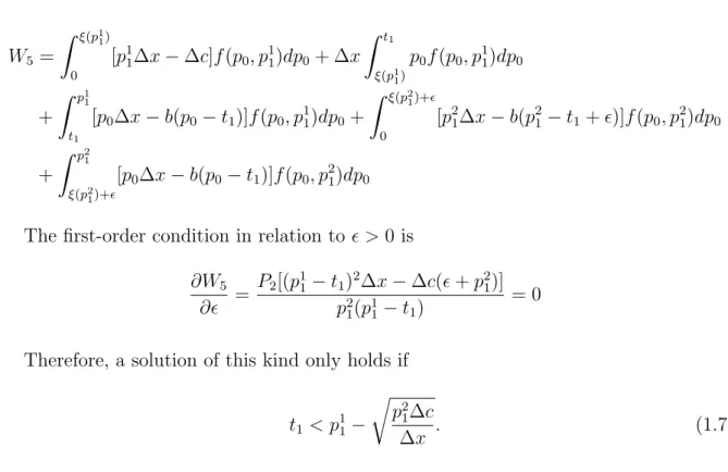
W5 =
ˆ ξ(p11)
0
[p11∆x−∆c]f(p0, p11)dp0+ ∆x
ˆ t1
ξ(p1 1)
p0f(p0, p11)dp0
+
ˆ p11
t1
[p0∆x−b(p0−t1)]f(p0, p11)dp0+
ˆ ξ(p21)+ǫ
0
[p21∆x−b(p21−t1+ǫ)]f(p0, p21)dp0
+
ˆ p21
ξ(p2 1)+ǫ
[p0∆x−b(p0−t1)]f(p0, p21)dp0
The first-order condition in relation toǫ >0 is
∂W5
∂ǫ =
P2[(p11−t1)2∆x−∆c(ǫ+p21)]
p2
1(p11−t1)
= 0
Therefore, a solution of this kind only holds if
t1 < p11−
r p2
1∆c
∆x . (1.7)
The result from our analysis of the different solutions for this case is summarized in the following proposition:
Proposition 6. There exist η1, η2 andη3 such that an optimal mechanism exists if ∆∆xc ∈
[0, η1]∪[η2, η3], and lim
p1 1→p
2 1
η2−η1 = 0 and lim
p1 1→p
2 1
η3 =∞.
This claim can be seen in Figures 1.4 and 1.5. It is quite clear that the optimal mechanism exists in two disjoint intervals. Initially, the optimal mechanism is trivial, and after a non-existence region where the first-best can be arbitrarily approximated, the optimal mechanism is given by a single contract with positive bonus. When the benefit from effort (i.e, the success outcome) is very large, however, it becomes interesting for the principal to pay for more effort from those types on the top. In this case, no optimal mechanism exists.
Figure 1.5 shows our second claim. When types are very close, the existence intervals increase. In fact, while in the case where p1
1 = 0.5 no optimal mechanism exists for
∆x >30, when p1
0 5 10 15 20 25 30 35 40 45 50 0 0.05 0.1 0.15 0.2 0.25 0.3 0.35 ∆x t1 t1
ξ(p1 1)
0 5 10 15 20 25 30 35 40 45 50
0 0.1 0.2 0.3 0.4 0.5 0.6 0.7 0.8 0.9 1 ∆x ǫ
Figure 1.4: Two-Type Case - p1
1 =.5, p21 = 1.
0 10 20 30 40 50 60 70 80 90 100
0 0.1 0.2 0.3 0.4 0.5 0.6 0.7 0.8 0.9 ∆x t1 t1
ξ(p1 1)
0 10 20 30 40 50 60 70 80 90 100
0 0.1 0.2 0.3 0.4 0.5 0.6 0.7 ∆x ǫ
Figure 1.5: Two-Type Case - p1
1 =.9, p21 = 1.
1.5
The n-Type Case
In this section we explore numerical strategies for the general n-type case. In particular, we present some alternative approaches and our results for some preliminary examples. As in Section 1.4, we allow for a discontinuity at the top by the use of a variableǫ >0.
1.5.1
Numerical Approach
When a solution exists, the maximization problem (P) restricted to j contracts be-comes
max
0≤t1≤t2≤...≤tj
0≤b1≤b2≤...≤bj
W =
n
X
i=1
ˆ ξ(pi1)
0
[pi
1∆x− U pi1
]f(p0, pi1)dp0
+ n
X
i=1
ˆ pi1
ξ(pi 1)
[p0∆x− U(p0)]f(p0, pi1)dp0
(P1)
s.t.
U(x) = j
X
i=1
bi(x−ti)+.
ξ(p1) =
U−1(U(p
1)−∆c) if U(p1)>∆c
min{max{U−1(0)}, ξF I(p
1)} if U(p1) = ∆c
0 otherwise.
While easily implementable, this formulation suffers from several drawbacks. First, it is discontinuous at any point thatU(p1) = ∆c. Second, it contains several local maxima.
Lastly, it depends on the exogenous variablej, which represents the numbers of contracts with positive bonus.
One way to avoid the discontinuity whenU(p1) = ∆cis to let p∗1 be a choice variable.
Thus, by Lemma 5, U(p∗
1) = ∆c, and there is one and only one breakpoint below p∗1.
Consequently, b1 becomes endogenous through t1. Therefore, it is easier to rewrite the
problem as a function of the incremental bonus zi =bi−bi−1. Conditional on p∗1 and j,
problem P becomes
max
0≤t1≤p∗1
t2≤...≤tj
0≤zi
W =
n
X
i=1
ˆ ξ(pi1)
0
[pi
1∆x− U pi1
]f(p0, pi1)dp0
+ n
X
i=1
ˆ pi1
ξ(pi 1)
[p0∆x− U(p0)]f(p0, pi1)dp0
(P2)
s.t.
U(x) = j
X
i=1
bi = ∆c p∗
1−t1 if i= 1
bi−1+zi otherwise
ξ(p1) =
U(p1)−∆c if U(p1)>∆c
min{t1, ξF I(p1∗)} if U(p1) = ∆c
0 otherwise.
While this formulation avoids the discontinuity problem, it is still subject to multiple local maxima. In particular, any solution for a problem withj contracts is a local optimal in the problem with j+ 1 contracts with tj+1 =tj and cj+1 = 0.
Up until now, we have ignored the fact that in most cases there is at most one break-point in each of the intervals [pi
1, p
i+1
1 ]4. An alternative approach is thus to allow for a
variable number of breakpoints, maximizing on a partition of U. Let i∗ = min{i < n : ξ(pi
1)>0}. Givenp1∗, we search for j =n−i∗ contracts, and the problem can be written
as
max
0≤t1≤p∗1
pi1∗+i−1≤ti≤pi ∗+i 1
0≤zi
W =
n
X
i=1
ˆ ξ(pi1)
0
[pi1∆x− U pi1]f(p0, pi1)dp0
+ n
X
i=1
ˆ pi1
ξ(pi 1)
[p0∆x− U(p0)]f(p0, pi1)dp0
(P3)
s.t.
U(x) = j
X
i=1
bi(z−ti)+.
bi =
∆c p∗
1−t1 if i= 1 bi−1+ci otherwise
ξ(p1) =
U(p1)−∆c if U(p1)>∆c
min{t1, ξF I(p1∗)} if U(p1) = ∆c
0 otherwise.
This approach deals with both the continuity and local minimum problems of previous
4While we conjecture that this is a property of any optimal mechanism, and could not reproduce
formulations. However, it significantly increases the dimension of the problem. Neverthe-less, it has proven to be quite robust when the dimension is low (n <50).
In our exploration, several other approaches were proposed and tested. In particular, we tried to treat the effort frontierξas exogenous, since these variables are bounded by the pointsp1. We have found, however, that the nonlinear constraints necessary to guarantee
feasibility complicate the problem significantly, and performance was poor even when dealing withn= 4 and standard local optimization algorithms for continuous functions.
1.5.2
Numerical Exercises
For our numerical exercises, we worked with equally spaces points p1 ∈ [0,1] distributed
with equal probabilities, so that the probability of p1 was given by P(p1) = 1n and the
conditional probability of p0 given p1 was given by the density function f(p0|p1) = p11.
Additionally, we set ∆c= 1, varying only the number of types p1 and ∆x.
All optimization procedures were implemented in MATLAB5, with the use of the
opti-mization solver KNITRO (Byrd, Nocedal, and Waltz, 2006) for the conditional problems. In particular, we have found more accurate results for the program (P2) by the use of their interior-point algorithm with multiple starting points, while the solution for program (P3) was found significantly faster and accurately with their active-set algorithm.
Program (P2), due to the discussed issues, was found to be highly dependent on the chosen starting point. Nevertheless, the local optimization is fast enough so that it is feasible to use thousands of random starting points if necessary. Program (P3) was found to be robust to the choice of starting points for n < 50, with the dimensionality of the problem starting to pose performance constraints afterwards.
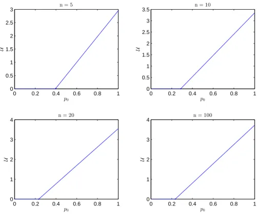
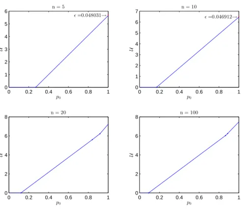
In Figures 1.6, 1.7 and 1.8 we present the result of our simulations for ∆x = 20,30 and 100. It can be seen that the existence problem discussed in the previous sections is still present even for large number of contracts when ∆x is large. It, however becomes less likely when the number of contracts increase.
0 0.2 0.4 0.6 0.8 1 0 0.5 1 1.5 2 2.5 3
n = 5
U
p0
0 0.2 0.4 0.6 0.8 1
0 0.5 1 1.5 2 2.5 3 3.5
n = 10
U
p0
0 0.2 0.4 0.6 0.8 1
0 1 2 3 4
n = 20
U
p0
0 0.2 0.4 0.6 0.8 1
0 1 2 3 4
n = 100
U
p0
Figure 1.6: Numerical simulations: ∆x= 20.
0 0.2 0.4 0.6 0.8 1
0 1 2 3 4 5
ǫ=0.014557→
n = 5
U
p0
0 0.2 0.4 0.6 0.8 1
0 1 2 3 4 5
ǫ=0.0138→ n = 10
U
p0
0 0.2 0.4 0.6 0.8 1
0 0.5 1 1.5 2 2.5 3 3.5
n = 20
U
p0
0 0.2 0.4 0.6 0.8 1
0 0.5 1 1.5 2 2.5 3 3.5
n = 100
U
p0
0 0.2 0.4 0.6 0.8 1 0 1 2 3 4 5 6
ǫ=0.048031→
n = 5
U
p0
0 0.2 0.4 0.6 0.8 1
0 1 2 3 4 5 6 7
ǫ=0.046912→
n = 10
U
p0
0 0.2 0.4 0.6 0.8 1
0 2 4 6 8
n = 20
U
p0
0 0.2 0.4 0.6 0.8 1
0 2 4 6 8
n = 100
U
p0
Figure 1.8: Numerical simulations: ∆x= 100.
The number of contracts also seems to increase with both ∆x and n. While for ∆x = 20 it is optimal to offer only one contract for all types, this number increases to two for ∆x= 30 and three for ∆x= 100. The gains from finer discretizations also seem limited, with no particular informative gains from n= 20 to n= 100.
1.6
Conclusion
In the canonical Grossman and Hart (1983) two-outcome model, we considered the case when agents are risk-neutral and have private information about the outcome distribution conditional on effort. While in most of the literature on simultaneous moral hazard and adverse selection, specially on paper focuses on the phenomenon under risk neutrality, the added informational problems do not generate greater welfare loss than only one of them, in our case the same does not hold: while any of the individual asymmetry problems is irrelevant by itself, together they pose significant constraints on efficiency, and consequently on welfare.
not exist, with the principal being able to arbitrarily approximate the first-best. When their private information is on the distribution given high effort, any optimal mechanism that implements high effort is equivalent to a single contract for all agents. In this case, agents who exert low effort have all their rent extracted, while agents who exert high effort are left with positive rents.
In our bi-dimensional framework, where the distribution of high-effort types is discrete, most of these results still hold. We find that optimal contracts are simple, in that any optimal mechanism is equivalent to the principal offering a number of contracts smaller than the number of high-effort types. Therefore, the problem becomes as that of finding the the parameters that characterize a piecewise linear function. The existence problem still exists, albeit limited to a smaller region where there is no optimal way to induce additional effort.
When studying the case of two high-effort types, we show that there are three possible types of optimal mechanism: one when where the principal offers a trivial contract and all agents exert low effort, and two where the principal offers only one contract with positive bonus, accompanied or not by a contract where the principal only covers the cost of low effort. However, an optimal contract does not exist in two cases, a region where the gain of effort is small and the first best can be approximated, and a region where it is very large and the principal may want to buy additional effort.
Even with our simplicity results, the numerical implementation is not so easy, since the underlying maximization problem is discontinuous. With the use of conditional con-straints, however, the problem becomes tractable, although the dimensionality of the problem may pose time and performance constraints for larger number of high effort types. In spite of any dimensionality problem, we were able to perform simulations with large (as high asn= 100) number of types for both of our proposed numerical programs.
1.7
References
Aliprantis, C. D., D. Harris,andR. Tourky(2006): “Continuous Piecewise Linear Functions,” Macroeconomic Dynamics, 10(01), 77–99.
Armstrong, M.(1996): “Multiproduct Nonlinear Pricing,”Econometrica, 64(1), 51–75.
(1999): “Price Discrimination by a Many-Product Firm,” The Review of Eco-nomic Studies, 66(1), 151–168.
Armstrong, M., and J. Rochet (1999): “Multi-Dimensional Screening: A User’s Guide,” European Economic Review, 43(4-6), 959–979.
Arnott, R. J., and J. E. Stiglitz (1988): “The Basic Analytics of Moral Hazard,”
Scandinavian Journal of Economics, 90(3), 383–413.
Byrd, R. H., J. Nocedal, and R. A. Waltz (2006): “KNITRO: An Integrated Package for Nonlinear Optimization,” inLarge-scale nonlinear optimization, pp. 35–59. Springer.
Caillaud, B., R. Guesnerie, and P. Rey (1992): “Noisy Observation in Adverse Selection Models,” The Review of Economic Studies, 59(3), 595–615.
Chassagnon, A., and P.-A. Chiappori (1997): “Insurance under Moral Hazard and Adverse Selection: The Case of Pure Competition,” DELTA-CREST Working Paper.
Chiappori, P.-A., and B. Salanie (2000): “Testing for Asymmetric Information in Insurance Markets,” Journal of Political Economy, 108(1), 56–78.
de Meza, D.,andD. C. Webb(2001): “Advantageous Selection in Insurance Markets,”
RAND Journal of Economics, 32(2), 249–62.
Gottlieb, D., and H. Moreira (2013): “Simultaneous Adverse Selection and Moral Hazard,” Working Paper.
Grossman, S. J., and O. D. Hart(1983): “An Analysis of the Principal-Agent Prob-lem,” Econometrica, 51(1), 7–46.
Guesnerie, R., P. Picard, andP. Rey(1989): “Adverse Selection and Moral Hazard with Risk Neutral Agents,” European Economic Review, 33(4), 807–823.
Innes, R. D.(1990): “Limited Liability and Incentive Contracting with Ex-Ante Action Choices,” Journal of Economic Theory, 52(1), 45 – 67.
Jullien, B., B. Salanie, and F. Salanie (2007): “Screening Risk-Averse Agents Under Moral Hazard: Single-Crossing and the CARA Case,” Economic Theory, 30(1), 151–169.
Laffont, J., and J. Tirole (1986): “Using Cost Observation to Regulate Firms,”The Journal of Political Economy, 94(3), 614–641.
Laffont, J.-J., and D. Martimort(2009): The Theory of Incentives: The Principal-Agent Model. Princeton University Press.
McAfee, R. P., and J. McMillan (1987): “Competition for Agency Contracts,”
RAND Journal of Economics, 18(2), 296–307.
Melumad, N. D., and S. Reichelstein (1989): “Value of Communication in Agen-cies,” Journal of Economic Theory, 47(2), 334–368.
Mirrlees, J. A.(1971): “An Exploration in the Theory of Optimum Income Taxation,”
The Review of Economic Studies, 38(2), 175–208.
(1999): “The Theory of Moral Hazard and Unobservable Behaviour: Part I,”
The Review of Economic Studies, 66(1), 3–21.
Myerson, R. B. (1981): “Optimal Auction Design,” Mathematics of Operations Re-search, 6(1), 58–73.
(1982): “Optimal Coordination Mechanisms in Generalized Principal-Agent Problems,” Journal of Mathematical Economics, 10(1), 67–81.
Page, F. H.(1987): “The Existence of Optimal Contracts in the Principal-Agent Model,”
Journal of Mathematical Economics, 16(2), 157–167.
Picard, P. (1987): “On the Design of Incentive Schemes Under Moral Hazard and Adverse Selection,” Journal of Public Economics, 33(3), 305–331.
Poblete, J., and D. Spulber (2012): “The Form of Incentive Contracts: Agency with Moral Hazard, Risk Neutrality, and Limited Liability,” The RAND Journal of Economics, 43(2), 215–234.
Rothschild, M., and J. Stiglitz (1976): “Equilibrium in Competitive Insurance Markets: An Essay on the Economics of Imperfect Information,”The Quarterly Journal of Economics, 90(4), 629–649.
Rudin, W. (1964): Principles of mathematical analysis, vol. 3. McGraw-Hill New York.
Stewart, J. (1994): “The Selfare Implications of Moral Hazard and Adverse Selection in Competitive Insurance Markets,” Economic Inquiry, 32(2), 193–208.
1.A
Proofs
In this section we present the our proofs. In some situations our formulation is equivalent to the continuous case of Gottlieb and Moreira (2013). In such cases, for the comfort of the reader, we reproduce their demonstration. The lengthy proof of Lemma 3 can be found on their online appendix.
For notational simplicity, we will use the following notation throughout the proofs. Given a mechanism, let ∆0 and ∆1 denote the set of types for which the low and high
efforts are recommended.
Proof of Proposition 1
This proof is presented as a series of claims.
Claim 1. Let (w, b, e) be an incentive-compatible mechanism. If (¯p, p1)∈∆1 and ˆp1 > p1,
then (p0,pˆ1) ∈ ∆1. Therefore, there exists ξ ∈ S1 such that e(¯p0, p1) = 1 if and only if
p1 > ξ.
Proof. Letp = (¯p0, p1)∈∆1 and suppose thatpˆ= (¯p0,pˆ1)∈∆0. Incentive-compatibility
implies that
w(p) +p1b(p)−c1 ≥w(pˆ) +p0b(ˆp)−c0, and
w(ˆp) +p0b(ˆp)−c0 ≥w(p) + ˆp1b(p)−c1.
Combining these inequalities, we obtain (p1−pˆ1)b(p)≥0. Since p∈ ∆1, we must have
b(p)>0. Therefore,p1 ≥pˆ1, which contradicts the statement of the claim.
Claim 2. A mechanism (w, b, e) is incentive-compatible only if:
a. Its associated informational rent function U is convex and a.e differentiable with derivative equal to b(¯p0, p1) if p1 > ξ and zero otherwise;
b. b(¯p0, p1)≥0 and U(¯p0, p1)≥0;
Proof. The informational rent function U can be written as
U(p1) = max ˆ
p1∈S1
max
ˆ
e∈{0,1}{w(ˆp) +peˆb(ˆp)−ceˆ}
,
which is the upper envelope of linear functionals, and, therefore, a convex function. By consequence, it is a.e. differentiable. By the envelope theorem we have that ∂U(¯p0,p1)
∂p1 = b(¯p0, p1) ifp1 > ξ and zero otherwise.
Conditions (b) follow directly from the free disposal and individual rationality condi-tion. Note that typep = (¯p0, ξ) has to prefer exerting effort. Consequently
w(p) +ξb(p)−c1 ≥w(p) + ¯p0b(p)−c0 ⇒b(p)≥
∆c ξ−p¯0
.
Consider pˆ= (¯p0,pˆ1)∈∆0. Incentive-compatibility implies
w(p) +ξb(p)−c1 ≥w(ˆp) +ξb(pˆ)−c1, and
w(pˆ) + ¯p0b(pˆ)−c0 ≥w(p) + ¯p0b(p)−c0.
Combining both inequalities, we obtain (ξ−p¯0)(b(p)−b(ˆp))≥0, which implies that
b(p)≥b(pˆ).
Claim 3. For any optimal mechanism there is an equivalent mechanism such that the principal implements only one contract withb( ¯p0, ξ) = ξ−∆pc¯0 and U( ¯p0, ξ).
Proof. First, assume that the necessary conditions of Claim 2 are also sufficient,and note that the principal’s payoff can be written as function of the effort threshold as
ˆ ξ
¯
p0
[xL+ ¯p0∆x−c0]f(¯p0, p1)dt+
ˆ 1
ξ
[xL+t∆x−c1]f(¯p0, p1)dt−
ˆ 1
¯
p0
U(¯p0, p1)f(¯p0, p1)dp1.
Since all agents type p= (¯p0, p1) such thatp1 < ξ have the same expected payoff in a
feasible mechanism, it is clear that it is equivalent to offer all types that exert low effort one of the individual contracts.
effort, we have that, in an optimal mechanism, U(¯p0, ξ) = 0. The rent left for p1 > ξ in
an optimal candidate is thus
U(¯p0, p1) =
ˆ p1
ξ
b(¯p0, t)dt
whereb(¯p0, p1)≥b(¯p0, ξ).
In this mechanism all agents receive the same contract, therefore no type would deviate while doing the same level of effort. Since b( ¯p0, p1) = b( ¯p0, ξ), all types below ξ strictly
prefer exerting high effort. Since all agents above ξ receive positive rent when exerting low effort, they strictly prefer exerting low effort. Therefore, the proposed mechanism is feasible.
Proof of Proposition 2
This proof is presented as a series of claims:
Claim 4. For any optimal mechanism, there exists an equivalent mechanism with the following property: if (p0,p¯1)∈∆0 and ˆp0 > p0, then (ˆp0,p¯1)∈∆0.
Proof. Letp = (p0, p1)∈∆0 and suppose thatpˆ= (ˆp0, p1)∈∆1. Incentive-compatibility
implies that
w(p) +p0b(p)−c0 ≥ w(pˆ) + ¯p1b(pˆ)−c1, and (1.8)
w(pˆ) + ¯p1b(pˆ)−c1 ≥ w(p) + ˆp0b(p)−c0.
Combining these inequalities, we obtain (ˆp0−p0)b(p) = 0, which, because ˆp0 > p0,
implies thatb(p) = 0.Substituting back, yieldsw(p)−c0 =w(pˆ)+ ¯p1b(ˆp)−c1. Therefore,
typesp and pˆ are both indifferent between each others’ contracts.
payoff under the new mechanism as in the original one (which was incentive-compatible), she also cannot profit by deviating.
If the set of types for which p= (p0,p¯1)∈∆0 and ˆp= (ˆp0,p¯1)∈∆1 with ˆp0 > p0 has
zero measure, then the principal is indifferent between the original and the new mecha-nism. Because all agents are indifferent between them, the mechanisms are equivalent. Suppose, in order to obtain a contradiction, that the set of such types has a strictly posi-tive measure. By optimality, the principal must prefer offering (w(p), b(p),0) to type p
and (w(pˆ), b(ˆp),0) to type ˆp:
xL−u−1(w(p)) +p0
∆x−u−1(w(p) +b(p))−u−1(w(p) ≥
xL−u−1(w(pˆ)) + ¯p1∆x−u−1(w(ˆp) +b(ˆp))−u−1(w(pˆ) ,
and
xL−u−1(w(pˆ)) + ¯p1∆x−u−1(w(pˆ) +b(ˆp))−u−1(w(pˆ) ≥
xL−u−1(w(p)) + ˆp0
∆x−u−1(w(p) +b(p))−u−1(w(p) .
Combining both inequalities, yields
(p0−pˆ0)
∆x−u−1(w(p) +b(p))−u−1(w(p)) ≥0.
Since b(p) = 0, it follows that (p0−pˆ0) ∆x ≥ 0, which contradicts ˆp0 > p0. Therefore,
the new mechanism leads to a pointwise increase in profits for all types in this set (and no change on types outside it). Because the set such types has a strictly positive measure, it then follows that the new mechanism is also feasible and a generates strictly higher payoff to the principal, contradicting the optimality of the original mechanism.
Claim5. A non-trivial mechanism is incentive-compatible only if there exists an equivalent mechanism (w, b, e) such that e(p0,p¯1) = 1 if and only if p0 ≤ξ for some ξ <p¯1 and:
a. Its associated informational rent function U(p0,p¯1) is convex and differentiable with
derivative equal to b(p0,p¯1) if p0 > ξ and zero otherwise.
b. b(p0,p¯1)≥0 andU(p0,p¯1)≥0;
Proof. The proof of conditions (a) and (b) is equivalent to the one presented in the proof of Proposition 1. In what follows we prove condition (c). From the incentive-compatibility constraints of types (p0,p¯1)∈∆1 and (¯p1,p¯1) , we have:
w(p0,p¯1) + ¯p1b(p0,p¯1)−c1 ≥w(¯p1,p¯1) + ¯p1b(¯p1,p¯1)−c1, and
w(¯p1,p¯1) + ¯p1b(¯p1,p¯1)−c0 ≥w(p0,p¯1) + ¯p1b(p0,p¯1)−c0.
Combining these conditions yields
w(¯p1,p¯1) + ¯p1b(¯p1,p¯1) = w(p0,p¯1) + ¯p1b(p0,p¯1),
and therefore
U(¯p1,p¯1) = w(¯p1,p¯1) + ¯p1b(¯p1,p¯1)−c0
= w(p0,p¯1) + ¯p1b(p0,p¯1)−c1+ ∆c
= U(p0,p¯1) + ∆c.
.
Claim 6. There exists no optimal mechanism that implements effort.
Proof. Condition (c) above, together with the continuity of U, implies that any non-trivial mechanism should leave positive rents for a non-degenerate interval of types. Let
ξF I denote the full information effort threshold, and consider a mechanism that offers two contracts: a trivial contract that covers c0 and a high-powered contract such that
U(¯p1−ǫ,p¯1) = 0 and U(¯p1−ǫ,p¯1) = ∆c, for 0< ǫ < p¯1−ξF I.
It is trivial to see that this contract is feasible and implements the first-best effort threshold ξF I. Furthermore, it leaves an expected informational rent equal to
ˆ p¯1
¯
p1−ǫ
U(p0,p¯1)f(p0,p¯1)dp0 ≤∆c
ˆ p¯1
¯
p1−ǫ
f(p0,p¯1)dp0.
Proof of Lemma 2
Condition (a) follows from the same argument as that in the proof of Proposition 1. Condition (b) is the discrete counterpart of condition (a). Let p = (p0, p1) ∈ ∆1 and