72
Implementation of FFT by using MATLAB: SIMULINK on Xilinx Virtex-4
FPGAs: Performance of a Paired Transform Based FFT
Ranganadh Narayanam
1, Artyom M. Grigoryan
2, Bindu Tushara D
3Abstract
Discrete Fourier Transform is principal mathematical method for the frequency analysis and is having wide applications in Engineering and Sciences. Because the DFT is so ubiquitous, fast methods for computing DFT have been studied extensively, and continuous to be an active research. The way of splitting the DFT gives out various fast algorithms. In this paper, we present the implementation of two fast algorithms for the DFT for evaluating their performance.One of them is the popular radix-2 Cooley-Tukey fast Fourier transform algorithm (FFT) [1] and the other one is the Grigoryan FFT based on the splitting by the paired transform [2].We evaluate the performance of these algorithms by implementing them on the Xilinx Virtex-4 FPGAs [3], by developing our own FFT processor architectures. Finally we show that the Grigoryan FFT is working faster than Cooley-Tukey FFT, consequently it is useful for higher sampling rates. Operating at higher sampling rates is a challenge in DSP applications.
Keywords
Frequency analysis, fast algorithms, DFT, FFT, paired transforms.
1.
Introduction
In the recent decades DFT has been playing several important roles in advanced applications such as image compression and reconstruction in biomedical images, audiology research for analyzing biomedical brain-stem speech signals, sound filtering, data compression, partial differential equations, and multiplication of large integers.
N. Ranganadh, ECE, Associate Professor, Aurora’s Scientific and Technological Institute, Department of Electronics & Communication Engineering, Ghatkesar, Hyderabad, A.P. India.
A.M. Grigoryan, ECE, The University of Texas at San Antonio, San Antonio, Texas, USA.
Tushara Bindu D., ECE, Assistant Professor, Vignan Institute of Technology & Science, Deshmukhi (V), R.R. District, A.P., Hyderabad, India.
The fast algorithms for DFT always look for DFT process to be fast, accurate and simple. Fast is the most important [5]. Since the introduction of the Fast Fourier Transform (FFT), Fourier analysis has become one of the most frequently used tool in signal/image processing and communication systems; The main problem when calculating the transform relates to construction of the decomposition, namely,
the transition to the short DFT’s with minimal
computational complexity. The computation of unitary transforms is complicated and time consuming process. Since the decomposition of the DFT is not unique, it is natural to ask how to manage splitting and how to obtain the fastest algorithm of the DFT. The difference between the lower bound of arithmetical operations and the complexity of fast transform algorithms shows that it is possible to obtain FFT algorithms of various speed [2]. One approach is to design efficient manageable split algorithms. Indeed, many algorithms make different assumptions about the transform length [5]. The signal/image processing related to engineering research becomes increasingly dependent on the development and implementation of the algorithms of orthogonal or non-orthogonal transforms and convolution operations in modern computer systems. The increasing importance of processing large vectors and parallel computing in many scientific and engineering applications require new ideas for designing super-efficient algorithms of the transforms and their implementations [2].
73 techniques for the radix-2 and paired transform algorithms on FPGAs. Section IV presents the results. Finally with the Section V we conclude the work and further research.
2.
Decomposition algorithm of the
fast DFT using paired transform
In this algorithm the decomposition of the DFT is done by using the paired transform [2]. Let {
x
(
n
)
}, n = 0:(N-1) be an input signal, N>1. Then the DFT of the input sequencex
(
n
)
isX(k) =
1 0)
(
N n nk NW
n
x
, k =0:(N-1) (1)Which is in matrix form
X =
[
F
N]
x
(2)where X(k) and
x
(
n
)
are column vectors, the matrixN
F
=) 1 : 0 ( ,k N n nk N
W
, is a permutation of X.
F
Ndiag
{[
F
N1],
[
F
N2],...,
[
F
Nk]}[
W
][
N']
(3)Which shows the applying transform is decomposed into short transforms
F
Ni, i = 1: k. LetS
F be the domain of the transformF
the set of sequences f over whichF
is defined. Let (D;
) be a class of unitary transforms revealed by a partition
. For any transformF
(D;
), the computation is performed by using paired transform in this particular algorithm. To denote this type of transform, we introduce “paired functions [2].”Let
p
,
t
period N, and let
.
;
0
);
(mod
;
1
)
(
,otherwise
N
t
np
n
t p
n = 0: (N-1) (4)Let L be a non-trivial factor of the number N, and L
W
=e
2/L, then the complex functionl kN t p L k k L L t p t
p
W
, /1 0 ' ; , , ,
(5)t = 0:
N
/
L
1
, p€ to the period 0: N-1is called L-paired function [2]. Basing on this paired functions the complete system of paired functions can be constructed. The totality of the paired functions in the case of N=2r is
{{
;
0
:
(
2
11
),
0
:
(
1
)},
1
}
2 ,
2
r
n
t
r nt
n n
(6)
Now considering the case of N = 2r N1, where N1 is odd, r ≥ 1 for the application of the paired transform.
a) The totality of the partitions is
(
,
,
,...,
')
2 ; 2 ' 2 ; 4 ' 2 ; 2 ' 2 ; 1 ' rT
T
T
T
b) The splitting of
F
N by the partition
' is {F
N/2,
F
N/4,...,
F
N/2r,
F
N1}
c) The matrix of the transform can be represented as
[
F
N] =1
[
]
r n LnF
[
W
][
n' ].
,
2
/
1L
N
1N
L
n
n r
Where the [
W
] is diagonal matrix of the twiddle factors. The steps involved in finding the DFT using the paired transform are given below:1) Perform the L-paired transform g =
'N(
x
)
over the input x2) Compose r vectors by dividing the set of outputs so that the first
L
r1 elements g1,g2,…..,gLr-1compose the first vector X1, the next L r-2
elements g Lr-1+1,…..,gLr-1+Lr-2 compose the second vector X2, etc.
3) Calculate the new vectors Yk, k=1:(r-1) by
multiplying element-wise the vectors Xk by the
corresponding turned factors
1,
W
t,
W
t2,...,
W
tt/L 1,
(
t
L
r k)
,(t=Lr-k). Take Yr=Xr
4) Perform the Lr-k-point DFT’s over Yk, k=1: r
5) Make the permutation of outputs, if needed.
3.
Implementation Techniques
We have implemented various architectures for radix-2 and paired transform processors on Virtex-4 FPGAs. As there are embedded dedicated multipliers [3] and embedded block RAMs [3] available, we can use them without using distributed logic, which economize some of the CLBs [3]. As we are having Extreme DSP slices on Virtex-4 FPGAs, to utilize them and improve speed performance of these 2 FFTs and to compare their speed performances. As most of the transforms are applied on complex data, the arithmetic unit always needs two data points at a time for each operand (real part and complex part), dual port RAMs are very useful in all these implementation techniques.
74 whole process of the FFT depends. So the faster the butterfly operation, the faster the FFT process. The adders and subtractors are implemented using the LUTs (distributed arithmetic). The inputs and outputs of all the arithmetic units can be registered or non-registered.
We have considered the implementation of both embedded and distributed multipliers; the latter are implemented using the LUTs in the CLBs. The three considerations for inputs/outputs are with non-registered inputs and outputs, with non-registered inputs or outputs, and with registered inputs and outputs. To implement butterfly operation for its speed improvement and resource requirement, we have implemented both multiplication procedures basing on the availability of number of embedded multipliers and design feasibility.
The various architectures proposed for implementing radix-2 and paired transform processors are single memory (pair) architecture, dual memory (pair) architecture and multiple memory (pair) architectures. We applied the following two best butterfly techniques for the implementation of the processors on the FPGAs [3].
1. One with Distributed multipliers, and Extreme DSP slices with fully pipelined stages. (Best in case of performance)
2. One with embedded multipliers and Extreme DSP slices and one level pipelining. (Best in case of resource utilization)
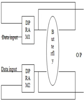
Single memory (pair) architecture (shown in Figure 2) is suitable for single snapshot applications, where samples are acquired and processed thereafter. The processing time is typically greater than the acquisition time. The main disadvantage in this architecture is while doing the transform process we cannot load the next coming data. We have to wait until the current data is processed. So we proposed dual memory (pair) architecture for faster sampling rate applications (shown in Figure 3). In this architecture there are three main processes for the transformation of the sampled data. Loading the sampled data into the memories, processing the loaded data, reading out the processed data. As there are two pairs of dual port memories available, one pair can be used for loading the incoming sampled data, while at the same time the other pair can be used for processing the previously loaded sampled data. For further sampling rate improvements we proposed multiple memory (pair) architecture (shown
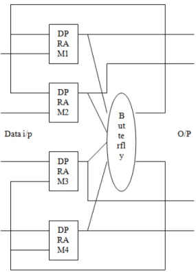
in Figure 4). This is the best of all architectures in case of very high sampling rate applications, but in case of hardware utilization it uses lot more resources than any other architecture. In this model there is a memory set, one arithmetic unit for each iteration. The advantage of this model over the previous models is that we do not need to wait until the end of all iterations (i.e. whole FFT process), to take the next set of samples to get the FFT process to be started again. We just need to wait until the end of the first iteration and then load the memory with the next set of samples and start the process again. After the first iteration the processed data is transferred to the next set of RAMs, so the previous set of RAMs can be loaded with the next coming new data samples. This leads to the increased sampling rate.
Coming to the implementation of the paired transform based DFT algorithm, there is no complete butterfly operation, as that in case of radix-2 algorithm. According to the mathematical description given in the Section II, the arithmetic unit is divided into two parts, addition part and multiplication part. This makes the main difference between the two algorithms, which causes the process of the DFT completes earlier than the radix-2 algorithm. The addition part of the algorithm for 8-point transform is shown in Figure 5.
The SIMULINK model diagrams for butterfly operation for both FFTs are given below.
75 (b)
Figure 1: SIMULINK models (a) for butterfly diagram for N=8 Cooley-Tukey FFT (b) for the
addition part (shown in figure 5) of Paired transform based FFT: Grigorayn FFT.
The architectures are implemented for the 8-point, 64-point, and 128-point transforms for Virtex-4 FPGAs. The radix-2 FFT algorithm is efficient in case of resource utilization and the paired transform algorithm is very efficient in case of higher sampling rate applications.
4.
Preliminary Implementation
Results
Results obtained on Virtex-4 FPGAs: The hardware
modeling of the algorithms is done by using Xilinx’s
system generator plug-in software tool running under SIMULINK environment provided under the Mathworks’s MATLAB software. The functionality of the model is verified using the SIMULINK Simulator and the MODELSIM software as well. The implementation is done using the Xilinx project navigator backend software tools.
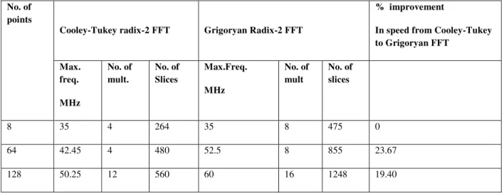
Table 1 shows the implementation results of the two algorithms on the Virtex-4 FPGAs. From the table we can see that Grigoryan FFT is always faster than the Cooley-Tukey FFT algorithm. Thus paired-transform based algorithm can be used for higher sampling rate applications. In military applications, while doing the process, only some of the DFT coefficients are needed at a time. For this type of applications paired transform can be used as it generates some of the coefficients earlier, and also it is very fast.
From the Reference 4 of IEEE paper (8 and 64 point FFT) we can be able to prove the same with Xilinx Virtex-II Pro FPGAs also. The results along with 128 point FFT also given in Table 2.
5.
Conclusions and Further Research
In this paper we have shown that with our FFT processors architectures on Xilinx Virtex-4 FPGAs the paired transform based Grigoryan FFT algorithm is faster and can be used at higher sampling rates than the Cooley-Tukey FFT at an expense of high resource utilization. Which is also in accordance with Virtex-II Pro FPGAs implementation in the reference number 4 IEEE paper, and we can be able to prove it one more time with Virtex-4 FPGAs also. As part of future research we are implementing for N = 256 point FFTs also. We are utilizing the MAC engines explicitly of TMS DSP processors for evaluating on
DSP processors also. We are developing a “neural
data acquisition and processing and RF wireless
transmitting” VLSI DSP processor where we will be
utilizing our Grigoryan FFT processors.
76
Figure 3: Dual memory (pair) architecture
Figure 4: Multiple memory (pair) architecture (Transform length = N = 2n)
(1,2);(3,4);(5,6) ---- (-,-) memory pairs for each iteration.
--- Butterfly unit for each iteration.
x1,0
x1,1
x1,2
x1,3
x2,0
x2,2
x4,0
x0,0
x(0)
x(1)
x(2)
x(3)
x(4)
x(5)
x(6)
x(7)
add operation
subtract operation
Figure 5: Figure showing the addition part of the 8-point paired transform based DFT
Acknowledgment
This is to acknowledge Dr. Parimal A. Patel, Dr. Artyom M. Grigoryan of The University of Texas at San Antonio for their valuable guidance for the first
part of this research series as Mr. Narayanam’s Master’s Thesis. Mr. Narayanam also would like to
acknowledge University of Ottawa research facility
References
[1] James W. Cooley and John W. Tukey, “An algorithm for the machine calculation of complex Fourier Series”, Math. comput. 19, 297-301 (1965).
[2] Artyom M. Grigoryan and Sos S. Agaian, “Split Manageable Efficient Algorithm for Fourier and Hadamard transforms Signal Processing, IEEE Transactions on, Volume: 48, Issue: 1, Jan.2000
Pages: 172 – 183.
[3] Virtex-4 Pro platform FPGAs: detailed
description
http://www.xilinx.com/support/documentation/da ta_sheets/ds112.pdf .
[4] Narayanam Ranganadh, Parimal A Patel and
Artyom M. Grigoryan, “Case study of Grigoryan
FFT onto FPGAs and DSPs”, IEEE proceedings,
ICECT – 2012.
[5] Smith, Steven W. "The scientist and engineer's
77
Table 1: Efficient performance of Grigoryan FFT over Cooley-Tukey FFT, on Virtex-4 FPGAs. Table showing the sampling rates and the resource utilization summaries for both the algorithms, implemented on the Virtex-4 FPGAs. We have utilized Extreme DSP slices in this, which is making us much faster than
Virtex-II Pro FPGAs.
Table 2: Efficient performance of Grigoryan FFT over Cooley-Tukey FFT, on Virtex-II Pro FPGAs. Table showing the sampling rates and the resource utilization summaries for both the algorithms, implemented on
the Virtex-II Pro FPGAs.
No. of points
Cooley-Tukey radix-2 FFT Grigoryan Radix-2 FFT
% improvement
In speed from Cooley-Tukey to Grigoryan FFT
Max. freq.
MHz
No. of mult.
No. of Slices
Max.Freq.
MHz
No. of mult
No. of slices
8 35 4 264 35 8 475 0
64 42.45 4 480 52.5 8 855 23.67
128 50.25 12 560 60 16 1248 19.40
No. of points Cooley-Tukey radix-2 FFT
Grigoryan Radix-2 FFT %
improvement In speed from Cooley-Tukey to Grigoryan FFT Max.
freq. MHz
No. of Slice s
No. of Extreme DSP slices
Max. freq MHz
No. of Slices
No.of Extreme DSP slices
78
Mr. Ranganadh Narayanam is an associate professor in the department of Electronics & Communications
Engineering in Aurora’s Scientific and Technological
Institute. Mr.Narayanam, was a research student in the area of “Brain Stem Speech Evoked Potentials” under the guidance of Dr. Hilmi Dajani of University of Ottawa,Canada. He was also a research student in The University of Texas at San Antonio under Dr. Parimal A Patel,Dr. Artyom M. Grigoryan, Dr Sos Again, Dr. CJ Qian,. in the areas of signal processing and digital systems, control systems. He worked in the area of Brian Imaging in University of California Berkeley. Mr. Narayanam has done some advanced learning in the areas of DNA computing, String theory and Unification of forces, Faster than the speed of light theory with worldwide reputed persons and world’s top ranked universities. Mr. Narayanam’s research interests include neurological Signal & Image processing, DSP software & Hardware design and implementations, neuro technologies.
Dr. Artyom M. Grigoryan received the MSs degree in mathematics from Yerevan State University (YSU), Armenia, USSR, in 1978, in imaging science from Moscow Institute of Physics and Technology, USSR, in 1980, and in electrical engineering from Texas A&M University, USA, in 1999, and Ph.D. degree in mathematics and physics from YUS, in 1990. In 1990-1996, he was a senior researcher with the Department of Signal and Image Processing at Institute for Problems of Informatics and Automation, and Yerevan State University, National Academy Science of Armenia. In 1996-2000 he was a Research Engineer with the Department of Electrical Engineering, Texas A&M University. In December 2000, he joined the Department of Electrical Engineering, University of Texas at San Antonio, where he is currently an Associate Professor. He holds two patents for developing an algorithm of automated 3-D fluorescent in situ hybridization spot counting and one patent for fast calculating the cyclic convolution. He is the author of three books, three book-chapters, two patents, and many journal papers and specializing in the theory and application of fast one- and multi-dimensional Fourier transforms, elliptic Fourier transforms, tensor and paired transforms, unitary heap transforms, design of robust linear and nonlinear filters, image enhancement, encoding, computerized 2-D and 3-D tomography, processing biomedical images, and image cryptography.