doi:10.5194/npg-17-481-2010
© Author(s) 2010. CC Attribution 3.0 License.
in Geophysics
Characterizing the nonlinear internal wave climate
in the northeastern South China Sea
S. R. Ramp1, Y. J. Yang2, and F. L. Bahr1
1Monterey Bay Aquarium Research Institute, 7700 Sandholdt Road, Moss Landing, CA, 95039, USA 2Department of Marine Science, Naval Academy, P.O. Box 90175, Kaohsiung 813, Taiwan
Received: 8 May 2010 – Accepted: 9 August 2010 – Published: 29 September 2010
Abstract. Four oceanographic moorings were deployed in the South China Sea from April 2005 to June 2006 along a transect extending from the Batanes Province, Philippines in the Luzon Strait to just north of Dong-Sha Island on the Chinese continental slope. The purpose of the array was to observe and track large-amplitude nonlinear internal waves (NIWs) from generation to shoaling over the course of one full year. The basin and slope moorings observed velocity, temperature (T) and salinity (S) at 1–3 min intervals to observe the waves without aliasing. The Luzon mooring observed velocity at 15 min andT andSat 3 min, primarily to resolve the tidal forcing in the strait.
The observed waves travelled WNW towards 282–288 degrees with little variation. They were predominantly mode-1 waves with orbital velocities exceeding 100 cm s−1 and thermal displacements exceeding 100 m. Consistent with earlier authors, two types of waves were observed: the a-waves arrived diurnally and had a rank-ordered packet structure. The b-waves arrived in between, about an hour later each day similar to the pattern of the semi-diurnal tide. The b-waves were weaker than the a-waves, usually consisted of just one large wave, and were often absent in the deep basin, appearing as NIW only upon reaching the continental slope. The propagation speed of both types of waves was 323±31 cm s−1 in the deep basin and 222±18 cm s−1 over the continental slope. These speeds were 11–20% faster than the theoretical mode-1 wave speeds for the observed stratification, roughly consistent with the additional contribution from the nonlinear wave amplitude. The observed waves were clustered around the time of the spring tide at the presumed generation site in the Luzon Strait, and no waves were observed at neap tide. A remarkable feature was the distinct lack of waves during the winter months, December 2005 through February 2006.
Correspondence to: S. R. Ramp
Most of the features of the wave arrivals can be explained by the tidal variability in the Luzon Strait. The near-bottom tidal currents in the Luzon Strait were characterized by a large fortnightly envelope, large diurnal inequality, and stronger ebb (towards the Pacific) than flood tides. Within about±4 days of spring tide, when currents exceeded 71 cm s−1, the ebb tides generated high-frequency motions immediately that evolved into well-developed NIWs by the time they reached mooring B1 in the deep basin. These waves formed diurnally and correspond to the a-waves described by previous authors. Also near spring tide, the weaker flood tides formed NIWs which took longer/further to form, usually not until they reached mooring S7 on the upper continental slope. These waves tracked the semidiurnal tide and correspond to the b-waves described by previous authors. These patterns were consistent from March to November. During December–February, the structure of the barotropic tide was unchanged, so the lack of waves during this time is attributed to the deep surface mixed layer and weaker stratification along the propagation path in winter.
1 Introduction
are favorable, the internal tide steepens and becomes more nonlinear, ultimately spawning packets of high-frequency internal solitary waves (hereafter ISWs). Two generating mechanisms are most commonly cited for the ISWs: 1) Lee waves, in the form of a strong depression of the thermocline, are trapped in the lee of a ridge on ebb tide and are released when the tide turns. The waves rapidly steepen and form ISWs as the bulge propagates in the direction of the flood tide (Maxworthy, 1979; Turner, 1973; Apel et al., 1985; Vlasenko and Alpers, 2005). If the flow across the ridge is hydraulically supercritical, the lee wave is replaced by a hydraulic jump in the lee of the ridge, with similar effect when the tide turns. Supercritical flows over a sill may also generate upstream ISWs (Cummins et al., 2003). 2) Internal tidal energy, initially in the form of vertically propagating beams, is trapped in the main thermocline by reflection and refraction (Akylas et al., 2007; Shaw et al., 2009; Buijsman et al., 2010a). The waves become increasingly 2-D and steepen downstream, ultimately forming ISWs when the particle speeds exceed the free wave propagation speed. Both processes are closely related to the strength of the tidal flow and the stratification at the generating site. The processes may not be mutually exclusive, with both making a contribution to the wave generation problem. These theoretical ideas have been nicely summarized recently in (Helfrich and Melville, 2006).
One location where ISWs are particularly clear and energetic is the northeastern South China Sea. Both synthetic aperture radar (Liu et al., 1998, 2004; Hsu and Liu, 2000) and ocean color (Kao et al., 2007) images have shown well-defined fields of ISWs propagating WNW across the sea from west of Luzon Strait to the Chinese continental shelf. The radar data reveal that the ISWs are depression waves in the open sea, changing to elevation waves in depths less than about 120–150 m on the continental shelf (Hsu and Liu, 2000). Most of the waves fit the expected surface signatures for mode-1 waves, but mode-2 waves have also been observed occasionally (Yang et al., 2004, 2009). The collective sea surface imagery suggests a few curious features. First, there seems to be a distinct lack of eastward-propagating waves on the Pacific side of the Luzon Ridge. This has recently been attributed to asymmetries in the tidal flux, thermal structure, and bottom topography across the ridge (Buijsman et al., 2010b) although observations on the Pacific side are lacking. Second, westward-propagating features generally do not appear in the surface imagery until a point west of the western (Heng-Chun) Ridge. This suggests that the Heng-Chun Ridge plays some role in the wave generation process. While this may be the case (Chao et al., 2007; Buijsman et al., 2010b) others have successfully modeled this result without the presence of a western ridge (Shaw et al., 2009; Zhang, 2010). Both show that the nonlinear internal tide requires a finite time to steepen to the point where ISWs develop on the leading edge of the bore, at a distance which approximately coincides with the location
west of the Heng-Chun Ridge where the surface signatures first appear. Again, in-situ observations sufficient to support these theoretical studies have been lacking.
Detailed observations of the ISW arrivals on the Chinese continental shelf over a full spring/neap tidal cycle were provided by the Asian Seas International Acoustics Exper-iment (ASIAEX), a cooperative experExper-iment between the US and Taiwan (Ramp et al., 2003, 2004; Orr and Mignerey, 2003; Duda et al., 2004b). Thermocline displacements exceeding 150 m which caused temperature changes at 100 m depth exceeding 8◦C were observed during the spring tides. The orbital velocities in the waves exceeded 150 cm s−1 with vertical velocities exceeding 50 cm s−1. Histograms of the wave phase speed and propagation direction showed that the largest and fastest waves were all traveling WNW towards 282◦N with speeds of around 150 cm s−1. This direction traces back directly to the center of the Luzon Strait, suggesting that the waves originated there, where the barotropic to baroclinic energy conversion is among the largest in the world (Niwa and Hibiya, 2004; H. Simmons, personal communication, 2009). The ASIAEX results were limited however by the experiment’s short duration (April 2001) and the complete lack of any observations in the deep basin or at the supposed generation site. Comparing the wave arrivals lagged back to the theoretical (modeled) Luzon Strait tide suggested correlation with the spring/neap tidal cycle in the strait, but individual waves could not be attributed to a specific beat of the theoretical tide. In a subsequent re-analysis of the same data set, other authors found that the waves were likely released from the Luzon Strait on the westward (flood) tide (Zhao and Alford, 2006). However, their analysis suffered from the same lack of observations as the original work, and used theoretical estimates for both the propagation speed of the waves and the beat of the tidal currents in the Luzon Strait. An error of only about 3% (10 cm s−1) in the propagation speed over 475 km from S7 to Luzon would be sufficient to cause the generation time to jump 6 h from a flood peak to an ebb peak. Given further that the precise location of the generation site was unknown, and that the model tidal currents were unverified, their determination of the phase relation between the barotropic tide and the release of the ISWs in Luzon Strait must be regarded as tentative.
117 118 119 120 121 122 123 18
19 20 21 22 23
−6000 −5000 −4000 −3000 −2000 −1000 0
Longitude (deg W)
La
titude (deg N)
Kaohsiung
S7 B1
B2 L1
Luzon
Mooring CTD
Taiwan
Batan Is.
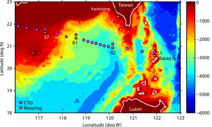
Fig. 1. Map showing asset locations during the WISE/VANS experiment from April 2005 to June 2006 in the South China Sea. The background color indicates bottom depth according to the color bar at right. The Batan Islands are on the eastern (Luzon) Ridge and the ridge south of Taiwan is the western (Heng-Chun) Ridge.
high-resolution observations of temperature (T), salinity (S), and velocity (u, v) at all four sites allowed unambiguous wave characterization and tracking between moorings. CTD transects conducted every three months observed the seasonal variation of the stratification along the propagation path. The rest of this manuscript describes the results from this program, with special attention placed on understanding the wave arrival patterns at each of the moorings across the sea over the course of the four seasons. The data and methods are described next, followed by the results, discussion, and conclusions.
2 Data and methods
The four moorings were deployed in water depths of 350 m (S7), 2460 m (B1), 3300 m (B2), and 460 m (L1) from west to east, respectively (Fig. 1). Mooring S7 (Fig. 1) could be described as an upper continental slope location and was at the same location as mooring S7 during the ASIAEX 2001 experiment. Moorings B1 and B2 were located in the deep basin away from abrupt topography. Mooring L1 was located on the side of a seamount in the channel between Batan and Itbayat Islands in the Luzon Strait. These islands are located on the Luzon Ridge, the more eastern of the two primary ridges in the Luzon Strait. While not optimal, the L1 location was dictated by the depth limitation (500 m) of the instrumentation available and could not be located on the sill (735 m) between the islands. The primary goal of L1 in any case was to observe the barotropic component of the tide, rather than any NIW motions. Toward that end, an upward-looking 300 kHz ADCP mounted in a cage 4 m off the bottom sampled 4-m bins every 15 min from 25 April until 28 October 2005, and then again from 28 October until the batteries expired on 11 May 2006. Additionally, the mooring also supported two temperature-conductivity-pressure (TCP) recorders and three temperature-temperature-conductivity-pressure
(TP) recorders. These instruments sampled at 3-min intervals for two months, with some programmed to start recording two and four months into the deployment so that a three-minute time series could be obtained for 6 months. These instruments provided some indication of the high-frequency variability near the mooring which turned out to be quite useful. The pressure sensors on these instruments mostly recorded mooring motion, however the deepest pressure sensor mounted on the acoustic release with minimal motion sampled a pressure record that was well correlated with a tide gauge deployed at Basco Pier, located about 10 km away in the capital city of the Batanes Province on Batan Island.
The basin and slope moorings required 1-min sampling to avoid aliasing the high frequency motions of interest. This dictated using four 3-month deployments to obtain a full year’s worth of data due to battery life and internal memory constraints. Using lessons learned from the ASIAEX program, mooring S7 used double steel spheres at the top and a 4000 lb anchor to reduce mooring blow-down when the ISWs passed by. Velocity was sampled via a cage mounted, upward-looking 300 kHz ADCP at 103 m depth, and three conventional ducted-paddlewheel and vane current meters moored nominally at 163 m, 223 m, and 313 m depth. The stratification and thermal displacements induced by the ISWs were sampled by 4 TCP and 8 TP recorders distributed along the mooring wire from 35 m depth to 12 m off the bottom. This mooring configuration was used from April to July 2005 and again from November 2005 to February 2006. For the 3-month deployment in between and for the final three months, a simpler mooring configuration was used with an upward-looking 150 kHz ADCP mounted in a syntactic foam float at 250 m depth, just one TCP recorder at 260 m, and a single current meter at 303 m. While this mooring sampled temperature and salinity less well, it served to better define the zero (modal crossing) point in the velocity.
The basin moorings were a logistical challenge due to their length and the strong currents experienced from the internal waves, internal tides, and occasionally the mesoscale circulation. At mooring B1, the upward-looking 300 kHz ADCP was mounted in a 49′′syntactic foam sphere at 100 m depth, and a second very large (64′′) sphere at 760 m depth provided additional buoyancy. A hard plastic fairing was attached to the jacketed wire rope in the upper water column to reduce drag. Heavy biofouling on this substrate during the first deployment likely made the situation worse, but there was subsequently no biofouling at all during the remaining three deployments. Two TCP and eight TP recorders spread out along the mooring line observed the temperature and salinity displacements. The locations and time histories of these and all other instruments in the experiment are summarized in Table 1.
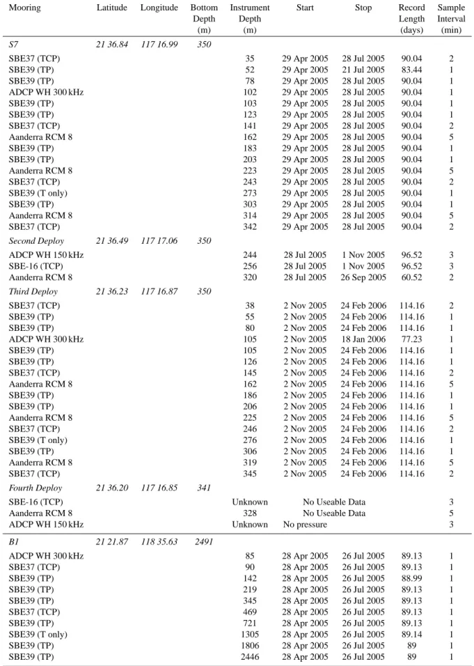
Table 1. Mooring and instrument locations for the four deployments in the South China Sea.
Mooring Latitude Longitude Bottom Instrument Start Stop Record Sample
Depth Depth Length Interval
(m) (m) (days) (min)
S7 21 36.84 117 16.99 350
SBE37 (TCP) 35 29 Apr 2005 28 Jul 2005 90.04 2
SBE39 (TP) 52 29 Apr 2005 21 Jul 2005 83.44 1
SBE39 (TP) 78 29 Apr 2005 28 Jul 2005 90.04 1
ADCP WH 300 kHz 102 29 Apr 2005 28 Jul 2005 90.04 1
SBE39 (TP) 103 29 Apr 2005 28 Jul 2005 90.04 1
SBE39 (TP) 123 29 Apr 2005 28 Jul 2005 90.04 1
SBE37 (TCP) 141 29 Apr 2005 28 Jul 2005 90.04 2
Aanderra RCM 8 162 29 Apr 2005 28 Jul 2005 90.04 5
SBE39 (TP) 183 29 Apr 2005 28 Jul 2005 90.04 1
SBE39 (TP) 203 29 Apr 2005 28 Jul 2005 90.04 1
Aanderra RCM 8 223 29 Apr 2005 28 Jul 2005 90.04 5
SBE37 (TCP) 243 29 Apr 2005 28 Jul 2005 90.04 2
SBE39 (T only) 273 29 Apr 2005 28 Jul 2005 90.04 1
SBE39 (TP) 303 29 Apr 2005 28 Jul 2005 90.04 1
Aanderra RCM 8 314 29 Apr 2005 28 Jul 2005 90.04 5
SBE37 (TCP) 342 29 Apr 2005 28 Jul 2005 90.04 2
Second Deploy 21 36.49 117 17.06 350
ADCP WH 150 kHz 244 28 Jul 2005 1 Nov 2005 96.52 3
SBE-16 (TCP) 256 28 Jul 2005 1 Nov 2005 96.52 3
Aanderra RCM 8 320 28 Jul 2005 26 Sep 2005 60.52 2
Third Deploy 21 36.23 117 16.87 350
SBE37 (TCP) 38 2 Nov 2005 24 Feb 2006 114.16 2
SBE39 (TP) 55 2 Nov 2005 24 Feb 2006 114.16 1
SBE39 (TP) 80 2 Nov 2005 24 Feb 2006 114.16 1
ADCP WH 300 kHz 105 2 Nov 2005 18 Jan 2006 77.23 1
SBE39 (TP) 105 2 Nov 2005 24 Feb 2006 114.16 1
SBE39 (TP) 126 2 Nov 2005 24 Feb 2006 114.16 1
SBE37 (TCP) 145 2 Nov 2005 24 Feb 2006 114.16 2
Aanderra RCM 8 162 2 Nov 2005 24 Feb 2006 114.16 5
SBE39 (TP) 186 2 Nov 2005 24 Feb 2006 114.16 1
SBE39 (TP) 206 2 Nov 2005 24 Feb 2006 114.16 1
Aanderra RCM 8 225 2 Nov 2005 24 Feb 2006 114.16 5
SBE37 (TCP) 246 2 Nov 2005 24 Feb 2006 114.16 2
SBE39 (T only) 276 2 Nov 2005 24 Feb 2006 114.16 1
SBE39 (TP) 306 2 Nov 2005 24 Feb 2006 114.16 1
Aanderra RCM 8 319 2 Nov 2005 24 Feb 2006 114.16 5
SBE37 (TCP) 345 2 Nov 2005 24 Feb 2006 114.16 2
Fourth Deploy 21 36.20 117 16.85 341
SBE-16 (TCP) Unknown No Useable Data 3
Aanderra RCM 8 328 No Useable Data 5
ADCP WH 150 kHz Unknown No pressure 3
B1 21 21.87 118 35.63 2491
ADCP WH 300 kHz 85 28 Apr 2005 26 Jul 2005 89.13 1
SBE37 (TCP) 90 28 Apr 2005 26 Jul 2005 89.13 1
SBE39 (TP) 142 28 Apr 2005 26 Jul 2005 88.99 1
SBE39 (TP) 219 28 Apr 2005 26 Jul 2005 89.13 1
SBE39 (TP) 345 28 Apr 2005 26 Jul 2005 89.13 1
SBE37 (TCP) 469 28 Apr 2005 26 Jul 2005 89.13 1
SBE39 (TP) 721 28 Apr 2005 26 Jul 2005 89.13 1
SBE39 (T only) 1305 28 Apr 2005 26 Jul 2005 89.14 1
SBE39 (TP) 1806 28 Apr 2005 26 Jul 2005 89 1
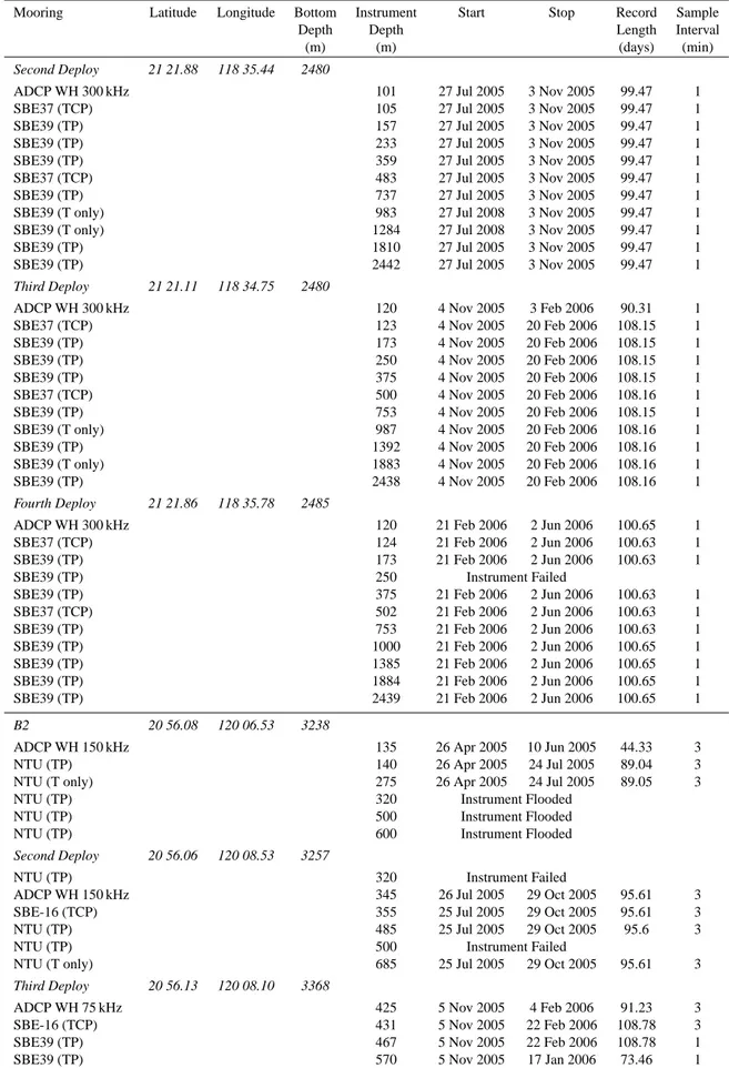
Table 1. Continued.
Mooring Latitude Longitude Bottom Instrument Start Stop Record Sample
Depth Depth Length Interval
(m) (m) (days) (min)
Second Deploy 21 21.88 118 35.44 2480
ADCP WH 300 kHz 101 27 Jul 2005 3 Nov 2005 99.47 1
SBE37 (TCP) 105 27 Jul 2005 3 Nov 2005 99.47 1
SBE39 (TP) 157 27 Jul 2005 3 Nov 2005 99.47 1
SBE39 (TP) 233 27 Jul 2005 3 Nov 2005 99.47 1
SBE39 (TP) 359 27 Jul 2005 3 Nov 2005 99.47 1
SBE37 (TCP) 483 27 Jul 2005 3 Nov 2005 99.47 1
SBE39 (TP) 737 27 Jul 2005 3 Nov 2005 99.47 1
SBE39 (T only) 983 27 Jul 2008 3 Nov 2005 99.47 1
SBE39 (T only) 1284 27 Jul 2008 3 Nov 2005 99.47 1
SBE39 (TP) 1810 27 Jul 2005 3 Nov 2005 99.47 1
SBE39 (TP) 2442 27 Jul 2005 3 Nov 2005 99.47 1
Third Deploy 21 21.11 118 34.75 2480
ADCP WH 300 kHz 120 4 Nov 2005 3 Feb 2006 90.31 1
SBE37 (TCP) 123 4 Nov 2005 20 Feb 2006 108.15 1
SBE39 (TP) 173 4 Nov 2005 20 Feb 2006 108.15 1
SBE39 (TP) 250 4 Nov 2005 20 Feb 2006 108.15 1
SBE39 (TP) 375 4 Nov 2005 20 Feb 2006 108.15 1
SBE37 (TCP) 500 4 Nov 2005 20 Feb 2006 108.16 1
SBE39 (TP) 753 4 Nov 2005 20 Feb 2006 108.15 1
SBE39 (T only) 987 4 Nov 2005 20 Feb 2006 108.16 1
SBE39 (TP) 1392 4 Nov 2005 20 Feb 2006 108.16 1
SBE39 (T only) 1883 4 Nov 2005 20 Feb 2006 108.16 1
SBE39 (TP) 2438 4 Nov 2005 20 Feb 2006 108.16 1
Fourth Deploy 21 21.86 118 35.78 2485
ADCP WH 300 kHz 120 21 Feb 2006 2 Jun 2006 100.65 1
SBE37 (TCP) 124 21 Feb 2006 2 Jun 2006 100.63 1
SBE39 (TP) 173 21 Feb 2006 2 Jun 2006 100.63 1
SBE39 (TP) 250 Instrument Failed
SBE39 (TP) 375 21 Feb 2006 2 Jun 2006 100.63 1
SBE37 (TCP) 502 21 Feb 2006 2 Jun 2006 100.63 1
SBE39 (TP) 753 21 Feb 2006 2 Jun 2006 100.63 1
SBE39 (TP) 1000 21 Feb 2006 2 Jun 2006 100.65 1
SBE39 (TP) 1385 21 Feb 2006 2 Jun 2006 100.65 1
SBE39 (TP) 1884 21 Feb 2006 2 Jun 2006 100.65 1
SBE39 (TP) 2439 21 Feb 2006 2 Jun 2006 100.65 1
B2 20 56.08 120 06.53 3238
ADCP WH 150 kHz 135 26 Apr 2005 10 Jun 2005 44.33 3
NTU (TP) 140 26 Apr 2005 24 Jul 2005 89.04 3
NTU (T only) 275 26 Apr 2005 24 Jul 2005 89.05 3
NTU (TP) 320 Instrument Flooded
NTU (TP) 500 Instrument Flooded
NTU (TP) 600 Instrument Flooded
Second Deploy 20 56.06 120 08.53 3257
NTU (TP) 320 Instrument Failed
ADCP WH 150 kHz 345 26 Jul 2005 29 Oct 2005 95.61 3
SBE-16 (TCP) 355 25 Jul 2005 29 Oct 2005 95.61 3
NTU (TP) 485 25 Jul 2005 29 Oct 2005 95.6 3
NTU (TP) 500 Instrument Failed
NTU (T only) 685 25 Jul 2005 29 Oct 2005 95.61 3
Third Deploy 20 56.13 120 08.10 3368
ADCP WH 75 kHz 425 5 Nov 2005 4 Feb 2006 91.23 3
SBE-16 (TCP) 431 5 Nov 2005 22 Feb 2006 108.78 3
SBE39 (TP) 467 5 Nov 2005 22 Feb 2006 108.78 1
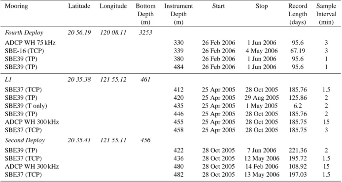
Table 1. Continued.
Mooring Latitude Longitude Bottom Instrument Start Stop Record Sample
Depth Depth Length Interval
(m) (m) (days) (min)
Fourth Deploy 20 56.19 120 08.11 3253
ADCP WH 75 kHz 330 26 Feb 2006 1 Jun 2006 95.6 3
SBE-16 (TCP) 339 26 Feb 2006 4 May 2006 67.19 3
SBE39 (TP) 380 26 Feb 2006 1 Jun 2006 95.6 1
SBE39 (TP) 484 26 Feb 2006 1 Jun 2006 95.6 1
L1 20 35.38 121 55.12 461
SBE37 (TCP) 412 25 Apr 2005 28 Oct 2005 185.76 1.5
SBE39 (TP) 420 25 Apr 2005 29 Aug 2005 125.86 2
SBE39 (T only) 435 25 Apr 2005 1 May 2005 6.2 2
SBE39 (TP) 446 25 Apr 2005 28 Oct 2005 185.76 2
ADCP WH 300 kHz 455 25 Apr 2005 28 Oct 2005 185.75 15
SBE37 (TCP) 458 25 Apr 2005 28 Oct 2005 185.75 3
Second Deploy 20 35.41 121 55.11 456
SBE39 (TP) 422 28 Oct 2005 7 Jun 2006 221.36 2
SBE37 (TCP) 436 28 Oct 2005 12 May 2006 195.72 1.5
ADCP WH 300 kHz 480 28 Oct 2005 14 Feb 2006 108.92 15
SBE37 (TCP) 482 28 Oct 2005 13 May 2006 197.03 1.5
were deployed between 265 and 800 m to observe the stratification. The rest of the mooring below 800 m consisted of double-plaited nylon line and distributed buoyancy. For the second half of the experiment, the ADCP at 250 m was replaced by a 75 kHz ADCP at 500 m, with two TP recorders at 550 m and 650 m. The performance of these instruments is also shown in Table 1.
During all five deployment and recovery cruises, CTD stations were conducted from the research vessel OCEAN RESEARCHER 1, owned and operated by National Taiwan University. The instrument was lowered at 60 m/min through the upper 500 m and 100 m/min thereafter. The primary purpose of the CTD stations was to allow computation of the linear wave speed across the basin. The sections also revealed the position of the Kuroshio intrusion and several large mesoscale eddies, and described the seasonal variability of the surface mixed layer and thermocline depth. The latter two features turned out to be quite important to understanding the seasonal variability of the high-frequency internal wave field in the northeastern South China Sea.
3 Results
3.1 Wave properties
The evolution of the NIWs from east to west is first discussed referencing the temperature and velocity signatures of some prototypical wave forms as they passed moorings B2, B1, and S7 (Fig. 2). The waves shown are a typical example from 17–19 November 2005, near spring tide. These waves
were similar in form and evolution to waves observed at other times during March–November. This description focuses on wave evolution during westward propagation: The issue of wave generation will be discussed subsequently. At B2, located just west of the Heng-Chun Ridge, the waves were indistinct in both temperature and velocity and resembled a nonlinear internal tide more than a soliton. The broad thermal depression from 12:00–13:00 on 17 November was accompanied by a westward upper layer velocity exceeding 100 cm s−1. The wave took about an hour to pass by the mooring. An energetic but incoherent internal wave field was visible in the temperature plot, but not in the velocity plot, possibly due to the lower resolution and broad sampling swath of the 75 kHz ADCP. This may also be due to beam spreading of the ADCP relative to the geophysical wavelength being observed, especially in the layers most distant from the transducer heads (Scotti et al., 2005). There was no recognizable high-frequency wave on the previous tidal beat spanning 01:00–03:00.
Fig. 2. Stack plots of (left) east-west velocity component and (right) temperature at moorings B2 (top), B1 (middle), and S7 (bottom) during
17–19 November 2005. The x-axes have been chosen to show the same soliton passing by, approximately aligned vertically. Speed and temperature scales are shown by the color bars.
in the lead wave. Since this velocity plot shows only the upper 120 m, only the westward (upper layer) velocities are evident. A new feature appeared at B1 between 1600–1800 in both velocity and temperature. These features coincide temporally with the weaker beat of the tide between 0100– 0300 at mooring B2. This feature now resembled a nonlinear tide and represents the beginnings of the second NIW which appeared subsequently at mooring S7.
Upon arrival at mooring S7, the disturbances observed at B1 had morphed into five NIWs with clear signatures in both temperature and velocity (bottom panel). Four of these waves evolved from the original group of two at B1, and the fifth represents the nonlinear evolution of the weaker tidal beat, which appeared only as a tide at B1. In keeping with earlier work (Ramp et al., 2004) these waves have been labeled with a lower case a and b to denote the a-waves and b-waves they described. The two largest waves a1 and a2 dispersed slightly, consistent with the larger amplitude a1 wave traveling about 6% faster than the smaller a2 wave. This is approximately consistent with the nonlinear (KdV) theory. A new wave labeled a1′also appeared at S7, located between a1 and a2. This wave was likely spawned by the lead wave a1 as it shoaled from 2465 to 350 m depth, as there were many other examples of this in the record when the lead wave was large. The origin of the a3 wave is unknown: it could have evolved from one of the smaller
5 10 15 20 25 30
00:00 03:00 06:00 09:00 12:00 15:00 18:00 21:00 24:00
500
1000
1500
2000
B1 Temperature May 25
Pressure (db)
Time (hours UTC)
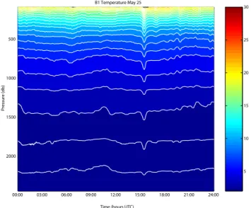
Fig. 3. Temperature contour plot of a large solitary wave passing
mooring B1 on 25 May 2005. The color bar is at the right and selected isotherms have been highlighted in white.
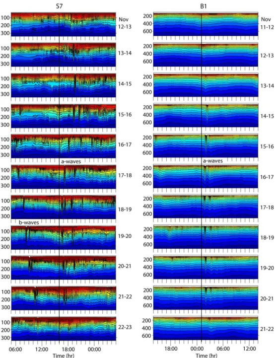
Fig. 4. Daily stack plots of temperature at B1 (right) and S7 (left) during 11–23 November 2005. The plots have been offset vertically by
one day to account for the travel time between moorings, so that the same wave is depicted in the same horizontal panel of each column. A comparison of the right and left panels therefore shows the wave evolution from B1 to S7. The a- and b-wave arrivals are labeled. The vertical lines are a visual aid for aligning the wave arrivals.
B1. All these waves at S7 were mode-1 waves with a first crossing (zero-point) located at around 130–140 m depth. The wave velocities above this point were westward with an eastward return flow below. The westward velocities again approached 150 cm s−1while the deeper currents towards the east maxed out at around 100 cm s−1.
closely related issues of propagation speed and travel time are taken up in greater detail subsequently, for this figure it suffices to know that the travel time for each wave from B1 to S7 was approximately 15 h (136 km at 2.5 m s−1). Thus, there is no ambiguity in terms of which wave at B1 resulted in the corresponding wave packets at S7. Working from the top of the plot to the bottom shows how the wave field evolved from neap tide to spring tide and back to neap tide again. Describing first the arrival patterns at B1, there were no waves at all observed during 11–12 November. Starting on 13 November, the strongest waves arrived diurnally like clockwork at B1 at about 02:00 every day. The first hint of a wave appeared on 13 November, grew stronger on 14–15 November, and was then followed by several very large waves arriving during 16–21 November. During this time the waves were usually observed as packets of two with little variation in amplitude from day to day. On the morning of 22 November, the waves disappeared once again, ending the fortnightly cycle. The sudden appearance and disappearance of the waves suggests some critical condition at the generation site which must be met to generate and sustain the waves, an idea which is revisited again in the discussion section. Starting at 14:30 on 15 November and arriving 55 min later each day, there was a second, much weaker “bump” in the isotherms that indicated a nonlinear internal tide, but no well defined NIW appeared on the weaker tidal beat at the B1 location.
The upstream conditions at B1 resulted in a profusion of wave arrivals by the time the waves reached site S7 (Fig. 4, left panel). When the initial conditions were very weak, at or near neap tide, no NIW ever formed even at S7, as for instance on 12–13 and 22–23 November (top and bottom panel, respectively). Features which resembled nonlinear tides at B1, such as the a-wave on 13–14 November and the b-waves during 15–21 November, became well-developed NIWs at S7. Waves which were already well developed at B1 became multi-wave packets at S7. The a-wave arrivals at S7 were still diurnal but with slightly more variation in arrival time than at site B1. The larger waves generated closer to the spring tide during 17–22 November arrived at S7 about 1–2 h earlier than the three previous days. This order 5% change in propagation speed could be attributed to their greater nonlinear wave amplitude, but might also be due to the mesoscale circulation advancing or retarding the wave arrivals. The b-wave arrivals were delayed each day approximately consistent with the semidiurnal tidal progression, and consisted of just one or two waves per packet. The b-wave amplitude at S7 however was often just as large as the leading a-waves.
3.2 Propagation speed
To further characterize the propagation speed of the NIWs, individual waves (or nonlinear internal tidal peaks which ultimately became waves) were tracked between moorings
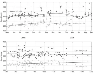
Fig. 5. Observed and computed propagation speeds of the nonlinear
waves as a function of (a) time and (b) non-linear wave amplitude
(positive downward). The observed propagation speeds were
computed by tracking the waves between moorings B2 and B1 (black dots) and B1 and S7 (gray dots). The heavy black and gray lines in the upper panel show the 6th order polynomial fit to the data. The mean values and standard deviations are also shown. The theoretical mode-1 linear phase speeds (triangles) were computed from the CTD data as described in the text.
using a cross-correlation method. The clearest wave signal was actually observed in the pressure time series, using the large increase which occurred when the mooring was blown down each time a large NIW passed by. As such, the pressure signal was a proxy for velocity, but acted as a natural filter and produced a cleaner signal with a higher signal-to-noise ratio. Large internal solitary waves pushed the mooring down a lot, whereas random linear internal wave activity with shorter vertical correlation scales pushed it down very little. Very similar results were obtained by correlating temperature fluctuations at a standard depth. The procedure used was to subset 1-day windows around each wave peak and slide the two time series (B2 and B1, then B1 and S7) until the maximum correlation was reached. This time lag produced the time necessary for the wave to propagate between the two moorings. As a sanity check, each result was visually inspected by an expert to be sure the computer was not correlating with some incorrect or spurious peak. Only clear results were kept: With so many realizations to use over the 13-month time series, any doubtful or marginal peaks were simply thrown out and not used in the results presented.
observations (Alford et al., 2010; Klymak et al., 2006). The large offset between the B2 to B1 speeds and B1 to S7 was primarily due to the changing bottom depth. Moorings B2 and B1 were both in the deep basin where the bottom depth decreased gently from 3300 to 2465 m, whereas the bottom shoaled from 2465 to 350 m between B1 and S7. Aside from this offset there are several other features of note. At both locations, the propagation speed of the waves increased with the seasonal stratification during the spring and summer and then decreased during the winter when the mixed layer deepened and stratification weakened. From B1 to S7, propagation speed was a weak function of nonlinear wave amplitude, according to the equation
Cp=211+0.128η
Thus, 120 m waves were 5% faster than 40 m waves, approximately consistent with similar waves observed in the Sulu Sea (Apel et al., 1985). Interestingly, the propagation speed vs. nonlinear wave amplitude curves for B2 to B1 were statistically flat, indicating no relationship between amplitude and propagation speed in deep water. This is perhaps because the waves at B2 were not yet steep enough to display a clear relationship between propagation speed and nonlinear wave amplitude.
Also shown on the figure are triangles indicating the linear phase speed for the mode-1 waves, computed using the CTD data for each of the five deployment/recovery cruises. The mode-1 phase speeds were computed for each CTD station (Fig. 1) as a solution to the Sturm-Liouville equation governing the vertical motions in a non-rotating, hydrostatic, zero-shear fluid with wave frequency much higher than the inertial frequency (Apel et al., 1985, 1997; Alford et al., 2010).
d2Wn
dz2 + N2(z)
c2
n
Wn=0
Subject to the boundary conditions Wn(0)=Wn(−H )=0
The theory further suggests that the linear and nonlinear phase speeds for each mode are related by:
Cn=cn+
αnηn
3
whereCnis the nonlinear (KdV) phase speed,cnis the linear
phase speed,ηis the nonlinear wave amplitude,αdepends on the stratification, and n is the mode number.
The linear phase speeds shown in Fig. 5 for each season were computed as the weighted average of the mode-1 speeds between each mooring pair, calculated using all available CTD data between the moorings. The annual changes in the linear phase speeds thus computed were small, ranging from 260–277 cm s−1 in the deep basin and 191 to 209 cm s−1 over the continental slope. The computed speeds showed
2005/6 2005/8 2005/10 2005/12 2006/2 2006/4 2006/6 0
50 100 150
2005/6 2005/8 2005/10 2005/12 2006/2 2006/4 2006/6
0 50 100 150 200
2005/6 2005/8 2005/10 2005/12 2006/2 2006/4 2006/6 0
100 200 300 400
t (db
)
emen
m Displac
o Isother
15
olit
on Speed (cm/s)
S
tion (deg)
ec
on Dir
olit
S
Mooring B1
Mean=53±27
Mean=42±24
Mean=47±30
Mean=39±26
Mean=288±31
Mean=282±24
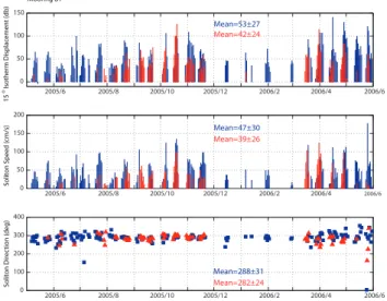
Fig. 6. A compendium of nonlinear wave characteristics as they
passed mooring B1 from May 2005 to June 2006. The amplitudes
based on the displacement of the 15◦C isotherm (top panel),
maximum upper layer orbital velocities as sensed by the ADCP (middle panel) and directions (bottom panel) are shown for the a-waves (blue) and the b-a-waves (red).
the same weak trends as the data, i.e. increasing with the stratification from May to August and decreasing from August to November. The linear mode-1 phase speeds were 11–20% slower than suggested by the observed wave travel times from B2 to B1 and 9–23% slower from B1 to S7. This is consistent with earlier observations (Alford et al., 2010) and the theory described above.
Seasonal variation of wave arrivals
0 50 100 150 0
5 10 15 20 25 30
5 10
15 30
210
60
240
90 270
120 300
150 330
180 0
0 50 100 150
0 5 10 15 20 25 30
5 10
15 30
210
60
240
90 270
120 300
150 330
180 0
S7 B1
Speed (cm/s)
C
oun
ts
C
oun
ts
Direction (deg)
Fig. 7. Histograms of wave orbital velocity and direction for mooring B1 (top) and mooring S7 (bottom).
282–288◦N. The a-waves and b-waves were classified by careful inspection of the data, aka Fig. 4. On average, the a-waves were 11 m larger, 8 cm s−1 faster, and angled 6◦ further towards the north than the b-waves at site B1.
Histograms of wave speed and direction were constructed for moorings S7 and B1 using the high-pass filtered velocity data for the entire record (Fig. 7). Direction was determined as the direction of the upper layer velocity, whose speed was calculated as the vector sum of the u- and v-components. The primary wave direction at S7 was towards the WNW or 282◦N, similar to the same location during spring 2001 (also 282◦) (Ramp et al., 2004). The direction histograms were remarkably similar at B1, towards 288◦N for the a-waves and 282◦N for the b-waves. Neither site shows any hint of large reflected waves going the opposite direction: The waves must instead be refracted along the gradual continental slope. A computation of the internal wave ray slope indicates that it is always shallower than the local continental slope, leading to forward scattering only. The wave current speed histograms at B1 and S7 were remarkably similar. The most common upper layer orbital velocities were in the 30– 35 cm s−1range, with maxima just over 100 cm s−1.
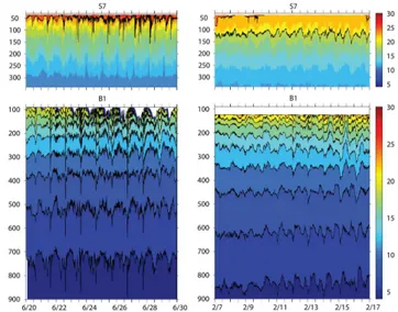
An important result is the distinct absence of waves during the winter, from December 2005 to February 2006. To understand this result, the thermal stratification and number of NIW occurrences were compared for 20–30 June, 2005 and 7–07 February 2006 (Fig. 8). Both time periods were centered on a spring tide. During the summer, the June picture (left panel) is entirely consistent with Figure 4 showing large diurnal NIW arrivals at B1 and both diurnal and semidiurnal packets arriving at S7. During February however, when the tidal forcing in the Luzon Strait was similar, a vigorous internal tide persisted but no NIWs
Fig. 8. Temperature contours for mooring S7 (top) and B1 (bottom)
for a) 20–30 June 2005 and (b) 7–17 February 2006 showing wave occurrences vs. stratification. The black line at S7 during
June highlights the 24◦C isotherm. The other black line at S7 in
February tracks the 20◦C isotherm.
were observed passing B1 or S7. A significant difference between the two panels is the surface mixed layer depth (MLD), which was less than 50 m in summer but greater than 100 m in winter. Despite the low latitude, the sea surface temperature exhibited an 8◦ seasonal change from just over 30◦in summer to about 22◦in winter. This cooling in addition to the increased wind stress during the winter monsoon fosters the deeper MLD in winter.
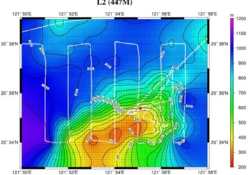
Fig. 9. Detail of the bottom topography near mooring L1 (red dot)
based on a ship survey (white line) conducted from the Research
Vessel OCEAN RESEARCHER 1. The seamount pictured is
located in the gap between Batan and Itabayat Island (Fig. 1). Contours outside the sampling pattern have been extrapolated and have low confidence.
of February) can in fact be rigorously correlated with brief re-stratification events, which can be attributed to warm spells and passing mesoscale eddies. Thus it is difficult, but not impossible, for NIWs to form in winter.
3.3 Currents at L1
So far this paper has focused on describing the wave arrivals at various points as they propagate WNW across the South China Sea. Attention is now focused on the currents, temperature, and pressure observed at mooring L1 in the Luzon Strait, and how these fluctuations might be related to the features ultimately observed far downstream. To properly interpret these observations, a more detailed view of the mooring location relative to abrupt topography is needed. The mooring was located on a steep slope on the side of a seamount rising from 1000 m to less than 300 m in the gap between Batan and Itbayat Island (Figs. 1, 9). This gap was chosen for the observations because: 1) Ray tracing from the other moorings points to this location as the source; and 2) numerical models show this location to be one of the areas with maximal barotropic to baroclinic tidal energy conversion (Niwa and Hibiya, 2004). For reasons still unclear, the range of the 300 kHz ADCP was nominally 70 m, sometimes even less, rather than the usual 110 m. The instrument’s automatic gain control and correlation magnitude indicate the instrument was receiving no signal beyond this range. This would suggest extraordinarily clear water in the area with no scatterers. The CTD fluorometer showed no chlorophyll below 200 m. Unfortunately a beam transmissometer was not deployed. The result of the limited range of the instrument was that the volume sampled was
−100 0 100 200
−100 0 100 200
0 50 100 150 200
u (cm/s)
v (cm/s)
Speed (cm/s)
Apr May Jun Jul Aug Sep Oct Nov Dec Jan Feb
Apr May Jun Jul Aug Sep Oct Nov Dec Jan Feb
Apr May Jun Jul Aug Sep Oct Nov Dec Jan Feb
2005 2006
Fig. 10. The u-component (top), v-component (middle) and total
speed (bottom) at 420 m depth (40 m off the bottom) at mooring
L1 in the Luzon Strait. Positive (negative)uis towards the Pacific
(South China Sea) side and represents the ebb (flood) tide. Positive
(negative)vis towards the north (south) and represents the flood
(ebb) tide. The lunar cycle is indicated across the top of the plot, with hollow circles indicating the time of the full moon and solid circles the new moon.
all well below the summit of the seamount, and represents a small fraction (15%) of the water column near the bottom.
Fig. 11. The east-west (a) and north-south (b) current components
for one fortnightly cycle of currents at mooring L1 in the Luzon Strait. The temperature (c) and east-west component (d) for 25 May 2005 are expanded in the two panels below. White spaces indicate missing or bad data.
represent clockwise tidal rectification around the seamount (Loder et al., 1997; Lee and Beardsley, 1999; H. Simmons, personal communication, 2009). There was no sign of the Kuroshio flowing through this passage at any time. The CTD data and personal shipboard observations showed the Kuroshio to be flowing northward over the western ridge, i.e., it loops around the central Batan Islands (Centurioni and Niiler, 2004; Liang et al., 2008). Also shown across the top of the plot are the times of the new and full moon (Fig. 10). Correlation of the lunar cycle with the currents in the strait shows that spring tides were not phase locked to the lunar cycle. A rigorous tidal analysis (Table 2) shows that this was because the fortnightly beat resulted from the interplay of the M2, K1, O1, and much weaker S2 tidal constituents, rather than just the M2 and S2 as is more commonly observed. The tides could be categorized as mixed, diurnal dominant, and were diurnal near spring tide and semidiurnal at neap tide.
The tidal structure can be seen in much greater detail if a single fortnightly cycle is expanded showing all the data (Fig. 11). The tides were semidiurnal from 17 to 21 May becoming diurnal on 24–28 May. The tides look remarkably uniform, but with no data from the upper water column one cannot say definitively if these plots represent barotropic or baroclinic flow. Correlations between the vertically averaged east-west component with the tidal height at Basco were visually identical with a normalized cross-correlation coefficient of 0.88. This strongly suggests that the observed high tide was coherent with flood tide at L1, i.e. mostly barotropic. Furthermore, the vertically-averaged currents at L1 were used to calculate fifty-one tidal constituents, which were used to reconstruct the tide and project it into the future for comparison with another mooring during April– July 2007 which had data from the upper water column. The phases of the currents were precisely aligned, again
Table 2. Ellipse parameters for the vertically averaged tidal
currents.
In order of magnitude
Consti- Major Minor Inclination Phase SNR
tuent (cm/s) (cm/s) (From N) (degrees)
M2 40.34 1.04 106 346 1500
K1 28.25 –4.48 94 124 420
O1 26.15 –5.13 95 94 360
S2 15.08 –0.10 107 14 210
N2 7.71 1.09 109 334 55
P1 7.57 –2.34 102 136 31
Q1 6.09 –1.26 97 83 20
MSF 5.28 0.34 78 37 16
MF 4.20 –1.65 77 254 10
suggesting that the L1 mooring was observing mostly the barotropic tide.
There was a temporal asymmetry in the flow as well, especially at spring tide: a typical pattern, evident in Fig. 11a and expanded for 25 May in the lower panel (Fig. 11d), consisted of a strong eastward flow (red) from 04:00 to 10:00, followed by eleven hours of dead water from 11:00 to 22:00, followed by a shorter, weaker westward flow from 23:00 to 02:00. This unusual pattern was repeated near spring tide throughout the record. The strong tides pumped cold water up the flank of the seamount, especially on the stronger ebb tide (Fig. 11c). Nearby CTD stations show that the ambient depth of the 6◦C water that appeared for instance at 07:30 on 25 May was about 650 m. The tide thus forced a vertical excursion of order 200 m in the local isotherms as it pumped back and forth across the seamount.
Fig. 12. High-pass filtered data from mooring L1. The top three
panels are the u-, v-, and w-components from bin 8, approximately 422 m depth (39 m off the bottom). The bottom pressure series is from the instrument mounted just below the top sphere at 410 m depth.
centered on the time of the spring tides (7 and 21 July). These fluctuations exceeded the background noise and were of order plus or minus 15–20 cm s−1. The cleanest signal was in the pressure record from just below the top sphere at 410 m depth (Fig. 12d). These pressure fluctuations were due to mooring blow-down and are thus a proxy for velocity, but sampled at 3-min intervals rather than 15. The pressure record was not aliased by internal waves and captured all the high frequency events. It appears that random fields of internal waves did not push down the mooring, which only responded to the more vertically coherent structures. Below a certain threshold, the mooring did not respond at all, resulting in a very clear visual indicator of the time when coherent high frequency motions occurred. These signals were observed clustered around the time of the spring tide throughout the entire year. Their distinctive shape was tractable between moorings and allowed considerable information regarding wave generation to be gained.
4 Discussion
4.1 Relating downstream waves to the L1 tides
The high-passed pressure fluctuations from all the moorings plotted together show how the waves evolved as they propagated WNW across the sea (Fig. 13). As the waves propagated, the central peak in the pressure fluctuation grew larger and the side lobes became smaller until only a single downward spike remained at S7. This downward pressure spike was perfectly correlated with the wave-induced velocity and temperature fluctuations. The travel
0 6 12 18 0 6 12 18 0 6 12 18 0 6 12 18 0
0 10 20 30
P (db)
0 6 12 18 0 6 12 18 0 6 12 18 0 6 12 18 0
−2 0 2 4 6
0 6 12 18 0 6 12 18 0 6 12 18 0 6 12 18 0
−10 0 10
0 6 12 18 0 6 12 18 0 6 12 18 0 6 12 18 0
−2 0 2 4
P (db)
P (db)
P (db)
August 19 August 20 August 21 August 22 S7
B1
B2
L1 136 km
174 km
184 km 18.93 hr = 2.7 m/s
14.21 hr = 3.4 m/s 17.17 hr = 2.2 m/s
Fig. 13. High-pass filtered pressure fluctuations at moorings S7
(top), B1 (upper middle), B2 (lower middle), and L1 (bottom) for 19–22 August 2005. The distances and travel time between moorings are indicated.
times computed using this method are identical to the statistical mean (Fig. 5) from B1 to S7 and within 2 cm s−1 from B2 to B1. The waves required 33.1 h to propagate from L1 to B1, and 50.3 h (2.1 days) to travel from L1 to S7. This is much less than the 3.7 days estimated using continental slope data alone (Ramp et al., 2004). Those authors had no data from the deep basin and did not appreciate how much faster the waves travel there. It is also 7.3 h faster than the 57.6 h estimated by comparing the ASIAEX data set against model currents at Luzon, using historical CTD data to estimate the stratification and mode speeds along the path (Zhou and Alford, 2006).
These precise estimates of the travel time make it possible to rigorously correlate wave arrivals at B1 with a specific tidal beat in the Luzon Strait, using observations only. A representative example for the month of August 2005 (Fig. 14) shows the wave arrivals at B1 lagged back by 33 h, plotted over the L1 tide, which was reconstructed using the full suite of tidal constituents from the Foreman analysis. The lagged a-wave arrivals at B1 line up precisely with the peak ebb tide at L1 (Fig. 14, dotted lines). This result is consistent with the NLIWI 2007 data (Alford et al., 2009) but contrasts with earlier work that suggested that the waves were formed on the flood tide (Zhao and Alford, 2006). This is easy to understand given that the ZA06 estimate of the travel time (57 vs. 50 h) was off by half a semidiurnal tidal cycle.
−50 0 50 100
11 12 13 14 15 16 17 18 19 20 21 22 23 24 25 −100
−50 0 50 100 150
11 12 13 14 15 16 17 18 19 20 21 22 23 24 25 −3
−2 −1 0 1 2 3 4
15
oC Isotherm depth (db)
u (cm/s)
Pressure (db)
August 2005
L1 High Pass B1
L1 Tide
11 12 13 14 15 16 17 18 19 20 21 22 23 24 25
Fig. 14. The 15◦C isotherm displacements at mooring B1, lagged back 33 h to account for the propagation time from mooring L1 to B1 (top). The Foreman reconstruction of the tidal currents at mooring L1, using the vertically averaged data (middle). The high-passed pressure data from mooring L1, 410 m depth (bottom). The vertical dotted lines indicate the time of a-wave arrivals at mooring B1, and the dashed lines are the b-wave arrivals. The horizontal
lines on the middle panel indicate plus or minus 71 cm s−1.
a-waves were observed at mooring B1. This 71 cm s−1 threshold was consistent across all the data obtained, and suggests that a critical speed in the strait is necessary for these high-frequency fluctuations and downstream NIWs to form. This argument would be more correctly cast in terms of a Froude number (U/c1), but unfortunately the stratification data needed to estimate the mode-1 free wave speed (c1) for the water column at L1 was not obtained during this experiment. Quantitatively relating wave formation to the Froude number in the strait remains a subject of future research.
On the other hand, the b-waves at B1 were aligned perfectly with the flood tide at L1, and were not associated with a local high-frequency pressure fluctuation in the strait (Fig. 14, dashed lines). This contrasts with earlier authors who thought the b-waves formed on the weaker beat of the ebb tide, and took longer in both space and time to steepen due to the lower Froude number on formation (Ramp et al., 2004; Zhang, 2010). The different timing, the weaker flood tides, the lack of an associated high-frequency pressure fluctuation for the b-waves, and the different packet structure downstream all suggest different generation mechanisms or perhaps even different generation locations for the a-waves and b-waves. These ideas may be illuminated by recent theory, and this is taken up in the next section.
4.2 Comparisons with the SUNTANS model
In a companion paper (Zhang et al., 2010) hereafter referred to at ZFR10, the parallel, unstructured grid, nonhydrostatic ocean model SUNTANS (Fringer, 2006) was used to simulate the wave generation process during 17–30 June 2005 for comparison with the WISE/VANS observed results. The model used a variable grid with 1– 4 km resolution, 100 vertical layers, and an 11-s time step, and required 7 days of wall-clock time to perform the 14-day simulation. The model provides some insight into the three-dimensional variability which is not available from a two-dimensional observational transect. ZFR10 found two important generation sites in the Luzon Strait, one near L1 between Batan and Itbayat Island, and another further south on the eastern ridge near 19◦30′N, 122◦00′E. In the model, both sites generated both a- and b-waves, but the northern site (near L1) was more efficient for b-waves and the southern site better for a-waves. The difference lies in the topography: The bottom slope is closer to critical for the semidiurnal tide at the northern site and for the diurnal tide at the southern site. Tidal resonance at the M2 frequency between the two ridges at the northern site also enhances the b-wave formation there. As a result of the two locations, the a-waves (282◦) propagate more northerly than the b-waves (267◦). The model also shows that the a-waves originate on the ebb tide and the b-waves at the flood tide. In a closely related work, the SUNTANS model also shows that downstream evolution of the nonlinear internal waves in both space and time is a close function of the Froude number at generation (Zhang, 2010). Larger waves appear sooner and closer to the source when the Froude number at the source is large. When the barotropic tide, and thus the Froude number, falls below a certain value, no waves are formed. These model results are all in good qualitative agreement with the observational results reported here. Additional more focused field programs are needed to make more quantitative comparisons.
The actual generation mechanisms remain a bit less clear. ZFR10 show that the a-waves result from the generation of diurnal internal tidal beams at critical topography, especially in the southern portion of the eastern ridge, where the west ridge is quite deep and effectively absent. The situation for the b-waves is less obvious, as it is confused by the complicated resonant region between the two ridges where standing waves and higher mode internal waves may exist. The SUNTANS model produces weaker tidal beams for the b-waves in this region. ZFR10 hypothesize that the b-waves are tidally generated during peak flood tides in a manner similar to (Buijsman et al., 2010).
beam-forming and nonlinear steepening (Shaw et al., 2009; Zhang, 2010; Buijsman et al., 2010a, b) but inconsistent with the observed a-waves which had an associated high-frequency signature immediately in the strait. The a-wave formation seems consistent with a lee wave mechanism, although the observations on the Pacific side of the strait are insufficient to show this. We suggest that east of 120◦30′E, the waves are likely too weakly nonlinear for their orbital velocities to reach the surface and create signatures that can be detected by MODIS or a SAR. The waves near mooring B2 were only weakly nonlinear, with orbital velocities less than 50 cm s−1 and propagation speeds exceeding 320 cm s−1. This combination of a very fast-moving wave with relatively weak orbital velocities is unfavorable for surface slick formation. Further to the west at S7 and B1, the waves slow down and the orbital velocities speed up, until on the upper continental slope (ASIAEX moorings S7 to S5, Ramp et al., 2004) the two are about equal at 150 cm s−1. These conditions seem ideal to form surface convergences and divergences and very strong slicks and bands of breaking waves, which are easily detectable by satellite. Waves formed near the bottom in 735 m of water (sill depth) require a finite distance to travel along ray paths before they strike the surface and manifest themselves there. This distance also corresponds roughly to 120◦30′E. Another possibility is that the observed high frequency fluctuations at the time of a-wave generation are actually smaller-scale features associated with the flow over a seamount, and do not contribute to the basin-wide phenomenon. In this case it would just be coincidence that these features appeared at same time as the a-wave generation.
5 Conclusions
Moored observations of temperature, salinity, and velocity were obtained at 1–5 min intervals from April 2005–June 2006 to resolve the seasonal variability of the nonlinear internal wave field in the northeastern South China Sea. Three moorings spanned the sea, with two in the deep basin and one on the upper continental slope. A fourth mooring in the Luzon Strait, designed primarily to document the barotropic tide, sampled velocity at 15-min intervals and T, S, and P at three-minute intervals. Hydrographic (CTD) transects along the mooring line were obtained on all five cruises to document seasonal changes to the stratification along the wave propagation path.
On the upper slope, two types of waves, called a-waves and b-a-waves, were observed in keeping with earlier work. The a-waves arrived diurnally and consisted of rank-ordered packets, while the b-waves arrived an hour later each day and usually had a single large wave extending from the middle of a group of smaller waves. While the b-waves appeared to track the semidiurnal tide, they appeared just once per day. Both wave types traveled
WNW at mooring S7 and were in all respects similar to the same location during the ASIAEX experiment. The a-waves were also present further “upstream” at B1 and were easily traceable between moorings. The b-waves however were much weaker or absent entirely at mooring B1 and only became fully developed at S7. Very large amplitude waves were formed year-round except during December– February when almost no waves were observed. Continuing further towards the source, both wave types at mooring B2 more closely resembled highly nonlinear internal tides than high-frequency internal waves. Still, these distinctive wave forms could in most cases be followed between the basin moorings to estimate propagation speeds. The propagation speeds were first and foremost a function of the total water depth, and secondarily functions of stratification and nonlinear wave amplitude. The waves on average travelled at 323±31 cm s−1between B2 and B1, and at 222±18 cm s−1 between B1 and S7, which was about 10–20% faster than the linear mode-1 internal wave speed based on the observed stratification. The waves traveled towards 282◦ for the b-waves and 288◦for the a-waves.
Most of the variability in the wave arrival patterns at the moorings was directly attributable to variability in the barotropic tidal currents in the Luzon Strait. The tides were mixed diurnal dominant, with a strong diurnal inequality that produced nearly diurnal tides at spring tide and semidiurnal at neap. The fortnightly beat in the strait was very large ranging from <50 cm s−1 at neap tide to >200 cm s−1at spring tide. Nonlinear internal waves were only generated within plus or minus about 4 days of spring tide and were absent otherwise. The cutoff was very sharp, i.e. transitioning from no waves to huge waves in a single tidal cycle with no intermediate-sized waves being formed. This suggests some critical value in the strait which must be exceeded for NIWs to form. Using a thirty-three hour propagation time between moorings L1 and B1 shows that the a-waves were generated on the much stronger ebb tide while the b-waves corresponded to the weaker flood tide. The ebb tide also generated high-frequency fluctuations in velocity and pressure immediately in the strait while the flood tide did not. The absence of waves in the winter is attributed to changes in the stratification along the propagation path, with the deeper surface mixed layer and weaker upper ocean stratification suppressing wave formation in the winter.
present in the strait, the suddenness with which the transition from the no-waves to waves state takes place, and the immediate formation of high-frequency fluctuations on the peak ebb tide, the formation of lee waves cannot be ruled out. Clearly some additional field observations focused on the generation region are warranted to establish the relative importance of the various generation mechanisms.
Acknowledgements. A field program of this size cannot be
achieved without the dedication and hard work of many individuals. Professors Wen-Ssn Chuang (NTU) and Ching-Sang Chiu (NPS) led the February 2006 cruise. The moorings and instruments were expertly prepared, deployed, and recovered by Wen-Hwa Her (NTU) and Marla Stone (NPS) who sailed on all five cruises. A cadre of six or more graduate students per cruise (NTU) worked tirelessly on deck without complaint. The officers and crew of the Research Vessel OCEAN RESEARCHER I (Taiwan) skillfully supported operations on all five cruises. This work was supported by the National Science Council (NSC, Taiwan) and the Office of Naval Research (ONR, USA).
Edited by: K. Helfrich
Reviewed by: T. Duda and another anonymous referee
References
Akylas, T. R., Grimshaw, R. H. J., Clarke, S. R., and Tabaei, A.: Reflecting tidal wave beams and local generation of solitary waves in the ocean thermocline, J. Fluid Mech., 593, 297–313, 2007.
Alford, M. H., Lien, R.-C., Simmons, H., Klymak, J., Ramp, S. R., Yang, Y. J., Tang, T.-Y., Farmer, D., and Chang, M.-H.: Speed and evolution of nonlinear internal waves transiting the South China Sea, J. Phys. Oceanogr., 40(6), 1338–1355, doi: 10.1175/2010JPO4388.12010, 2010.
Apel, J. R., Holbrook, J. R., Liu, A. K., and Tsai, J.: The Sulu Sea internal soliton experiment, J. Phys. Oceanogr., 15, 1625–1651, 1985.
Apel, J. R., Badiey, M., Chiu, C.-S., Finette, S., Headrick, R., Kemp, J., Lynch, J. R., Newhall, A., Orr, M. H., Pasewark, B. H., Tielbuerger, D., von der Heydt, K., and Wolf, S.: An overview of the 1995 SWARM shallow-water internal wave acoustic scattering experiment, IEEE J. Oceanic Eng., 22, 465– 500, 1997.
Armi, L. and Farmer, D. M.: The flow of Mediterranean water through the Strait of Gibraltar, Prog. Oceanogr., 21, 1–105, 1988. Bole, J. B., Ebbesmeyer, C. C., and Romea, R. D.: Soliton currents in the South China Sea: Measurements and theoretical mod-elling, in: Proc. 26th Annual Offshore Technology Conference (OTC), Houston, TX, USA, 367–376, 1994.
Buijsman, M. C., Kanarska, Y., and McWilliams, J. C.: On
the generation and evolution of nonlinear internal waves in the South China Sea, J. Geophys. Res.-Oceans, 115, C02012, doi:10.1029/2009JC005275, 2010a.
Buijsman, M. C., McWilliams, J. C., and Jackson, C. R.: East-west asymmetry in nonlinear internal waves from Luzon Strait, J. Geophys. Res.-Oceans, submitted, 2010b.
Centurioni, L. R., Niiler, P. P., and Lee, D.-K.: Observations of inflow of Philippine Sea surface water into the South China Sea through the Luzon Strait, J. Phys. Oceanogr. 34, 113–121, 2004. Chao, S.-Y., Ko, D.-S., Lien, R.-C., and Shaw, P.-T.: Assessing the west ridge of Luzon Strait as an internal wave mediator, J. Oceanogr., 63, 897–911, 2007.
Chapman, D. C., Ko, D.-S., and Preller, R. H.: A high-resolution numerical modeling study of the subtidal circulation in the northern South China Sea, IEEE J. Oceanic Eng., 29, 1087–1104, 2004.
Chiu, C.-S., Ramp, S. R., Miller, C. W., Lynch, J. F., Duda, T. F., and Tang, T.-Y.: Acoustic intensity fluctuations induced by South China Sea internal tides and solitons, IEEE J. Oceanic Eng., 29, 1249–1263, 2004.
Colosi, J. A., Lynch, J. F., Beardsley, R. C., Gawarkiewicz, G., Scotti, A., and Chiu, C.-S.: Observations of nonlinear internal waves on the New England continental shelf during the summer Shelfbreak Primer study, J. Geophys. Res.-Oceans, 106, 9587– 9601, 2001.
Cummins, P. F., Vagle, S., Armi, L., and Farmer, D. M.: Stratified flow over topography: Upstream influence and generation of nonlinear internal waves, P. Roy. Soc. Lond. A Mat., 459, 1467– 1487, 2003.
Duda, T. F., Lynch, J. F., Irish, J. D., Beardsley, R. C., Ramp, S. R., Chiu, C.-S., Tang, T.-Y., and Yang, Y.-J.: Internal tide and nonlinear internal wave behavior at the continental slope in the northern South China Sea, IEEE J. Oceanic Eng., 29, 1105–1131, 2004a.
Duda, T. F., Lynch, J. F., Newhall, A. E., Wu, L., and Chiu, C.-S.: Fluctuation of 400-hz sound intensity in the 2001 ASIAEX South China Sea Experiment, IEEE J. Oceanic Eng., 29, 1264– 1279, 2004b.
Ebbesmeyer, C. C., Coomes, C. A., Hamilton, R. C., Kurrus, K. A., Sullivan, T. C., Salem, B. L., Romea, R. D., and Bauer, R. J.: New observations on internal waves (solitons) in the South China Sea using an acoustic Doppler current profiler, in: Proc. Marine Technology Society, New Orleans, LA, 165–175, 1991. Farmer, D. M. and Smith, J. D.: Tidal interaction of stratified flow
with a sill in Knight Inlet, Deep-Sea Res., 27A, 239–254, 1980. Farmer, D. M. and Armi, L.: The flow of Atlantic water through the
Strait of Gibraltar, Prog. Oceanogr., 21, 1–105, 1988.
Foreman, M. G. G.: Manual for tidal currents analysis and
prediction, Pacific Marine Science Report 78-6, Institute of Ocean Sciences, Patricia Bay, Sidney, BC, 57 pp., 1978.
Fringer, O. B., Gerritsen, M., and Street, R. L.: An
unstructured grid, finite-volume, nonhydrostatic, parallel
coastal ocean simulator, Ocean Model., 14, 139–278,
doi:10.1016/J.OCEMOD.2006.03.006, 2006.
Global Ocean Associates: An Atlas of Internal Solitary-like
Waves and Their Properties, 2nd edn., available at: http://www. internalwaveatlas.com/ (last access: September 2010), 2004. Helfrich, K. R. and Melville, W. K.: Long nonlinear internal waves,
Annu. Rev. Fluid Mech., 38, 395–425, 2006.
Hsu, M.-K. and Liu, A. K.: Nonlinear internal waves in the South China Sea, Can. J. Remote Sens., 26, 72–81, 2000.
Kao, C.-C., Lee, L.-H., Tai, C.-C., and Wei, Y.-C.: Extracting the ocean surface feature on non-linear internal solitary waves
in MODIS satellite images, in: The Third International
Conferences on Intelligent Information Hiding and Multimedia Signal Processing, Kaohsiung, Taiwan, 27–32, 2007.
Klymak, J. M., Pinkel, R., Liu, C.-T., Liu, A. K., and David, L.: Prototypical solitons in the South China Sea, Geophys. Res. Lett., 33, L11607, doi:10.1029/2006GL025932, 2006.
Lee, S.-H. and Beardsley, R. C.: Influence of stratification on residual tidal currents in the Yellow Sea, J. Geophys. Res.-Oceans, 104, 15679–15701, 1999.
Liang, W.-D., Yang, Y. J., Tang, T.-Y., and Chuang, W.-S.: Kuroshio in the Luzon Strait, J. Geophys. Res.-Oceans, 113, C08048, doi:10.1029/2007JC004609, 2008.
Lien, R.-C., Tang, T. Y., Chang, M. H., and D’Asaro, E. A.: Energy of nonlinear internal waves in the South China Sea. Geophys. Res. Let, 32, L05615, doi:10.1029/2004GL022012, 2005. Liu, A. K., Chang, Y. S., Hsu, M.-K, and Liang, N. K.: Evolution
of nonlinear internal waves in the East and South China Seas, J. Geophys. Res.-Oceans, 103, 7995–8008, 1998.
Liu, A. K., Ramp, S. R., Zhao, Y., and Tang, T.-Y.: A case study of internal solitary wave propagation during ASIAEX 2001, IEEE J. Oceanic Eng., 29, 1144–1156, 2004.
Loder, J. W., Shen, Y., and Ridderinkhof, H.: Characterization of three-dimensional Lagrangian circulation associated with tidal rectification over a submarine bank, J. Phys. Oceanogr. 27, 1729– 1742, 1997.
Mazzega, P. and Berg´e, M.: Ocean tides in the Asian semi-enclosed sea from TOPEX/POSEIDON, J. Geophys. Res.-Oceans, 99, 24867–24881, 1994.
Maxworthy, T.: A note on the internal solitary waves produced by tidal flow over a three-dimensional ridge, J. Geophys. Res.-Oceans, 84, 338–346, 1979.
Niwa, Y. and Hibiya, T.: Three-dimensional numerical simulation of the M2 internal tides generated around the continental shelf edge in the East China Sea, J. Geophys. Res.-Oceans, 109, C04027, doi:10.1029/2003JC001923, 2004.
Orr, M. H. and Mignerey, P. C.: Nonlinear internal waves in the South China Sea: Observation of the conversion of depression internal waves to elevation internal waves, J. Geophys. Res.-Oceans, 108(C3), 3064, doi:10.1029/2001JC001163, 2003.
Pawlowicz, R., Beardsley, R. C., and Lentz, S.: Classical tidal harmonic analysis including error estimates in MATLAB using T TIDE, Comput. Geosci., 28, 929–937, 2002.
Ramp, S. R., Lynch, J. F., Dahl, P. H., Chiu, C.-S., and Simmen, J. A.: Program fosters advances in shallow-water acoustics southeastern Asia, EOS T. Am. Geophys. Un., 84(37), 361-376, doi:10.1029/2003EO370001, 2003.
Ramp, S. R., Tang, T.-Y., Duda, T. F., Lynch, J. F., Liu, A. K., Chiu, C.-S., Bahr, F. L., Kim, H.-R., and Yang, Y. J.: Internal solitons in the northeastern South China Sea Part I: Sources and deep water propagation, IEEE J. Oceanic Eng., 29, 1157–1181, 2004. Scotti, A., Butman, B., Beardsley, R. C., Alexander, P. S., and Anderson, S.: A modified beam-to-earth transformation to measure short-wavelength internal waves with an acoustic Doppler current profiler, J. Atmos. Ocean. Tech., 22, 583–591, 2005.
Shaw, P.-T., Ko, D.-S., and Chao, S.-Y.: Internal solitary waves induced by flow over a ridge: With applications to the northern South China Sea, J. Geophys. Res.-Oceans, 114, C02019, doi:10.1029/2008JC005007, 2009.
Turner, J. S.: Buoyancy effects in fluids, Cambridge University Press, Cambridge, 368 pp., 1973.
Vlasenko, V. and Alpers, W.: Generation of secondary internal waves by the interaction of an internal solitary wave with an underwater bank, J. Geophys. Res.-Oceans, 110, C02019, doi:10.1029/2004JC002467, 2005.
Yang, Y. J., Tang, T.-Y., Chang, M. H., Liu, A. K., Hsu, M.-K., and Ramp, S. R.: Solitons northeast of Tung-Sha Island during the ASIAEX pilot studies, IEEE J. Oceanic Eng., 29, 1182–1199, 2004.
Yang, Y. J., Fang, Y. C., Chang, M.-H., Ramp, S. R., Kao, C.-C., and Tang, T.-Y.: Observations of second baroclinic mode internal solitary waves on the continental slope of the northern South China Sea, J. Geophys. Res.-Oceans, 114, C10003, doi:10.1029/2009JC005318, 2009.
Ye, A. L. and Robinson, I. S.: Tidal dynamics in the South China Sea, Geophys. J. Roy. Astron. Soc., 72, 691–707, 1983. Zhang, Z.: Numerical simulations of nonlinear internal waves in the
South China Sea, Ph.D. dissertation, Stanford University, USA, 178 pp, 2010.