Benchmarking and Analysis of
Store Performance in a Retail Group
Ana Catarina Lourenço Mendonça
Católica Porto Business School March 2019
Benchmarking and Analysis of
Store Performance in a Retail Group
Final work in Project modality submitted to Universidade Católica Portuguesa to obtain the Master’s Degree in Management (specialization in Business Analytics)
by
Ana Catarina Lourenço Mendonça
under the supervision of Professora Doutora Conceição Silva
Católica Porto Business School March 2019
“If you can measure it, you can manage it” Robert S. Kaplan
Acknowledgments
This dissertation has been, beyond question, one of the most challenging projects that I have undertook, for the commitment, rigor and dedication required, but also for the enriching journey. In fact, this project has brought me theoretical knowledge that I could apply in a real-life context, offering me a close perception of the firm’s activity.
First of all, my main and greatest acknowledgement goes to my supervisor Professor Conceição Silva, for accepting the supervision of this project and for helping and supporting me when things seem to be adverse. The guidance regarding the way forward in the development of the work and the knowledge transmitted to me during this period was of major importance for the accomplishment of the project.
Secondly, I would like to thank my family and my friends for the all the support, understanding and encouragement in this last step of my education.
And finally, I would like to express my deepest gratitude to my supervisor at DESFO, SA, Pedro Figueiredo, for allowing me to use DeBorla Group data in this study, for all the challenges proposed in order to make my project better and, above all, for the availability and continuous support of my decisions in this dissertation.
Abstract
An everyday need of retail firms operating in saturated markets, where they face fierce competition, is the accurate and unbiased analysis of store performance. The aim of this work is to analyse and benchmark store efficiency and propose targets for store performance improvement in a Portuguese Retail Group. Panel data for 27 stores in the period 2015 to 2017 has been used to allow the assessment of store efficiency and the setting of improvement goals for the inefficient units, while identifying adequate efficiency drivers.
The methodologies and literature review allowed the identification of the techniques to be applied in the study: 1) Data Envelopment Analysis, to measure stores relative efficiency and to set improvement targets to the stores under analysis; 2) Tobit Regression Model, to identify the predominant factors leading to efficiency. Literature review and analysis of the available dataset enabled the selection of the variables to be used when applying each of the above techniques.
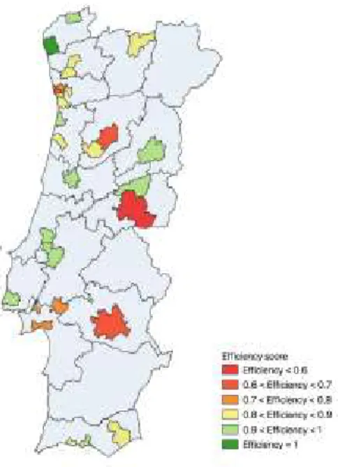
The work undertaken led to a number of important conclusions, regarding different aspects of this real life multivariable problem: 1) identification of efficient and inefficient stores; 2) store efficiency distribution by geographical location; 3) evolution of store efficiency over the time; 4) definition of performance targets for the inefficient stores; 5) benchmark highest performing units against lowest performing units with different indicators and 6) identification and quantification of the environmental factors influencing store efficiency.
Key-words: Store Performance, Store Efficiency, Retail Analytics, Retail Performance Benchmarking, Data Envelopment Analysis, Tobit Regression Model.
Resumo
As empresas de retalho que operam em mercados saturados, com uma concorrência feroz, têm a necessidade constante de fazer uma análise precisa e imparcial do desempenho das suas lojas. O objetivo deste trabalho é analisar e comparar a eficiência das lojas um grupo de retalho em Portugal propondo objetivos de melhoria de desempenho. Foram utilizados dados em painel para 27 lojas referentes ao período de 2015 a 2017, para avaliar a eficiência das lojas e estabelecer objetivos de melhoria para as unidades ineficientes, identificando também os fatores com maior impacto na eficiência.
As metodologias e a revisão de literatura permitiram a identificação das técnicas a aplicar no estudo: 1) Data Envelopment Analysis, para medir a eficiência relativa e definir objetivos de melhoria para as lojas em análise; 2) Tobit Regression Model, para identificar os fatores predominantes que conduzem à eficiência. A revisão de literatura e a análise da amostra disponível suportaram a seleção das variáveis a serem utilizadas na aplicação de cada uma das técnicas.
O trabalho realizado conduziu um conjunto de conclusões importantes, relativamente a diferentes aspetos deste problema real multivariável: 1) identificação das lojas eficientes e ineficientes; 2) distribuição da eficiência das lojas por localização geográfica; 3) evolução da eficiência das lojas ao longo do tempo; 4) definição de objetivos de desempenho para as lojas ineficientes; 5) Comparação das lojas de elevado e baixo desempenho relativamente a diferentes indicadores e 6) a identificação e quantificação das variáveis ambientais que afetam a eficiência.
Palavras-chave: Desempenho da loja, Eficiência da loja, Análise de retalho,
Comparação de desempenho no retalho, Data Envelopment Analysis, Tobit Regression
Index
Acknowledgments ... vii
Abstract... ix
Resumo ... xi
Index ... xiii
Index of Figures ...xvi
Index of Tables ... xvii
Acronyms ... xix
Chapter 1 - Introduction ... 21
1. Research objectives ... 22
2. Structure ... 23
Chapter 2 – The empirical setting ... 25
1. The firm - DESFO SGPS, S.A. ... 25
Chapter 3 – Methodologies ... 27
1. Data Envelopment Analysis (DEA) ... 27
1.1 Basic Formulations of the DEA Methodology ... 29
1.2 CCR and BCC models ... 31
1.3 Scale effects ... 34
2. Tobit Regression Model ... 36
Chapter 4 - Literature Review ... 39
1. Studies on retail performance ... 39
2. DEA applied to the benchmark of retail stores ... 41
2.1 Factors that influence performance ... 44
Chapter 5 – Description of the store set and dataset ... 47
1. Contextualization and description of the stores in the dataset ... 47
Chapter 6 - Store Performance Evaluation ... 55
1. Selection of variables ... 56
2. Identification of the Return to Scale type ... 58
3. Identification of the inefficiency sources ... 58
4. Efficiency Results assuming VRS without environmental variables ... 59
5. Comparative analysis of individual store performance ... 61
6. Store performance over time ... 64
7. Performance improvement goals without environmental variables ... 66
8. Benchmarking highest performing units against lowest performing units70 Chapter 7 - Impact of the environmental variables on store efficiency ... 75
Chapter 8 - Conclusions ... 81
1. Results ... 81
2. Contributions and Future Work ... 83
References ... 85
Appendix ... 89
Appendix A - Attach to Chapter 4 ... 89
Appendix B - Attach to Chapter 5 ... 91
B.1 Values of the variable “population within the trade area” for each DeBorla store (in millions of people) ... 91
B.2 Values of the average distance travelled to each DeBorla Store ... 92
B.3 Number of stores of each competitor within the trade area ... 93
B.4 Store distance to the nearest competitor ... 94
Appendix C - Attach to Chapter 6 ... 95
C.1 DEA model results without environmental variables for all 71 observations ... 95
C.2 DEA model efficiency results, assuming VRS, without environmental variables, for all 27 stores ... 98
C.3 DEA model benchmarks results, assuming VRS, without environmental variables... 99
C.4 Performance improvement goals according to DEA model without
environmental variables, assuming VRS ... 101 C.5 Percentage of potential gains according to DEA model without
environmental variables assuming VRS ... 105 C.6 Characterization of each of all 27 stores regarding their District,
Index of Figures
Figure 1 – CRS and VRS frontiers according to (Banker et al., 1984) ... 35
Figure 2 - Locations and respective surrounding areas for each DeBorla store ... 50
Figure 3 - Population within the trade area ... 51
Figure 4 - Locations of DeBorla stores and their customers ... 52
Figure 5 - Location of DeBorla stores (red) and competitors stores (green) ... 53
Figure 6 – Store efficiency distribution with VRS ... 60
Figure 7 -Average efficiency ranking of all the stores analysed ... 61
Figure 8 – Location of DeBorla stores according to their average efficiency... 63
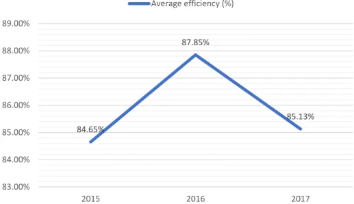
Figure 9 - Average store efficiency between 2015-2017 ... 64
Figure 10 - Potential gain of each variables (aggregate values for all the stores) ... 67
Figure 11 - Radar graph with inputs and outputs of the highest and lowest performing units ... 71
Figure 12 - Matrix positioning the top performance units and bottom performance units ... 73
Figure 13 - Radar graph with General Store Costs, Salaries, Sales, EBITDA and EBITDA margin for the highest and lowest performing units ... 74
Figure 14 – Impact on efficiency of the environmental variables -benchmarking top with bottom performers ... 78
Index of Tables
Table 1 - Categorization of variables of the dataset ... 48
Table 2 - Detail of the variables that compose the dataset ... 49
Table 3 - Comparison between average distance and median distance travelled by customers ... 52
Table 4 - Correlation matrix supporting the selection of discretionary variables .. 57
Table 5 - Mean and median of the discretionary variables of the DEA model ... 57
Table 6 - Technical inefficiency sources for all observations ... 59
Table 7 - Summarized Statistics of Store Efficiency observations ... 60
Table 8 – Average stores efficiency by region ... 62
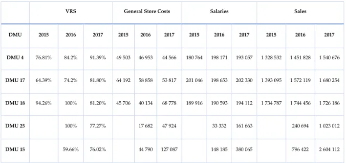
Table 9 –Score efficiency, General Store Costs, Salaries and Sales values for selected stores ... 65
Table 10 - Potential reductions of inputs and potential increases of output (aggregate values for all stores) ... 67
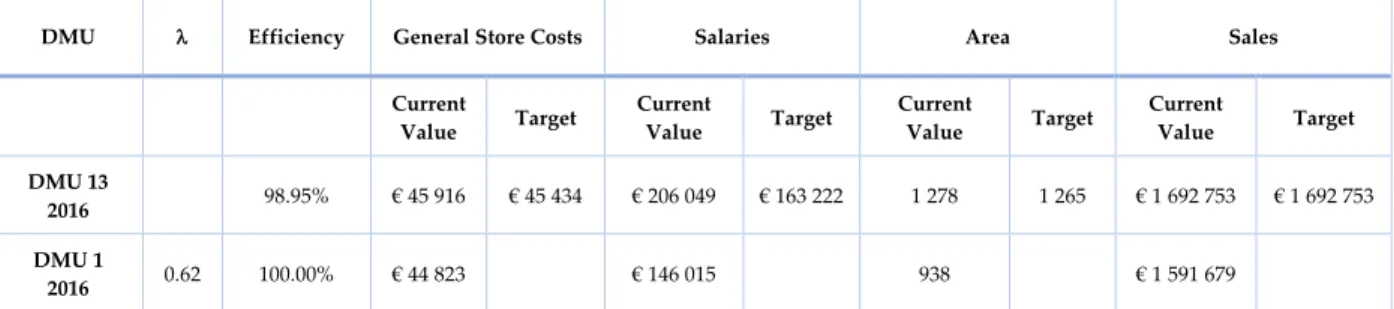
Table 11 - Efficiency, input and output values for store DMU 13 in 2016 and selected benchmark ... 68
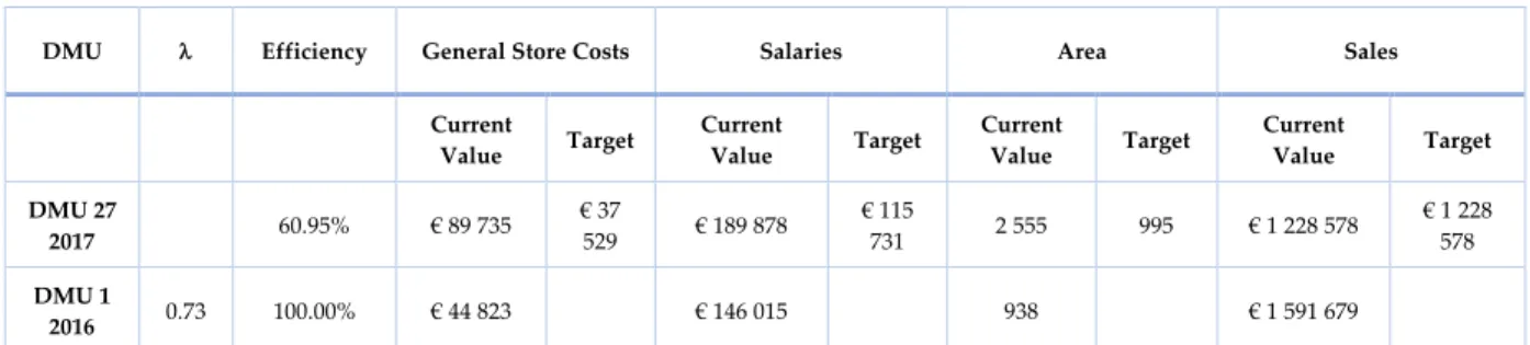
Table 12 - Efficiency, input and output values for store DMU 27 in 2017 and selected benchmark ... 69
Table 13 - Efficiency, input and output values for store DMU 14 in 2016 and selected benchmarks ... 69
Table 14 - Inputs and outputs average values for the highest and lowest performing units ... 71
Table 15 - Sales, EBITDA and EBITDA margin for the eleven top performance units ... 72
Table 16 - Sales, EBITDA and EBITDA margin for the eleven bottom performance units ... 72
Table 17 - Tobit regression model results (aggregate of all analysed stores) ... 76
Table 18 - Average values of the environmental variables for the top and bottom performing units ... 79
Table 19 - Framework of the use of Data Envelopment Analysis and Tobit Regression Model studies (built out of in the literature review) ... 90
Table 20 - Population within the trade area ... 91
Table 21 - Average distance traveled by clients to each DeBorla Store ... 92
Table 22 - Number of Gato Preto, Espaço Casa, Area and CASA stores within the trade area ... 93
Table 23 – Store distance matrix to the nearest competitor ... 94
Table 24 - CRS, VRS, Scale Efficiency and Sources of technical efficiency results for all observations ... 97
Table 25 – Efficiency of each of the 27 stores per year and store average efficiency ... 98
Table 26 - Benchmarks results from the DEA model with VRS, without environmental variables... 100
Table 27 - Performance improvement goals for General Store Costs ... 101
Table 28 - Performance improvement goals for Salaries ... 102
Table 29 - Performance improvement goals for Area ... 103
Table 30 - Performance improvement goals for Sales ... 104
Table 31 - Store potential gains for input and output variables ... 105
Table 32 – Store location characterization: District, Municipality and Region of Continental Portugal ... 106
Acronyms
DEA Data Envelopment Analysis CCR Charnes, Cooper and Rhodes BBC Banker, Charnes and Cooper VRS Variable Return to Scale CRS Constant Return to Scale DMU Decision Making Unit OLS Ordinary Least Squares TE Technical Efficiency PTE Pure Technical Efficiency SE Scale Efficiency
QGIS Geographic Information System
Chapter 1 - Introduction
Today’s economic conjuncture is uncertain and this leads to a volatile economic profile of families. The response of retail sector to market’s volatility is being very dynamic and in constant transformation, as to meet the households’ needs everywhere and in an efficient way (i.e. to create more value with fewer resources). Ever increasing competition is a reality that retailers know well and always take into consideration, because it is a major challenge to their profitability. In a saturate retail market, firms have more and more necessity of improving their performance.
In most cases, firms performance assessment is based on operational and financial indicators, composing their financial statements, and the main indicator used to measure performance is profit. However, this approach have a number of limitations (Fernandes, 2007): (1) The profit being the only indicator may biase performance evaluation, because many different factors influence firm’s economic activity, such as location, trade area, etc. Therefore, a store that faces a lot of competition may attain less profit comparatively to others, though, if the store is making better use of resources, may achieve a superior performance. (2) An operational or financial ratio has a clear and evident interpretation if it is related to only one resource and one outcome. To seek a more extensive analysis, various ratios should be applied simultaneously. Nevertheless, each ratio could lead to different and contradictory statements on the firm’s performance. (3) In order to obtain an unique performance measure, an aggregated ratio should be considered, in spite of the inherent subjectivity in the definition of the weights attributed to each indicator.
Another trend in measuring firm’s performance is the comparison between the initially proposed objectives (as set in the planning of a firm’s budget) and the results actually achieved. When doing this, account must be taken that those objectives are defined through a number of simplified hypotheses, which could lead
to a deviation from reality, thus being another approach featuring limitations (Fernandes, 2007).
In order to decrease the impact of such limitations and obtain a more accurate and unbiased performance evaluation, two widely used methodologies have been applied in this dissertation: Data Envelopment Analysis (DEA) and Tobit Regression Model1.
1. Research objectives
The thesis is on store performance evaluation and improvement in the retail sector. To achieve this goal, two methodologies have been applied in a real business case. DESFO, SA was the retail sector group under study.
Firstly, Data Envelopment Analysis was the selected tool to evaluate store efficiency. The results provide a score for that efficiency, which allow us to know how efficient the stores are. In order to make a correct and impartial analysis, each store is evaluated by a comparison to its peers. So, could identify which stores are fully efficient and which are not. DEA also provides improvement goals for the inefficient units, in order to drive them to become completely efficient. These so-called improvement goals are linked to the variables - inputs and outputs - that compose the DEA model.
Secondly, a study of the impact that certain variables have on store efficiency, as measured by the previous methodology, should be undertaken.
These variables are not the same that characterize the DEA model, because the aim is to study the effect of variables that the stores do not have under their control. With the help of Tobit Regression Model, a multiple regression model was estimated to provide information on the statistical significance of those variables and
1 The Data Envelopment Analysis and Tobit Regression Model will be addressed in more detail in the following chapters.
quantifying the impact on efficiency. This allowed us to know which variables should be considered by the firm in the future when opening a new store.
2. Structure
In the first chapter, the purpose and motivation of the thesis is presented, as well as the research objectives and the methodologies used to pursue them. In the second chapter, a brief description of the firm used as real business case is presented. In Chapter 3, the used methodologies are theoretically and mathematically described. Chapter 4 proceeds with a literature review of those techniques and their practical applications to retail. In Chapter 5, a contextualization of the stores and a rigorous description of the variables that compose the available dataset are made. Chapter 6 advances with the development of the DEA model applied to a group of selected stores and with the display of the respective results. In Chapter 7, the environmental variables that impact store efficiency are presented. Last but not least, Chapter 8 outlines the conclusions of the research study and provides contributions for future work.
Chapter 2 – The empirical setting
1. The firm - DESFO SGPS, S.A.
DESFO was founded 30 years ago, in 1984. The name of the company, is a combination of Desicor and Forcargo, which were the first two companies in the group. Initially, the firm was specialized in the production of furniture. Along the years it has diversified production to other products and broaden activities to retail and logistics.
Nowadays, DESFO holds four independent business units: (1) Industry, where manufacturing is driven by efficiency and quality; (2) Retail, focusing on services and products that meet costumer’s demand; (3) Logistics, diversifying services in the supply chain; (4) Investments, where the firm commits to new projects and partnerships.
Desfo has 100% Portuguese capital and owns eight different brands: DESICOR and ONESKIN for manufactured product lines, DeBorla and MEGA in retail, FORCARGO and TRANSNAUTICA in logistics, and DESFOINVEST and DEKOINVEST in investments. All the activities are located in Portugal, except those of DEKOINVEST in Romenia and those of MEGA in Angola.
The strategy adopted by the company may be seen as opportunistic, always trying to take advantage of the business opportunities that were appearing over time. Initially, DeBorla started out as a discount store business, with the price playing a decisive role in the competitiveness. With its 2013 Joint Venture, DeBorla has become a household store, focusing on interior design products. Price was no longer the critical factor, with design, market trends and quality being of major importance.
In 1998, DeBorla opened the first store, and with that DESFO began its activity in Retail. DeBorla currently has 34 stores in Portugal, of which five are located in Madeira and Açores. DeBorla currently offers seven product categories, where Kitchen represents 21% of sales, Interior Design 20%, Storage 11%, Textile 10%, Garden 8% and Bathroom 7%.
Chapter 3 – Methodologies
1. Data Envelopment Analysis (DEA)
According to the extensive literature, Data Envelopment Analysis, also called DEA, is a nonparametric, deterministic approach and also a quantitative and analytic tool, that may be used to measure the performance of firms in different types of studies.
It is used to measure performance of Decision Making Units (DMUs), that convert multiple inputs (resources that the firm has in its power) into multiple outputs (results produced by the firm) (Thanassoulis, 2001). Since it handles data inputs and data outputs, it is known as a “data oriented” approach, as stated by (Cooper et al., 2011) and (Cooper et al., 2004). The correct identification of input and output variables in each specific case is obviously crucial so, as a general rule, the inputs and outputs used in a DEA model are chosen according to the specific firm’s strategy and objectives with the advice of the relevant literature.
The acceptance and use of DEA has been rapidly increasing. Examples of applications may be found in performance evaluation in many industries, hospitals, universities, cities, courts, and other businesses, including also the performance assessment of countries, regions, etc. (Cooper et al., 2004). Many benchmarking studies use DEA, allowing sources of inefficiency in many profitable firms to be identified.
As emphasized by several authors, namely (Thomas et al., 1998), DEA focus on frontiers, in other words, it identifies the limit of outcome/output attained by each DMU given a set of resources/inputs, instead of portraying a major trend as in Ordinary Least Squares (OLS) method, which gives an average performance.
As reinforced by (Banker & Morey, 1986), the purpose of a DEA model is to determine an efficiency level to each unit in the reference set, based on a peer performance comparison. These peers, called benchmarks, are the best performing units that can be used as role models for comparison in the evaluation of the less efficient units (Thomas et al., 1998). The set of efficient DMUs form a so-called “efficient frontier”, allowing the determination of efficient target levels of the inputs and outputs for the less efficient units, called non-frontier units (those levels that would render the units efficient).
(Farrell, 1957) is considered a pioneer in this matter, as he proposes a way of measuring efficiency. Observing that there were many restrictions when combining multiple inputs in any measure of efficiency, he proposed an approach to overcome this problem, extending the concept of productivity to a more general concept of efficiency. This concept is based on the extended Pareto-Koopmans definition (Koopmans, 1951) and is also known as Technical Efficiency: a unit is technically efficient if none of its inputs or outputs could be reduced or improved without, simultaneously, increasing or deteriorating other inputs or outputs. Thus, through the efficiency measurement of a DMU relatively to others similar DMUs, the concept of Relative Efficiency emerges (Cooper et al., 2004). This was formalized by (Charnes et al., 1978) and not by (Farrell, 1957), despite the fact that the definition is in agreement with Farrell’s models. The concept of Technical Efficiency was distinguished by (Farrell, 1957) from other concepts of efficiency, like Scale Efficiency.
Extending Farrell’s work considering only one output, the DEA methodology was introduced, in its present form, by (Charnes et al., 1978), with multiples inputs and outputs being considered in the analysis. They described DEA as a mathematical programming approach that helps building production frontiers, using only efficient DMUs where the output is maximized.
(Thomas et al., 1998) highlights relevant points that should be taken into consideration in DEA models, which are supported by (Parsons, 1992), (Thurik,
1992) and (Kamakura et al., 1996). First of all, weights should be assigned, when considering multiples inputs and outputs, because they will reflect the relative importance of each variable. Secondly, environmental variables that have an impact on efficiency, such as the location of a retail store or trade area factors, should be considered in the DEA models (directly or indirectly). The third point is that, traditional ordinary least squares, used to establish the input/output relation, is not ideal because it is based on averages. DEA, in fact, is more accurate than typical regression analysis when identifying efficient and inefficient units, since it considers each unit separately and compares each unit only with the most similar efficient units. Furthermore, DEA is much more effective when motivating and rewarding managers, like store managers, in the use of practices that could be observed in a specific store and transferred to other stores. A distinction between inputs under the control of store managers and the ones that only headquarters managers may have under control should obviously be made. Last but not least, more than one outcome should be taken into account, because DMU assessment always regards multiple and, in some cases conflicting, performance measures.
1.1 Basic Formulations of the DEA Methodology
The DEA methodology formulated by (Charnes et al., 1978) generalizes the single-output to single-input classical ratio definition to multiple single-outputs and inputs.
Consider n DMUs (j=1,…,n), which are referred to an entity evaluated by their ability to convert inputs into outputs, where each of the DMUs consumes m inputs (xm) and guarantees s outputs (ys). DEA is formulated as a mathematical
programming problem and is that it does not need weights to be pre-assigned to the inputs and outputs. Those weights are optimized by solving the DEA model. The goal is to maximize the ratio between the weighted outputs and the weighted inputs,
which can be formulated as a fractional programming model to evaluate the efficiency of each DMU in turn, as shown below:
𝑚𝑎𝑥 ℎ0 (𝑢,𝑣) = ∑ 𝑢𝑟 𝑟𝑦𝑟0 ∑ 𝑣𝑖 𝑖𝑥𝑖0 St: ∑ 𝑢𝑟 𝑟𝑦𝑟𝑗 ∑ 𝑣𝑖 𝑖𝑥𝑖𝑗 ≤ 1, j = 1,…,n, 𝑢𝑟 ≥ , r = 1,...,s, 𝑣𝑖 ≥ , i = 1,...,m. Where,
• is a very small positive number,
• 𝑗 is the index number related to each of the n DMUs, • 0 is the index of the DMU under analysis,
• 𝑦𝑟𝑗 and 𝑥𝑖𝑗 are the observed outputs and inputs, respectively, of the 𝐷𝑀𝑈𝑗,
• 𝑢𝑟 and 𝑣𝑖 represents the assign weights to the output and input,
respectively.
With this model an efficiency measure for any DMU is obtained, where the ratio of the total weighted output to the total weighted input for all DMUs is maximized, as shown by the previous equation. This is subjected to the constraint that for the ratio above every DMU must be less than or equal to one, ensuring that no unit will have an efficiency score greater than one. Thus, the efficiency measure of any 𝐷𝑀𝑈𝑗,
expressed as ℎ𝑗∗, assumes a value between 0 and 1, obtained by the optimal solution
values of the outputs 𝑦𝑟𝑗∗ and inputs 𝑥𝑖𝑗∗. Therefore, an unit could attain the
maximum efficiency score of 1 and, if that is the case, is an efficient unit; on the other hand, if the unit attains an efficiency score less than 1, it is an inefficient unit. The efficient units will form the efficiency frontier, with the inefficiency of the remaining units being measured by the distance to that frontier. Furthermore, through a peers
comparison, information is obtained about feasible input’s reductions, maintaining the levels of outputs. The input’s savings and, on the other hand, the output’s increases without increasing the levels of inputs are two approaches for the improvement of inefficient DMUs. It is therefore possible to determine the input’s and output’s target values for the inefficient DMUs to become fully efficient.
1.2 CCR and BCC models
The DEA model uses two important approaches, both of them analysing the relative efficiency of a DMU. The first approach is the so-called CCR (Charnes, Cooper and Rhodes) model, also called Constant Return to Scale (CRS) model introduced by (Charnes et al., 1978). The second formulation is the BCC (Banker, Charnes and Cooper) model, also called Variable Return to Scale (VRS) model by (Banker et al., 1984).
The selection of any of these models depends on the size variability of the DMUs. In the CCR model the units present a similar size, meaning that maximum efficiency is always achievable irrespective of the size of the DMU. Under the VRS model, only units of similar size are compared as it is assumed that size matters. The choice for one or another approach depends on the empirical setting and whether each of the above assumptions is the most adequate.
Both models can follow two type of orientations leading to an input-oriented model or an output-oriented model. In the first case, the goal is to minimize the inputs keeping the outputs constant. In the latter case, the objective is to maximize the outputs keeping the inputs constant. The efficiency scores always fall in a range between 0 and 1, regardless if it is a CRS or a VRS model.
In brief, two aspects have to be considered in order to proceed with this method and to measure efficiency in an accurate way. Firstly, it is important to choose
the returns-to-scale is needed, a firms activity may be characterized as having Constant Return to Scale or Variable Return to Scale. In order to compare both approaches, the CCR and BCC models have to be calculated.
(Banker et al., 1984) developed a linear programming problem, in order to compute the efficiency scores as follows:
BCC model: Input Oriented2
𝑒𝑗0 = max 𝜃𝑗0 = ∑ 𝑢𝑟𝑦𝑟𝑗0+ 𝑢 𝑠 𝑟=1 St: ∑ 𝑢𝑟𝑦𝑟𝑗 𝑠 𝑟=1 − ∑ 𝑣𝑖𝑥𝑖𝑗 𝑚 𝑖=1 ≤ 0 ∑ 𝑣𝑖 𝑚 𝑖=1 𝑥𝑖0= 1 𝑢𝑟 ≥ 𝜀, 𝑟 = 1, … , 𝑠 𝑣𝑖 ≥ 𝜀, 𝑖 = 1, … , 𝑚 Where:
• 𝜀 is a very small positive number • 𝑢 is free
By using dual linear programming, the BCC model presented above can be developed as an “Envelopment Model”:
2 In this section, only the BCC model with an input orientation will be presented, because those models will be the ones used in this study.
𝑒𝑗0 = 𝑚𝑖𝑛 𝜃𝑗0 − 𝜀(∑ 𝑠𝑖−+ ∑ 𝑠𝑟+ 𝑠 𝑟=1 ) 𝑚 𝑖=1 St: ∑ 𝑥𝑖𝑗𝜆𝑗+ 𝑠𝑖− = 𝜃𝑥𝑖0, 𝑖 = 1, … , 𝑚, 𝑛 𝑗=1 ∑ 𝑦𝑟𝑗𝜆𝑗− 𝑠𝑟+ = 𝑦 𝑟0, 𝑟 = 1, … , 𝑠, 𝑛 𝑗=1 ∑ 𝜆𝑗 = 1 𝑛 𝑗=1 𝜆𝑗, 𝑠𝑖−, 𝑠𝑟+ ≥ 0, ∀𝑖 , 𝑗, 𝑟 Where: • 𝑠𝑖− and 𝑠
𝑟+ are the slack values of the inputs and outputs, respectively
• 𝜃𝑘(k=1,…,n) is the efficiency value of the DMUk
• 𝜀 is a very small positive number
This model identifies the peers of the DMU under analysis (𝐷𝑀𝑈𝑗0), allowing the
DMU relative efficiency (𝜃𝑗0) and optimal inputs and outputs values to be measured.
This optimal values are given by a linear combination (∑𝑛𝑗=1𝑥𝑖𝑗𝜆𝑗, ∑𝑛𝑗=1𝑦𝑟𝑗𝜆𝑗) of the
benchmarks of 𝐷𝑀𝑈𝑗0 – the efficient units that dominate the inputs and outputs of
𝐷𝑀𝑈𝑗0.
Taking into account the above mentioned definition of efficiency and applying it to these models, a DMU is completely efficient, if 𝜃∗ = 1 and 𝑠𝑖−∗= 𝑠𝑟+∗= 0.
However, a DMU is weakly efficient if at least one slack is different from zero, 𝑠𝑖−∗≠ 0 and/or 𝑠𝑟+∗≠ 0, for any i and r (Cook & Zhu, 2005).
The technical efficiency of the 𝐷𝑀𝑈𝑗0 is attained by reducing the inputs by the
value. On the other hand, the technical efficiency of 𝐷𝑀𝑈0 can be achieved by
increasing the outputs by the value permitted by the slack. In this case, the output target value is given by the product of the observed output with the efficiency score obtained, minus the slack value.
The values of the output and input targets are measured as following: 𝑥̂ = 𝜃𝑖0 ∗𝑥𝑖0− 𝑠𝑖−∗ 𝑖 = 1, … , 𝑚
𝑦̂ = 𝑦𝑟0 𝑟0+ 𝑠𝑟+∗ 𝑟 = 1, … , 𝑠
Through this model, information can be provided about the slacks of each input 𝑠𝑖−∗ and output 𝑠
𝑟+∗. As mentioned above, if a DMU has a slack that is not null, it
means that that unit is weakly efficient, and hence that value corresponds to the amount of input reduction and output increase feasible, so that unit becomes fully efficient.
Mathematically, the difference between the BCC model and the CRS model can be demonstrated as following: a constraint is withdrawn to the former model, ∑𝑛𝑗=1𝜆𝑗 =
1, which implicates the removal of the variable 𝑢 in the dual problems.
1.3 Scale effects
As previously mentioned, two approaches may be used to evaluate the performance of the DMUs: CRS and VRS.
The differences between a CRS frontier and a VRS frontier are shown in Figure 1. The CRS frontier is represented by a straight line, where 𝐷𝑀𝑈𝐸 is the only efficient
unit belonging to it. However, in the case of the VRS frontier, a convexity constraint is added to the model, ∑𝑛𝑗=1𝜆𝑗 = 1, which leads to the frontier being piece-wise linear
Figure 1 – CRS and VRS frontiers according to (Banker et al., 1984)
When looking at the VRS frontier, DMUs B and C produce their outputs with a different scale, comparatively to DMU E. More concretely, DMU B shows increasing returns to scale, because an increase of an input leads to a proportionally larger increase in the output; unlike, DMU C shows decreasing returns to scale, for the fact that an increase of an input leads to a proportionally smaller increase in the output. So, with the CRS model we estimate a technical and also a scale efficiency, opposing to the VRS model that does not include the scale efficiency. It comes out from Figure 1 that:
CRS efficiency ratio = Technical Efficiency (TE) of DMU A = 𝑀𝑁𝑀𝐴.
VRS efficiency ratio = Pure Technical Efficiency (PTE) of DMU A= 𝑀𝐵𝑀𝐴.
Scale Efficiency represents the impact of the scale of the operation of a DMU, and is measured by the ratio between the CRS efficiency ratio and the VRS efficiency ratio, 𝑃𝑇𝐸𝑇𝐸.
Scale Efficiency (SE) ratio of DMU A = 𝑉𝑅𝑆𝐶𝑅𝑆 = 𝑀𝑁𝑀𝐵.
According to the expressions above, the sources of technical inefficiency of a DMU can be the result of: an inefficient operation (PTE), an unproductive scale (SE), or both (PTE and SE).
To understand what type of returns to scale characterize the efficient frontier, we can compute scale effects. If the DMU shows evidence of scale effects, then the wise choice is to proceed with VRS, otherwise CRS should be pursued (Dyson et al., 2001).
2. Tobit Regression Model
In order to analyse the drivers that impact the performance of a firm, the most common model used is a regression model. However, as stated by (Ko et al., 2017), a general regression model as the Ordinary Least Squares (OLS), is not able to analyse the factors that impact efficiency measured by DEA. In fact, with the efficiency value limited to a range between 0 and 1 the OLS could lead to biased estimates or invalid inferences. This is corroborated by the fact that the values estimated by OLS regression models could assume values inferior to 0 or superior to 1, thus out of the limited range that characterize the efficiency scores [0, 1]. Tobit Regression Model (Tobin, 1958) can overcome the above limitation, since it accounts for the possibility of truncated dependent variables.
(Coelli et al., 2005) proposed the identification of the factors that impact and are determinant to the DMUs efficiency, using a two stage approach. In a first step, the efficiency scores of the DMUs are obtained through a DEA model and, in a second step, the most impactful variables in those scores are found by using a Tobit Regression Model. Here, the dependent variable is characterized by the efficiency scores and the independent variables are the ones that could influence the dependent variable.
Many studies point out that the variables used in the DEA model are inherently dependent on the efficiency scores. Hence, the estimates developed in this second-stage will be biased and inconsistent (Yu & Ramanathan, 2008). In order to overcome this problem, authors like (Simar & Wilson, 2007) and (Coelli et al., 2005) suggest the application of a bootstrapping technique allowing best practices to improve performance.
As stated earlier, this model is useful when the dependent variable of this model is restricted to a certain range of values. The model is represented as:
𝑦𝑖∗ = 𝛽 0+ 𝛽1𝑥1𝑖+ 𝛽2𝑥2𝑖+ ⋯ + 𝑢𝑖 𝑖𝑓 𝑦𝑖∗ ≤ 0, 𝑡ℎ𝑒𝑛 𝑦 𝑖 = 0 𝑖𝑓 𝑦𝑖∗ ≥ 1, 𝑡ℎ𝑒𝑛 𝑦 𝑖 = 1 𝑖𝑓 0 < 𝑦𝑖∗< 1, 𝑡ℎ𝑒𝑛 𝑦 𝑖 = 𝑦𝑖∗ Where:
• 𝑦𝑖 is the efficiency score of the 𝐷𝑀𝑈𝑖that is calculated by DEA,
• 𝑥1𝑖 , 𝑥2𝑖 , … are the values of independent variables of the 𝐷𝑀𝑈𝑖,
• 𝛽1, 𝛽2, …. are the coefficients of the independent variables, which will
determine the expected effect of the independent variables on efficiency.
This method is very important to identify the drivers that have influence on the efficiency score (𝑦𝑖), that it is our dependent variable, and their impact. The results of
this model provide information about two important parameters. The p-value and the 𝑅2, as it will be shown in practice in Chapter 7. The p-value of the independent variables represents their statistical significance: if a variable is statistically significant (p-value < level of significance), means that the variable has impact on efficiency. The 𝑹𝟐 represents the percentage of the efficiency variability caused by the model, more concretely, through the independent variables that compose the regression model.
Chapter 4 - Literature Review
1. Studies on retail performance
DEA has been used in many application domains, one of which is retail. In this chapter, the methodologies used to analyse retail performance will be reviewed.
(Almohri et al., 2018) identify the drivers that impact the performance of an automotive dealership in comparison with similar dealerships and propose to rely on optimization techniques as to offer dealerships tailored recommendations. To achieve such objective, three techniques were applied. First, a clustering technique with filtered data from internal and external sources was used in order to obtain a group of similar stores where performance evaluation could be estimated more accurately.Second, an effective Finite Mixture of Regressions technique was used to undertake model-based clustering and to model store performance. This technique was based on competitive learning and clustering stores into a number of homogeneous groups, allowing effective performance modelling and the identification of practices to be used as benchmarks for less efficient stores. Finally, an optimization model was used to tailor recommendations for individual stores in the clusters, as to enable simultaneous improvement of store profitability and sales.
(Vyt & Cliquet, 2017) use many approaches to develop store performance standards, in order to fairly distribute rewards for managers as a function of the performances they achieve. First, they rank the stores in two ways: a store ranking by retailers and by using a two-step DEA method; second, they determine the so-called store’s profile. In a first step, the retailers are clustered along the retail chain using two criteria: location (stores are classified as belonging to a rural or a urban area) and sales area (stores are classified as having more or less than 1500m2). Then,
cluster. As to allow for comparative analysis, efficiencies for every store and for each cluster have been estimated. Finally, a two-step DEA model was used: initially, a DEA model assessed the individual efficiency of stores; then an Ordinary Least Squares (OLS) regression was used to know which variables impact on efficiency scores.
Likewise this last study, many authors adopt a two-stage procedure to evaluate performance. (Barros, 2006), (Vyt, 2008) and (Xavier et al., 2015), measured retailers efficiency in Portuguese hypermarkets and supermarkets, in a French supermarket retail chain and in a Portuguese fast fashion retailing sector, respectively. All have adopted a DEA model to evaluate the relative efficiency of each store and regression models to find out which variables impact on the efficiency score extracted by the previous stage. However, the first authorused a Tobit Regression Model, the second author used OLS regression, and the third used a quantile regression technique. One should note that they have all used a bootstrap technique, because the efficient scores are correlated to the explanatory variables of the regression model, in order to avoid biased and inconsistent results.
In (Gandhi & Shankar, 2016), the authors wanted to know the current level of performance of Indian retailers and to find out how they could plan and improve their operations and profitability in terms of the company, the store, the merchandise category, or even ate the sku (Stock Keeping Unit) level. For such purpose, they have used two methods: Strategic Resource Management (SRM) and DEA. First, two generic Indian retailers (Shoppers Stop and Trent) were compared using the SRM model, and then they have been benchmarked with a greater retailer (Walmart). In order to validate these results, a DEA model has been used to assess the efficiency of 11 retailers, including the two considered in the previous analysis.
(Yu & Ramanathan, 2008) and later (Yu & Ramanathan, 2009) studied the performance of firms in the retail sector. The first study has been undertaken in the UK and deals with different types of business, like food retailing, home appliances retailing and department store retailing; the second case has targeted retailers in
China. In both cases, the same three methodologies have been used: Data Envelopment Analysis (DEA), with the objective of measuring the technical and scale efficiency of the retailers, Malmquist productivity index (MPI), analysing changes in the patterns of efficiency during the period in question, and a bootstrapped Tobit Regression Model, that has the power to calculate the impact of environmental variables on the efficiency levels measured by the DEA model. The studies reached the conclusions that only ten out of 41 UK retailers are technically efficient and only seven out of 61 Chinese retailers are technically efficient; another conclusion was that 50% of the UK retail firms and 37.3% of the Chinese retail firms have registered progress in terms of MPI during the period under analysis; and finally, that three out of five environmental factors have significant influence in the UK retail efficiency while among the Chinese retail firms only one out of five environmental factors has that impact.
2. DEA applied to the benchmark of retail stores
Benchmarking is a powerful method to study competition between firms in the retail sector, with DEA being instrumental to analyse the efficiency of comparable firms (Yu & Ramanathan, 2008).
This section will review a set of studies that have used this method, identifying which type of data and which models were used to fulfil the objective of assessing the relative efficiency of a store.
(Barros & Alves, 2003) and (Barros, 2006) studied the efficiency of Portuguese supermarkets and hypermarkets. In the first case, 47 retail stores were analysed using a cross-section data for the year 2000; the second study targets 22 retail stores using panel data between 1998 and 2003, with 132 observations being considered. Both studies consider an output-oriented model, with a Variable Return-to-Scale
central management. For comparative terms, a Constant Return-to Scale (CRS) hypothesis was used and the ratio between these efficiency scores, measured by VRS and CRS, has provided the Scale Efficiency measure. The results have shown that scale economies are a dominant source of inefficiency.
(Vyt, 2008) measured the relative efficiency of 38 stores of a French supermarket retail chain. In this case, three DEA models were used. In all models, an output-oriented model under VRS was used. In the first model, the exogenous variables were considered as fixed. In the second model, all inputs were allowed to vary. The third model, consisted on a two-step approach, with the first step using DEA using with store variables only, and the second step an Ordinary Least Square (OLS) regression. The results have shown that the first two models have poor discriminant power, because all the stores were classified as efficient, regardless of the fact that, in the second model, one store was considered as inefficient. With the third model, only 15 supermarkets were assessed as efficient.
(Perrigot & Barros, 2008) have also assessed the technical efficiency of French retailers. In this study, data from 11 stores with a panel data between 2000 and 2004 grouping 55 observations has been used. A output-oriented model with a VRS hypothesis was considered with the objective of maximizing their production. They have also used a CRS hypothesis and the conclusion was that both hypotheses lead to high average efficiency scores, which means that the dominant source of efficiency is scale, contrary to the conclusions of the previous studies. Apart from these two models, two more have been considered: cross-efficiency and super-efficiency DEA models, allowing to discriminate between the super-efficiency units given by CRS and VRS models.
Measuring stores performance is not only about assessing supermarket and hypermarket stores, but it can be done with other retail industries. For example, (Xavier et al., 2015) have used data from 40 clothing stores, both from winter and summer collections, between 2010 and 2013. An input-oriented model was chosen, because of the fact that retailers had relatively less control on the outputs. Both CRS
and VRS models were considered and the results have shown that there were not problems of scale, because scale efficiency was higher than pure technical efficiency.
(Lau, 2013) has targeted a major Australian retailer, assessing six stores in the retailer’s network in the year 2009. An input oriented model was used, with both VRS and CRS hypotheses to compare store performance. The results show that in both hypotheses the same efficient store is elected, and that low efficiency scores are due mainly to scale inefficiency. A slack analysis is also undertaken with the purpose of measuring the target input and output values of the stores.
(Thomas et al., 1998) measure the performance of 500 domestic outlets selling “moderately priced home furnishings and household items”. Two procedures have been used to measure the performance of those stores. Initially, an output-oriented model was used with two outputs and 16 inputs, discriminating the inputs that store managers have under control from those they do not control at all. The conclusion was that seven of the stores are fully efficient, being positioned on the efficient frontier. Additionally, the authors wanted to identify the critical success factors (CSF) and, for such matter, they proceeded with a multivariate analysis of variance (MANOVA). For that purpose, the inputs were measured based on the efficiency level determined by the DEA model and subsequently divided into quartiles using that criteria. Then, the differences between the outputs in all of the quartiles were evaluated. The results of this test showed that there were differences in both outputs across the quartiles (F = 80.41, > 0.001). In brief, the results of the MANOVA suggested that there were specific factors associated with high store efficiency.
As stated previously (Yu & Ramanathan, 2008) and later (Yu & Ramanathan, 2009), used DEA to evaluate the performance of 41 UK and 61 Chinese retailers, respectively, both using a panel data. They chose to calculate VRS, CRS and Scale efficiencies separately, using an output-oriented model. The results point out that in both approaches, the firms that are found to be fully efficient with the CRS model, are also completely efficient with the VRS model, which means that those retailers
efficient firms is higher. This means that these firms generate the maximum outputs for a given set of inputs, unlike the inefficient ones that were not able to do it.
2.1 Factors that influence performance
The variables selected as inputs and outputs, when applying DEA, and the explanatory variables considered in the Tobit Regression Model are of utmost importance. In both methods, variable selection should reflect the firm’s goals, objectives, key performance indicators (KPIs) and sales, and also take into consideration the variables used in previous studies.
According to the literature, the more commonly used variables as outputs are: “Sales” ((Vyt, 2008); (Vyt & Cliquet, 2017); ((Barros, 2006); (Yu & Ramanathan, 2008); (Yu & Ramanathan, 2009); (Xavier et al., 2015); (Gandhi & Shankar, 2016); (Uyar et al., 2013); (Barros & Alves, 2003); (Yu & Ramanathan, 2009); (Ko et al., 2017); (Gandhi & Shankar, 2014); (Moreno & Sanz-Triguero, 2011); (Donthu & Yoo, 1998); (Perrigot & Barros, 2008); (Thomas et al., 1998)), “EBITDA” ((Barros, 2006); (Yu & Ramanathan, 2008); (Yu & Ramanathan, 2009); (Xavier et al., 2015); (Uyar et al., 2013); (Barros & Alves, 2003); (Moreno & Sanz-Triguero, 2011)), and “Profit” ((Uyar et al., 2013); (Gandhi & Shankar, 2014); (Perrigot & Barros, 2008); (Thomas et al., 1998)).
When choosing which inputs should be applied, the literature distinguishes controllable (also known as discretionary) from uncontrollable (also known as non-discretionary) variables. Controllable inputs are those that each of the DMUs has under control, unlike the uncontrollable inputs, which are dependent on central management or other external actors. Thus, the authors end up choosing the first ones, because it is through them that DMUs can gain competitive advantage: “Number of employees” ((Barros, 2006); (Yu & Ramanathan, 2008); (Yu & Ramanathan, 2009); (Gandhi & Shankar, 2016); (Uyar et al., 2013); (Barros & Alves,
2003); (Ko et al., 2017); (Perrigot & Barros, 2008); (Vyt, 2008); (Vyt & Cliquet, 2017); (Thomas et al., 1998); (Moreno & Sanz-Triguero, 2011); (Thomas et al., 1998)), “Sales area” ((Yu & Ramanathan, 2009); (Gandhi & Shankar, 2016); (Uyar et al., 2013); (Pestana Barros & Alves, 2003); (Ko et al., 2017); (Vyt, 2008); (Vyt & Cliquet, 2017); (Ko et al., 2017); (Donthu & Yoo, 1998)), “Number of stores” ((Barros, 2006); (Gandhi & Shankar, 2014)), “Assets” ((Barros, 2006); (Yu & Ramanathan, 2008); (Xavier et al., 2015); (Perrigot & Barros, 2008); (Gandhi & Shankar, 2014); (Moreno & Sanz-Triguero, 2011)), “Salaries” ((Xavier et al., 2015); (Uyar et al., 2013); (Barros & Alves, 2003); (Gandhi & Shankar, 2014); (Thomas et al., 1998); (Moreno & Sanz-Triguero, 2011); (Thomas et al., 1998)), “Rental cost” ((Xavier et al., 2015); (Ko et al., 2017); (Vyt, 2008); (Vyt & Cliquet, 2017); (Thomas et al., 1998)), and “Inventory” ((Gandhi & Shankar, 2016); (Uyar et al., 2013); (Thomas et al., 1998); (Moreno & Sanz-Triguero, 2011) (Barros & Alves, 2003)).
Although many authors put aside the uncontrollable inputs (also known as environmental variables), some authors consider them, since they may strongly affect the stores’ performance. Examples of those variables are: “Location” ((Barros, 2006); (Yu & Ramanathan, 2008); (Yu & Ramanathan, 2009); (Donthu & Yoo, 1998)), “Retail characteristics” ((Yu & Ramanathan, 2008); (Yu & Ramanathan, 2009)), “Competitors within the trade area” ((Ko et al., 2017); (Vyt, 2008); (Vyt & Cliquet, 2017)), “Ownership” ((Barros, 2006); (Yu & Ramanathan, 2008); (Yu & Ramanathan, 2009); (Gandhi & Shankar, 2014)), “Store age” ((Uyar et al., 2013); (Gandhi & Shankar, 2014); (Ko et al., 2017); (Barros & Alves, 2003); (Thomas et al., 1998); (Yu & Ramanathan, 2008); (Yu & Ramanathan, 2009); (Thomas et al., 1998)), “Population within the trade area” ((Ko et al., 2017); (Vyt, 2008); (Vyt & Cliquet, 2017); (Thomas et al., 1998); (Uyar et al., 2013)), and “Potential Market” ((Vyt, 2008); (Vyt & Cliquet, 2017)).
Chapter 5 – Description of the store set and dataset
The aim of this chapter is to present and characterize the stores targeted in this study, and also to describe the variables in the dataset. This step of the work is very important since we needed to capture in detail the reality of the DeBorla retail stores that were the subject of the project. The period of analysis is from January 2015 to December 2017.
1. Contextualization and description of the stores in the
dataset
From a total of 34 DeBorla stores, only 27 were considered in the dataset. The exclusion of seven stores was based in two criteria – location and time – since five of the stores are not located in Continental Portugal, and the other two only opened after the end of the period of analysis.
All stores in the sample are in what can be called a similar location, in the suburbs of urban centres. The 27 stores present an average sales area of 1645.1 𝑚2, ranging from the smallest one with 823.8 𝑚2 to the largest with 2946.8 𝑚2.
During the period of analysis, the stores remained unchanged in what regards the majority of their structural characteristics, like Retail, Store Visibility, Parking Space and Area.
2. Variables that compose the dataset
The dataset used is built by 18 variables, organized into six categories, classified as shown in Table 1:
Geography Demography Competition Structure Management Results
District Population within trade area
Number of “Gato Preto”
stores within trade area Age
General Store
Costs Sales Municipality Number of “Area” stores
within trade area Area Salaries EBITDA Number of “Espaço
Casa” stores within trade area
Store
Visibility Rent Number of “CASA”
stores within trade area
Parking Space Distance to nearest
competitor Retail
Table 1 - Categorization of variables of the dataset
Following to the categorization of the variables, it is important to make a detailed description of each of them, which is presented in Table 2. This table portrays the meaning of each variable, the type (discrete numeric variable, continuous numeric variable, nominal categorical variable, ordinal categorical variable), the units of measurement and finally some “Notes”, whenever an additional explanation is found helpful.
Variable Description Type Unit Notes
Population
within trade area Number of residents in a radius of x km
Numeric - Discrete Millions of people [1]
Retail 1 – the store is located in a retail space; 0 – stand alone
store
Categorical -
Nominal Number
Age Store age (last period of analysis 31-12-2017) Numeric -
Continuous Years
Sales Total value of store sales, in the period January 2015 –
December 2017
Numeric -
Continuous Euros
General store costs
Total value of store general costs, in the period January 2015 – December 2017
Numeric -
Continuous Euros
Salaries Total value of store personnel costs, in the period January
2015 – December 2017
Numeric -
Continuous Euros
Area Average sales area, in the period January 2015 – December
2017
Numeric - Continuous 𝑚
2
EBITDA Total value of store EBITDA, in the period January 2015 –
December 2017
Numeric -
Continuous Euros
Rent Total value of store rent, , in the period January 2015 –
December 2017 Numeric - Continuous Euros Number of “Gato Preto” stores within trade area
Number of Gato Preto stores in a radius of x km Numeric -
Discrete Number [2]
Number of “Area” stores within trade area
Number of Area stores in a radius of x km Numeric -
Discrete Number [2]
Number of “Espaço Casa”
stores within trade area
Number of Espaço Casa stores in a radius of x km Numeric -
Discrete Number [2]
Number of “CASA” stores within trade area
Number of CASA stores in a radius of x km Numeric -
Discrete Number [2]
Store Visibility
Indicates if the store has visibility, assuming the following values: 2) when the store is near a main road (having significant traffic during the week) and DeBorla brand is clearly identified by who is passing near the store; 1) if one
of the previous conditions is satisfied; 0) if none of the above conditions is verified.
Categorical -
Ordinal Number
Parking Space
Indicates if the store has parking space, assuming the following values: 0) when the store has no private parking
but there is parking nearby; 1) when the store has its own park, but there may be parking difficulties; 2) when the
store has a private parking.
Categorical -
Ordinal Number
District Name of the district where the store is located Categorical -
Nominal n.a
Municipality Name of the municipality where the store is located Categorical -
Nominal n.a
Distance to the nearest competitor
Distance of each DeBorla store to the closest competitor Numeric -
Continuous km [3]
From the Table above, the dataset is composed by 13 numerical variables (five discrete and eight continuous), and by five categorical variables (two ordinal and three nominal).
Assuming that most of the variables are clearly defined in Table 2, further analysis is now presented in the cases signalled in the Notes column.
[1] In order to determine the “population within trade area”, an open-source Geographic Information System (QGIS) software was used. The following steps were followed:
1. The coordinates (latitude, longitude) of each DeBorla store where inserted (Figure 2);
2. A “buffer” was created for each DeBorla store, as a surrounding area with a radius of 34 km (Figure 2), setting a demarcated area of influence;
3. The number of total residents3 within the “buffer” around of each DeBorla
store (see Figure 3, Table 20 in Appendix B.1), was estimated.
Figure 2 - Locations and respective surrounding areas for each DeBorla store
3 Number of total residents: this information was provided by Census 2011, the last with the available compatible format data for QGIS.
Figure 3 - Population within the trade area
The radius of 34 km of the “buffers” was derived from an estimate on how far DeBorla customers are willing to drive in order to reach each store. To answer this question the QGIS software was used, to estimate the surrounding area, in a process encompassing three different steps:
1. The coordinates (latitude, longitude) of the address of each DeBorla customer were inserted in the software, this information being provided by the firm (Figure 4);
2. The distance between the address of each customer and the location of DeBorla stores was measured. In order to allow that, the firm provided information on the stores that each customer goes to. The distance traveled by each customer to the respective store could then be calculated;
3. The average distance travelled by the customers to each DeBorla store was finally calculated (see Table 22 in Appendix B.2)4.
Figure 4 - Locations of DeBorla stores and their customers
As shown by Table 21, three of the stores (DMU 1, DMU 13 and DMU 24) are outliers, because of the unusually large average distances travelled by their customers. All these stores are located in Algarve, south of Portugal, and the explanation for being outliers is that their customers take the advantage of the fact that they are on vacation to buy in those DeBorla stores. For that reason, these outliers will not be taken into consideration into the determination of the average distance travelled by customers. As we can see in Table 3, the average travelled distance for all DeBorla stores, excluding the outliers (DMU 1, DMU 13 and DMU 24), is quite similar to the median travelled distance for all stores, including the outliers.
Average distance (excluding DMU 1, DMU 13, DMU 24) 41 km
Median distance (all stores) 34 km
So, the radius of the buffers was calculated using the median of the distances travelled by the customers to access the stores.
[3] To determine the “number of each of the competitors within trade area”, the QGIS software was used, going through the following steps:
1. The coordinates (latitude, longitude) of all stores, DeBorla and different competitors were inserted (Figure 5);
2. The number of each of the competitors within each buffer of each DeBorla store was calculated (Table 22, Appendix B.3).
Figure 5 - Location of DeBorla stores (red) and competitors stores (green)
[4] To determine the “distance to the nearest competitor”, the QGIS software was used, by:
1. Inserting the coordinates (latitude, longitude) of all stores, DeBorla and competitors (Figure 5);
Chapter 6 - Store Performance Evaluation
The aim of this chapter is to assess store performance in DeBorla group, by determining their efficiency scores through a DEA model, as well as to set improvement goals to the stores5. The model is expected to be able to evaluate the
capacity of the stores to generate output based on the existing inputs that contribute the most to the profitability of the stores.
In the present analysis, 27 stores are considered with panel data of three consecutive years, with a total of 81 observations. In fact, only 71 observations are being analysed, because some of the DMUs were not operating along all those years, namely the stores that opened in 2015 and 2016.
Regarding the DEA model used, both Constant Return to Scale (CRS) and Variable Return to Scale (VRS) models have been considered, in order to analyse different types of efficiency: technical efficiency (TE), pure technical efficiency (PTE) and scale efficiency (SE). Further than that, it was considered of major relevance to know which returns to scale characterize each of the stores, as well as to identify the existence of scale effects by using a non-parametric test. An input-oriented DEA model was used, because store managers have clearly more control on their inputs than on their outputs.
1. Selection of variables
The selection of the variables is a very important step in the development of the DEA model. This was done, taking into consideration an extensive literature review6
and also the objectives that were set by the firm.
In this process we first considered only discretionary variables, those that the store management can have some control upon, and excluded contextual variables related to the market and the competition.
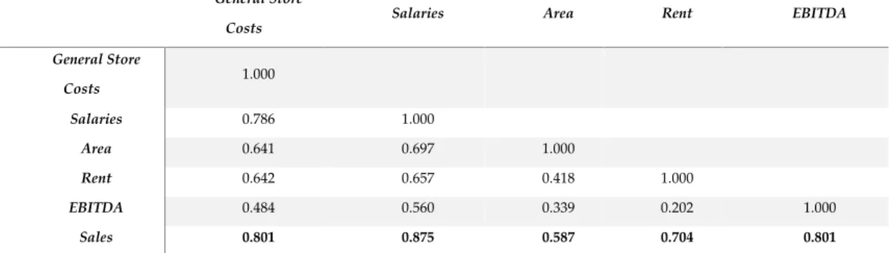
Table 4 shows a correlation matrix7 between the discretionary variables chosen to
be included in the model. Through this matrix we are able to infer that there is a strong positive correlation between the variables selected as inputs (General Store Costs, Salaries, Area and Rent) and the variables selected as outputs (Sales and EBITDA). This means that these output variables depend positively on the input variables contributing to their growth. However, both outputs have a strong correlation, which makes sense because Sales is a very important variable that contributes positively to EBITDA. We have therefore decided to opt for only one of these variables, and Sales was chosen because it is the output exhibiting the strongest relation with the other variables. A decision was also made of not including Rent in the model, even though it shows a strong correlation with the output Sales. This is because some of the stores belong to the company and do not pay a Rent and if this variable were to be included in the model it would distort the results.
6 Chapter 4 and Appendix A, put forward evidence that the variables used in the present study are fully corroborated by the literature.
7 The correlation matrix was constructed using software R, a free software package for statistical computing, specifically the Pearson Correlation analysis that studies the correlation or linear dependence between two variables. The results belong to an interval between -1 and 1 (-1 means that the variables have a perfect negative correlation; 0 means that the variables do not depend linearly from to one another; 1 means that the variables have a perfect positive correlation).


![Figure 6 – Store efficiency distribution with VRS Mean [all stores] Mean [inefficient stores] Median](https://thumb-eu.123doks.com/thumbv2/123dok_br/14948734.1003243/60.892.214.690.143.408/figure-store-efficiency-distribution-stores-inefficient-stores-median.webp)