Improvement of algorithms for the assessment of air quality and atmospheric composition from observations of spectral radiances

(1)

INSTITUTO DE INVESTIGAÇÃO E FORMAÇÃO AVANÇADA ÉVORA, ABRIL 2015

ORIENTADOR: DoutorDaniele Bortoli

CO- ORIENTADORA: Professora Doutora Ana Maria Almeida e Silva

Tese apresentada à Universidade de Évora

para obtenção do Grau de Doutor em Ciências da Terra e do Espaço.

Especialidade: Física da Atmosfera e do Clima.

Ana Filipa Alves Real Domingues

IMPROVEMENT OF ALGORITMS FOR

THE ASSESSMENT OF AIR QUALITY

AND ATMOSPHERIC COMPOSITION

FROM OBSERVATION OF SPECTRAL

RADIANCES

(2)

(3)

ÉVORA, ABRIL 2015

ORIENTADOR: DoutorDaniele Bortoli

CO- ORIENTADORA: Professora Doutora Ana Maria Almeida e Silva

Tese apresentada à Universidade de Évora

para obtenção do Grau de Doutor em Ciências da Terra e do Espaço

Especialidade: Física da Atmosfera e do Clima

Ana Filipa Alves Real Domingues

IMPROVEMENT OF ALGORITMS FOR

THE ASSESSMENT OF AIR QUALITY

AND ATMOSPHERIC COMPOSITION

FROM OBSERVATION OF SPECTRAL

RADIANCES

(4)

(5)

Acknowledgments

I am sincerely grateful to my supervisors Dr. Daniele Bortoli and Profª Dr. Ana Maria Silva for their guidance, availability, generosity and friendship through the development of this work. They have accompanied me in every step of this journey and inspired me to move forward. I am also thankful to Geophysics Centre of Évora and University of Évora for providing all the resources needed for the development of this work. And also for providing the means to extend my education through the participation in complementary courses and workshops and in national and international conferences.

I want to acknowledge to my CGE colleagues (Dr. Dina Santos, Vanda Salgueiro, Marta Melgão, Dr. Sérgio Pereira, Dr. Miguel Potes, Flávio Couto, Profª Dr. Maria João Costa, Prof. Dr. Rui Salgado, Dr. Manuel Antón, Dr. Pavan Kulkarni) for the good atmosphere at the office. I am thankful in particular to Profª Dr. Maria João Costa for her support and encouragement, to Dr. Manuel Antón for his availability in sharing his knowledge, and to Vanda Salgueiro for her valuable tips in MATLAB.

I also have to acknowledge to Lyzia Bensehil from Laboratoire de Météorologie et Dynamique (LMD), to Dr. Frederick Tack and Dr. Nicolas Theys from Belgian Institute for Space Aeronomy (BIRA-IASB), to Professor Alain Sarkissian and Dr. Florence Goutail from Laboratoire from LATMOS, to Dr. G.S. Meena from the Indian Institute of Tropical Meteorology, to Dr. Andreas Richter and Dr. Alexei Rosanov from Institute of Environmental Physics- University of Bremen (IUP Bremen) and Dr. Janis Pukite from Max Plack INstitute from MAinz (MPI), for articles, data and clarifications. I would like to thanks also Dr. Margherita Premuda, Dr. Samuele Masieri and Dr. Giorgio Giovanelli, researchers of the Institute for Atmospheric Science and Climate/ National Council for the Research (ISAC/CNR) in Bologna-Italy, for their advice in the use of the radiative transfer models.

Fundação para a Ciência e a Tecnologia (FCT) funded this work with the grant FCT- SFRH/BD/44920/2008. This grant was also valuable because supported partially my participation in conferences which were important for the diffusion and improvement of this research. This work was financed through other projects as well like the FEDER (Programa Operacional Factores de Competitividade – COMPETE) and national funding through FCT in the framework of project FCOMP-01-0124-FEDER-014024 (Refª. FCT PTDC/AAC-CLI/114031/2009), PTDC/CTE-ATM/65307/2006, PROPOLAR SPATRAM-MIGE and POCI/AMB/59774/2004.

(6)

I also acknowledge for the financial support provided by the French program LABEX that allowed for my participation in the European Research Course on Atmospheres organized by Université Joseph Fourier & CNRS which was a valuable educational experience for the conclusion of this thesis.

I gratefully acknowledge also to scientists that participate in the acquirement and provision of the environmental data and the following institutions:

• NOAA Air Resources Laboratory for the provision of the HYSPLIT data.

• ESA team for the accomplishment of all satellite missions and NO2 and O3 total columns

data

• SCIAMACHY team and in particular to Dr. Andreas Richter for his availability in the explanation of SCHIAMACHY products

• OMI team for the accomplishment of all satellite missions and for NO2, O3 and BrO total

columns data

• GOME-2 team for the accomplishment of all satellite missions and for NO2 and BrO total

columns data

• GOME team for the accomplishment of all satellite missions and for O3 total columns

data

• IUP Bremen team lead by Prof. J.P. Burrows for providing the data sets of NO2 vertical profiles by Dr. Alexei Rosanov

• BIRA- IASB UV-Visible DOAS group for BrO total columns from GOME-2 data by Dr. Nicolas Theys

• MPI, Mainz team for the SCIAMACHY NO2 vertical profiles by Dr. Janis Pukite

And last (but not the least) my sincere gratitude for the support of my friends Rute Feiteira, João Marques, Raquel Pina, José Garcez, Sofia Pinto, Filomena Mascarenhas and family. My deepest regards to my father Joaquim Domingues, husband Luís Bengala, daughter Joana Bengala and to my dearest mother Digna Domingues for their infinite love, care and patient.

(7)

i

List of Figures

Figure 2.1 - Typical vertical distribution of the concentration of chemical atmospheric

constituents under about 120 km (from Liou, 2002.) ... 9 Figure 2.2- Temperature variation in Earth’s atmosphere (from Platt & Stutz, 2008). ... 9 Figure 2.3- Variation of atmospheric pressure in Earth’s atmosphere with altitude in the

Earth’s atmosphere for tropical regions, mid latitudes in summer and winter, and high latitude sub arctic summer and winter (from Burrows et al., 2011). ... 11 Figure 2.4- Spatial and temporal scales variability of some atmospheric gases (from Platt &

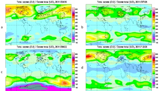
Stutz, 2008). ... 12 Figure 2.5 - Global distribution of Total Ozone (DU) varying with latitude and time of the year

(from http://exp-studies.tor.ec.gc.ca/e/ozone/Curr_map.htm). ... 17 Figure 2.6 - Arctic total ozone (DU) varying with the time of the year from

http://exp-studies.tor.ec.gc.ca/e/ozone/Curr_map.htm. ... 17

Figure 2.7 - Antarctica total ozone (DU) varying with the time of the year from

http://exp-studies.tor.ec.gc.ca/e/ozone/Curr_map.htm. ... 18

Figure 2.8 - Sinks of NOx in troposphere (from Jacob, 1999). ... 25

Figure 2.9 - Scheme of the reactions involving tropospheric NOx and O3 (from Volz-Thomas et

al., 2003). ... 27 Figure 2.10 - Typical ozone isopleths generated from initial mixtures of VOC and NO, in air,

illustrating the relation between VOC- NOx –O3 in troposphere. The VOC-limited region is

found in some highly polluted urban centres while the NOx, limited region is typical of

downwind suburban and rural areas. ... 28 Figure 3.1- The electromagnetic spectrum and the types of transitions in molecules and atoms

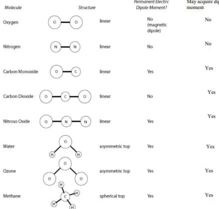
provoked by the different wavelengths of radiation (from Burrows et al., 2011). ... 31 Figure 3.2 - Geometries of important trace gases and dipole moment status (from

http://flux.aos.wisc.edu/~adesai/documents/aos640/AtmosRadCh9-10.pdf). ... 32

Figure 3.3 - Axes in red of rotational freedom for linear diatomic and triatomic and asymmetric top molecules and some examples (from Socolik, 2009). Diatomic molecules show two degrees of rotational freedom and asymmetric top three and respectively the same number of inertia moments. ... 33 Figure 3.4- Vibrational modes of diatomic and triatomic atmospheric molecules (from

http://flux.aos.wisc.edu/~adesai/documents/aos640/AtmosRadCh9-10.pdf). ... 34

Figure 3.5- Vibrational-rotational transitions for  1, J



1,0,1



and illustration of the transitions in the spectrum. P and R branches correspond, respectively, to transitions involving J1 and J1 (from Liou, 2002) . ... 35

Figure 3.6- Scheme for the electronic, vibration and rotation energy levels (from

www.google.com/webhp?nord=1#nord=1&q=+http:%2F%2Fflux.aos.wisc.edu%2F~adesai %2Fdocuments%2Faos640%2FAtmosRadCh9-10.pdf)... 35

Figure 3.7- Potential energy curves for two electronic states of a diatomic molecule. Molecules can be excited into a dissociation level (e.g. transition 1) or into a specific vibrational level of the upper electronic state (e.g. transition 2) (from Liou, 2002). ... 36

(12)

vi Figure 3.8 - Low resolution solar irradiance at top of atmosphere and at sea level and

atmospheric absorption for average atmospheric conditions and an overhead sun (from Palazzi, 2000). ... 39 Figure 3.9- Spectral distribution of the absorption cross section of O2 and O3 adapted (from

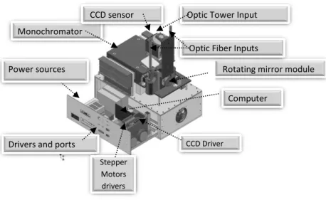
Haigh, 2007). ... 40 Figure 4.1-General Plan of Remote Sensing techniques (from Strong,2005) ... 47 Figure 4.2 - Representation of the main modules of the SPATRAM Instrument. ... 48 Figure 4.3- a) The location of Évora city in mainland Portugal. b) The container in the

Observatory of the Geophysics Centre of Évora in Évora (38.5ºN; 7.9 ºW, 300 m a.s.l.). c) The SPATRAM instrument installed inside the container. ... 49 Figure 4.4 – VELOD a) optical layout; b) project design with the vacuum proof box and the optic fibre. The arrows specify the direction of the input and output of the radiation. ... 50 Figure 4.5- The MIGE platform installed on the roof of the container where the SPATRAM

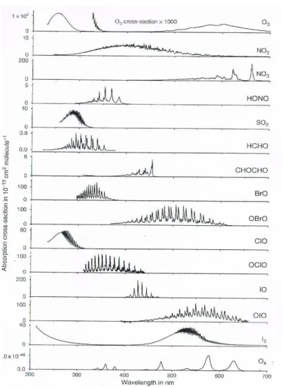
instrument is placed. This platform ensure the possibility to carry out measurements in off-axis configuration along many azimuthally directions since the horizon line is almost completely free (from Domingues, 2011). ... 51 Figure 4.6- Absorption cross sections in cm-2_{of some trace gases from (Platt & Stutz, 2008). . 56}

Figure 4.7- Intensity of monochromatic radiation that crosses the atmosphere (

1 ,S

I ) at

twilight (AM or PM) versus the intensity of monochromatic radiation at local noon (

I

__,₀) obtained with SPATRAM for Ozone measurements. ... 60 Figure 4.8- Plot of ln



I0(,min) Is(,)



versus wavelength for UV spectral range (orange) and

the smoothing function (brown). ... 61 Figure 4.9- “Smoothing” process which consists in filtering the high frequency features in the

spectral data series. The presented values are lnI,0 I,S1ln(I,o/I,S1)versus wavelength (grey)

and ozone differential absorption cross section (red). ... 62 Figure 4.10- Path of radiation (yellow) along the vertical direction for Solar Zenith Angles (SZA)

inferior to 90º (upper panel) and superior to 90º (from Bortoli, 2005). ... 64 Figure 4.11- Illustration of the zenith sky and off-axis viewing geometry. It is possible to see the enhancement of absorption path length in the troposphere due to several off-axis viewing direction near the horizon (adapted from Heckel et al., 2005). ... 69 Figure 4.12- Ratio of the signal obtained by the spectrometer and its “exposure” time (Flux

Index in ms/ digital counting) calculated at the Évora station for a clear sky day and cloudy day. ... 71 Figure 5.1- (Left Panel) Location of the Évora station in the South Western part of the Iberian

Peninsula; (Right Panel) Évora city. SPATRAM + MIGE positioning at the Observatory of the Geophysics Centre of the University of Évora (adapted from Bortoli et al, 2009). ... 79 Figure 5.2- Time series of the O3 Slant Column Density (SCD) in molecules/cm2 obtained with the

SPATRAM equipment installed at Évora Observatory for the 19th_January

2007……….………81 Figure 5.3- O3 Slant Column Densities (SCD) values and Air Mass Factor (AMF) versus time for

the 19th_{January 2007 over Évora retrieved from SPATRAM}

measurements………82 Figure 5.4- O3 VCD for the 19th January 2007 over Évora retrieved from SPATRAM

measurements………..……82 Figure 5.5- Time series of the O3 VCD obtained with the SPATRAM equipment installed at Évora

(13)

vii Observatory during March 2008 - March 2009 period……….…...……….83 Figure 5.6- Full time series of the O3 VCD obtained with the SPATRAM equipment installed at

Évora Observatory during 2007-2011, and the O3 data from the OMI (TOMS) - OMTO3

instrument aboard the NASA EOS- Aura Satellite………....…85 Figure 5.7- a) Filtered time series of the O3 VCD obtained with the SPATRAM equipment at Évora

during 2007-2010, and the O3 data from the OMI (OMI-TOMS) b) Scatter plot of the O3 data

from the OMI instrument (OMI-TOMS OMTO3 product) aboard the NASA EOS – Aura satellite versus O3 SPATRAM data retrieved at Évora Observatory during 2007 – 2011

period………...86 Figure 5.8- Full time series of the O3 VCD obtained with the SPATRAM equipment installed at

Évora Observatory for the SZA of 87º, during 2007-2011, and the O3 data from the OMI

(DOAS) instrument aboard the EOS- Aura Satellite...87 Figure 5.9- Filtered time series of the O3 VCD obtained with the SPATRAM equipment at Évora

during 2007-2010, and the O3 data from the OMI (OMI-DOAS). b) Scatter plot of the O3 data

from the OMI instrument (OMI-DOAS OMDOA3 product) aboard the NASA EOS – Aura satellite versus O3 SPATRAM data retrieved at Évora Observatory during 2007 – 2011

period……….………....……….…..88 Figure 5.10- Full time series of the O3 VCD obtained with the SPATRAM equipment installed at

Évora Observatory during 2007-2010, and the O3 data from the SCIAMACHY instrument

aboard the ENVISAT satellite……….……….……….…….90 Figure 5.11- a) Filtered time series of the O3 VCD obtained with the SPATRAM equipment at

Évora during 2007-2010, and the O3 data from the SCIAMACHY. b) Scatter plot of the O3

data from the SCIAMACHY instrument (TOSOMI product) aboard the ENVISAT satellite versus O3 SPATRAM data retrieved at Évora Observatory during 2007 – 2011

period……….………..91 Figure 5.12- Full time series of the O3 VCD obtained with the SPATRAM equipment installed at

Évora Observatory during 2007-2010, and the O3 data from the GOME instrument aboard

the ERS-2 satellite……….……….……….………92 Figure 5.13- a) Filtered time series of the O3 VCD obtained with the SPATRAM equipment at

Évora during 2007-2010, and the O3 data from the GOME. b) Scatter plot of the O3 data

from the GOME instrument aboard the ERS-2 satellite versus O3 SPATRAM data retrieved

at Évora Observatory during 2007 - 2011 period including the regression line (black line)……...……….…….93 Figure 5.14 - NO2 Slant Column Densities (SCD) and AMF versus SZA obtained with SPATRAM at

Évora-Portugal for 24th_{April 2010. ... 96}

Figure 5.15- Daily variation of NO2 VCD obtained with SPATRAM at Évora-Portugal for 24th April

2010.. ... 97 Figure 5.16- Time series of the NO2 VCD obtained with the SPATRAM equipment installed at

Évora Observatory for the SZA of 90º, during 2007-2011. ... 98 Figure 5.17 - Time series of the NO2 VCD obtained with the SPATRAM equipment installed at

Évora Observatory for the SZA of 90º, during 2007-2011, and the NO2 total columns

acquired from the SCIAMACHY spectrometer aboard ENVISAT. ... ..99 Figure 5.18 - Scatter plot of the NO2 data from the SCIAMACHY instrument versus NO2

SPATRAM AM (morning) and PM (afternoon) data retrieved at Évora Observatory for the SZA of 90º, during 2007 - 2011 period including the regression lines for each dataset….100 Figure 5.19 - Time series of the NO2 VCD obtained with the SPATRAM equipment installed at

Évora Observatory for the SZA of 90º, during 2007-2011, and the NO2 total columns

(14)

viii Figure 5.20 - Correlation of SPATRAM data retrieved at Évora Observatory for the SZA of 90º,

during 2007-2011, and the NO2 data from the GOME-2 instrument... 102

Figure 5.21- Time series of the NO2 VCD obtained with the SPATRAM equipment installed at

Évora Observatory for the SZA of 90º, during 2007-2011, and the filtered NO2 total

columns acquired from the OMI instrument aboard AURA ... 103 Figure 5.22- Correlation of SPATRAM data retrieved at Évora Observatory for the SZA of 90º,

during 2007-2011, and the NO2 data from OMI instrument. ... 104

Figure 5.23- Correlation of SPATRAM NO2 data (average between AM and PM values) retrieved

at Évora Observatory for the SZA of 90º, during 2007-2011, and the NO2 data from the

SCIAMACHY instrument. ... 104 Figure 5.24- Correlation of SPATRAM NO2 data (average between AM and PM values) retrieved

GOME-2 instrument. ... 105 Figure 5.25- Correlation of SPATRAM NO2 data (average between AM and PM values) retrieved

OMI instrument. ... 105 Figure 5.26 -Time series of the BrO VCD obtained with the SPATRAM equipment for the SZA of

90º, a) for morning (AM) and afternoon (PM) and averaged values for the period 23 January – 2 August 2008 at Évora Observatory and the polynomial fit. ... 106 Figure 5.27- Time series of the BrO VCD obtained with the SPATRAM equipment installed at

Évora Observatory for the SZA of 90º, for morning (AM) and afternoon (PM), for the period 23 January – 2 August 2008, and the BrO total columns measured with the OMI equipment……….107 Figure 5.28- Correlation of SPATRAM BrO data retrieved at Évora Observatory for the SZA of

90º, during 2007-2011, and the BrO data from the OMI instrument… ... 108 Figure 5.29- Time series (all dataset) of the BrO VCD averaged values from morning (AM) and

afternoon (PM) obtained with the SPATRAM equipment installed at Évora Observatory for the SZA of 90º for the period 23 January – 2 August 2008, and the BrO total columns measured with the OMI equipment………..109 Figure 5.30- Correlation of SPATRAM BrO VCD averaged AM and PM datasets retrieved at

Évora Observatory for the SZA of 90º, during 2007-2011, and the BrO data from the OMI instrument. ... 109 Figure 5.31- Time series (filtered dataset) of the BrO VCD averaged values from morning (AM)

and afternoon (PM) obtained with the SPATRAM equipment installed at Évora

Observatory for the SZA of 90º for the period 23 January – 2 August 2008, and the BrO total columns measured with the OMI equipment. ... 110 Figure 5.32- Correlation of SPATRAM BrO VCD averaged AM and PM and filtered datasets

retrieved at Évora Observatory for the SZA of 90º, during 2007-2011, and the BrO data from the OMI instrument. ... 111 Figure 5.33- Time series of the BrO VCD obtained with the SPATRAM equipment installed at

Évora Observatory for the SZA of 90º, for morning (AM) and afternoon (PM), for the period 23 January – 2 August 2008, and the BrO total columns measured with the GOME-2 equipment……….………11GOME-2 Figure 5.34- Time series (all dataset) of the BrO VCD averaged values from morning (AM) and

(15)

ix the SZA of 90º for the period 23 January – 2 August 2008, and the BrO total columns measured with the OMI equipment... ..113 Figure 5.35- Correlation of SPATRAM BrO VCD AM and PM datasets retrieved at Évora

Observatory for the SZA of 90º, during 23 January – 2 August 2008, and the BrO data from the GOME-2 instrument. ... 113 Figure 5.36- Correlation of SPATRAM BrO VCD averaged AM and PM datasets retrieved at

Évora Observatory for the SZA of 90º, during 23 January – 2 August 2008, and the BrO data from the GOME-2 instrument. ... 114 Figure 5.37- NO2 SCDs during 30 th March 2009 for a zenith elevation of 88° along the a) West,

b) East, c) North and d) South azimuthal direction. ... 115 Figure 5.38- NO2 vertical profiles for 8th April 2009 retrieved a) East b) North azimuthal

direction with an horizontal visibility of 30 km. ... 117 Figure 5.39- NO2 vertical profiles for 9 th April 2009 retrieved a) East b) North azimuthal

direction with an horizontal visibility of 30 km. ... 118 Figure 5.40- NO2 stratospheric vertical profiles for May of 2010 retrieved with SPATRAM at

Évora Observatory. ... 119 Figure 5.41- NO2 stratospheric vertical profiles for June- August of 2010 retrieved with

SPATRAM at Évora Observatory. ... 120 Figure 5.42- NO2 stratospheric vertical profiles for September and October of 2010 retrieved

with SPATRAM at Évora Observatory... 120 Figure 5.43- NO2 stratospheric vertical profiles for some days of May 2010, comprising the

minimum values, maximum values and the averaged values retrieved with SPATRAM instrument and comparison with SCIAMACHY datasets from Max Plank Institute Mainz (SCIAMACHY MPI) and the Institute of Environmental Physics (IUP/IFE) of University of Bremen (SCIAMACHY Bremen). ... 122 Figure 5.44- NO2 stratospheric vertical profiles for some days of June, July and August 2010,

comprising the minimum values, maximum values and the averaged values retrieved with SPATRAM instrument and comparison with SCIAMACHY datasets from Max Plank Institute Mainz (SCIAMACHY MPI) and the Institute of Environmental Physics (IUP/IFE) of

University of Bremen (SCIAMACHY Bremen). ... 122 Figure 5.45- NO2 stratospheric vertical profiles for some days of September and October of

2010, comprising the minimum values, maximum values and the averaged values

retrieved with SPATRAM instrument and comparison with SCIAMACHY datasets from Max Plank Institute Mainz (SCIAMACHY MPI) and the Institute of Environmental Physics

(IUP/IFE) of University of Bremen (SCIAMACHY Bremen). ... 123 Figure 5.46 a) The NO2 Slant Column Densities (SDC) daily variation during 11th May of 2010

retrieved by SPATRAM at Évora. b) The HYSPLIT back-trajectories for the 11th_{May of 2010}

at the heights of 1000, 3000 and 5000 m (at

http://ready.arl.noaa.gov/hysplit-bin/trajtype.pl?runtype=archive). ... 126 Figure 5.47- Location of the potential pollution sources (Setúbal, Barreiro, Seixal, Lisboa,

Amadora) detected by the combination of SPATRAM data and HYSPLIT back-trajectories for the 11th_{May of 2010 at the heights of 1000, 3000 and 5000 m- at}

www.maps.google.com...127 Figure 5.48 - Number of pollution events registered at Évora’s Observatory in 2010 with the

(16)

x Figure 5.49- The NO2 Slant column densities (SDC) daily variation during 12th June of 2010

retrieved by SPATRAM at Évora. ... 128 Figure 5.50 - The HYSPLIT back-trajectories for the 12th_{June of 2010 (ending at 13 UTC) at the}

heights of 1000, 3000 and 5000 m (at

http://ready.arl.noaa.gov/hysplit-bin/trajtype.pl?runtype=archive) ... 128 Figure 5.51- The NO2 Slant column densities (SDC) daily variation during the 2nd of March 2010

retrieved by SPATRAM at Évora. ... 129 Figure 5.52- The HYSPLIT back-trajectories for the 2nd_{March of 2010 (ending at 17 UTC) at the}

heights of 10000, 15000 and 25000 m (at

http://ready.arl.noaa.gov/hysplit-bin/trajtype.pl?runtype=archive). ... 129

Figure 5.53- The HYSPLIT back-trajectories for the 2nd_{March of 2010 at the heights of 1000,}

3000 and 5000 m (at http://ready.arl.noaa.gov/hysplit-bin/trajtype.pl?runtype=archive). ... 130 Figure 5.54- Number of pollution events registered at Évora’s Observatory in 2010 with the

potential sources located in Spain. ... 130 Figure 5.55- Histogram that illustrated the quantity of NO2 detected in Évora in µg/m3 with the

SPATRAM instrument for each pollution event, for the 115 events recorded at Évora Station. ... 131

(17)

xi

List of Tables

Table 2.1 - Permanent gases in atmosphere and their mixing ration volume in dry unpolluted air

(adapted from Brasseur et al. 1999). ... 7 Table 2.2 - Trace gases in atmosphere and their mixing ration volume in dry unpolluted air (adapted

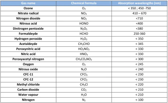
from Brasseur et al., 1999). ... 8 Table 2.3 - Tropospheric major sources, mixing ratios in clean atmosphere, major sinks and atmospheric lifetime of some nitrogen, sulphur, carbon, nitrogen and halogen atmospheric compound species (adapted from Brasseur & Solomon, 2005; Platt & Stutz, 2008). ... 13 Table 3.1 - Wavelengths of absorption in the UV- Visible range by several atmospheric gases (adapted

from Jacobson, 1999). ... 38 Table 4.1 - Observable species detected with SPATRAM and their respective spectral range and ID and

optical ... 60 Table 5.1- O3 total columns maximums and minimums values obtained with SPATRAM ± 1 standard

deviation from OMI- DOAS for the period 2007-2011 over Évora-Portugal... 88 Table 5.2 - Correlation analysis of SPATRAM, OMI (TOMS), OMI (DOAS), GOME and SCIAMACHY total

ozone data for the period of 2007-2011. ... 94 Table 5.3- NO2 total columns maximums and minimums values obtained with SPATRAM ± 1 standard

deviation from SCIAMACHY for the period 2007-2011 over Évora-Portugal. ... 101 Table 5.4- Correlation analysis of SPATRAM, OMI, GOME-2 and SCIAMACHY total nitrogen dioxide data

for the period of 2007-2011. ... 106 Table 5.5- Correlation analysis of SPATRAM (averages AM and PM values) and OMI total BrO data for the

(18)

(19)

xiii

“Aperfeiçoamento de algoritmos para avaliação da qualidade do ar e da composição

atmosférica a partir de medidas de radiâncias espectrais”

Resumo

O principal objetivo deste trabalho consiste na aplicação e aperfeiçoamento de algoritmos numéricos para a inversão de medidas espectrais feitas com um instrumento de deteção remota instalado no Observatório do Centro de Geofísica de Évora (38.6ºN, 7.9ºW, 300 a.s.l.). Os algoritmos explorados são os seguintes: i) metodologia DOAS para a determinação da concentração média de compostos atmosféricos ao longo do caminho ótico, ii) duas diferentes abordagens ao algoritmo de inversão de Chahine que consiste num método iterativo para a obtenção dos perfis dos constituintes atmosféricos minoritários usando o output da técnica espetral. Os resultados obtidos permitiram a avaliação dos ciclos diurnos e sazonais e de variações anuais das colunas totais de ozono, dióxido de azoto e de óxido de bromo, dos perfis verticais de dióxido de azoto e informação acerca de massas de ar poluídas no período compreendido entre 2007-2011. As quantidades obtidas são comparadas/validadas com os respectivos resultados obtidos com instrumentos instalados em satélites.

“Improvement of algorithms for the assessment of air quality and atmospheric

composition from observations of spectral radiances”

Abstract

The central part of this work is the application and improvement of numerical algorithms for the inversion of spectral measurements carried out with a remote sensing instrument, installed at the Geophysics Centre of Évora´s Observatory (38.6ºN, 7.9ºW, 300 a.s.l.).The exploited algorithms are: i) the Differential Optical Absorption Spectroscopy method, for the determination of the mean concentration of an atmospheric compound along an optical path; ii) two different approaches to the Chahine inversion algorithm that is an iterative method for proﬁle retrieval of atmospheric tracers using the output of the spectroscopic technique. The obtained results allow for the assessment of diurnal cycles, seasonal and inter-annual variations for the total columns of ozone, nitrogen dioxide and bromine oxide, the atmospheric profiles of nitrogen dioxide and information about nitrogenous air masses transported over Évora for the period 2007-2011. In addition, the retrieved quantities are compared/ validated with analogous results obtained with satellite borne instruments.

(20)

(21)

xv

Extended Abstract

The atmospheric composition and structure play a key role on the climate system. Atmospheric tracers and aerosols affect climate by altering incoming solar radiation and out- going infrared radiation that are part of Earth’s energy balance. Since the start of the industrial era, the overall effect of human activities on climate has been a warming influence. The human impact on climate during this era greatly exceeds that due to known changes in natural processes, such as solar changes and volcanic eruptions. In this frame, this PhD work tries to clarify the present atmospheric composition, the modifications occurred in the last centuries in our climate system and the main role played by the gaseous atmospheric tracers(ozone, nitrogen and bromine oxides) with the presentation of their main chemical cycles in the atmosphere. Moreover, the central part of this work is the application and improvement of numerical algorithms for the inversion of spectral measurements carried out with the SPATRAM (SPectrometer for Atmospheric TRacers Monitoring) remote sensing instrument, installed at Geophysics Centre of Évora - University of Évora (CGE-UE) (38.6º N, 7.9 W, 300 a.s.l.) in the south of Portugal since 2004. The exploited algorithms are: i) the DOAS (Differential Optical Absorption Spectroscopy) method, for the determination of the mean concentration of an atmospheric compound along an optical path; ii) two different approaches to the Chahine inversion algorithm that is an iterative method for proﬁle retrieval of atmospheric tracers using the output of the DOAS technique. The obtained results allow for the assessment of diurnal cycles, seasonal and inter-annual variations for the total columns and atmospheric profiles of ozone, nitrogen and bromine oxides. In addition, the retrieved quantities are compared/validated with analogous results obtained with satellite borne instruments. The analysis is performed for the period 2007-2011. This study also provides information about nitrogenous air masses transported over Évora, in 2010. The joint action of the SPATRAM data and HYSPLIT (HYbrid Single-Particle Lagrangian Integrated Trajectory) maps, allowed for the identification of possible sources responsible for the pollution events recorded at the city.

(22)

(23)

xvii

Acronyms

AERONET = AErosol RObotic NETwork

AMEFCO = Atmospheric MOdel for Enhancement Factor COmputation AMF = Air Mass Factor

APA = Agência Portuguesa do Ambiente

BASCOE= Belgian Assimilation System of Chemical Observations from ENVISAT BIRA- IASB= Belgian Institute for Space Aeronomy

BL= Boundary Layer

CCD = Charged Coupled Device CFC = Chlorofluorocarbons

CGE-UE = Geophysics Centre of Évora – University of Évora DAS = Data Acquisition System

DLR= German Aerospace Centre

DOAS = Differential Optical Absorption Spectroscopy DSCD= Differential Slant Column Density

DU = Dobson Unit

ECU = Electronic Control Unit

ENEA = Italian National Agency for New Technology, Energy and Environment ENVISAT = ENVIronmental SATellite

EOS= Earth Observing System ERS-2= European Remote Sensing 2

EUMETSAT= European Organisation for the Exploitation of Meteorological Satellites FI = Flux Index

FFT = Fast Fourier Transform

FSSD= Fair Spacing of the Spectral Data FOP = Free Optical Path

FRESCO= Fast retrieval scheme for clouds from the oxygen A-band GAW = Global Atmosphere Watch

GOME = Global Ozone MOnitoring Experiment GOME-2 = Global Ozone MOnitoring Experiment 2

HYSPLIT = HYbrid Single-Particle Lagrangian Integrated Trajectory IR = Infrared

INTA = Atmospheric Sounding Station of the Spanish Institute for Aerospace Technology ISAC-CNR = Institute of Atmospheric Sciences and Climate of the Italian National Research

Council

IPMA = Instituto Português do Mar e da Atmosfera IUP= Institute of Environment Physics

IWOP = Intensity Weighted Optical Path LIDAR= Light Detection and Ranging LOS = Line Of Sights

(24)

xviii

METEOP-A= Meteorological operational satellite A MIGE = Multiple Input Geometry Equipment MODTRAN = MODerate resolution TRANSmittance

NASA= National Aeronautics and Space Administration´s Earth NH = Northern Hemisphere

NMHC = Non Methan Hydrocarbons OEM = Optimal Estimation Method OMs = Ozone Mini-holes

OMI = Ozone Monitoring Instrument OMU= Optical Mechanical Unit OPM = Optical Path of Measurements PAN = Peroxyacetyl Nitrate

PBL= Planetary Boundary Layer PSC= Polar Stratospheric Clouds RADAR= RAdio Detection and Ranging RHS= Reactive Halogen Species RTM = Radiative Transfer Model

SAGE = Stratospheric Aerosol and Gas Experiments

SCIAMACHY = Scanning Imaging Absorption Spectometer for Atmospehric Chartography SPATRAM= SPectrometer for Atmospheric Tracers MOnitoring

SC= Slant Column

SH = Southern Hemisphere SL = Sea Level

SOS = Sum Of Squares

SPT = Standard Temperature and Pressure SPE = Solar Proton Events

SST = Total Sum of Squares SSR = Regression Sum of Squares SVD = Singular Value Decomposition SZA = Solar Zenith Angle

TC= Total Column

TOA = Top of the Atmosphere TOC = Total Ozone Columns

TOMS = Total Ozone Mapping Spectrometer UV= Ultraviolet

VC= Vertical Column

VCD = Vertical Column Density VSA = Var Slant Absorber

VOC = Volatile Organic Compound

WMO = World Meteorological Organization

(25)

xix

List of principal symbols

)

(





_a ...absorption coefficient (m -1₎

)

(





_s ...scattering coefficient (m1₎

)

(





_a ...absorption cross section of the absorbing molecule/atom (m2₎

g



...absorption cross section of the gas (m 2₎

)

(





_s ...scattering cross section of the molecule/particles (m 2₎

R



...Rayleigh scattering coefficient (m 2₎





...mass extinction cross section for radiation of wavelength λ (

m /

2

kg

) 



...monochromatic optical thickness( -) n ...number of absorbers (atoms) per unit of volume (m -3₎

S ... scattering function (-)

C ...number of molecules by unit volume ( 3

/ m

molecules )



... solar zenith angle (º)

min

 ………..………. solar zenith angle reached at the local noon (º)

mul

S



... mean photon path into the lth_{layer (cm)}

ρ ...density of the material (

kg

/ m

3)

g



... gas concentration (molecules/cm3₎

a



...density of the air in the i shell (molecules/cm3₎ N ...refractive index (-)



I

...intensity of the incident radiation (W.m2..sr1.



m 1) 

J

... monochromatic source function (W.m2..sr1.



m 1)

1 ,S

I_ ..intensity of monochromatic light that crosses the atmospheric path(W.m2..sr1.



m 1) )

, ( _min 0 

I ……….reference spectrum obtained at local noon (W.m2..sr1.



m 1) )

, (

s

I ………….………spectrum measured for different condition of SZA (W.m2..sr1.



m 1)

)

(

0



I

... intensity of the radiation at TOA (W.m2..sr1.



m 1)

M...air mean molar mass (0.02897 kg/mol)

g... ...acceleration of gravity ( 9.8 m/s2₎ E...Energy of a photon (J)

(26)

xx

h...Planck´s constant ( 6.6236176x10-34_Js)

c...velocity of light in vacuum ( 2.9979x108 m/s2₎

(27)

1

1. Introduction

1.1 State of the art

During the last two centuries the composition of atmosphere has undergone dramatic changes due mainly to the role of human activities (Valks, 2003; IPCC, 2007; WMO, 2003; IPCC, 2013). The main causes for these variations may be identified as the quasi-exponential growth in population that impelled the development of industrialization and energy production, the intensification of both terrestrial and air traffic, the agriculture practices (that include the use of fertilizers and biomass burning) that contribute to the degradation of the air quality on a global scale. The emission of trace gases like nitrogen oxides (NOx), methane (CH4),

chlorofluorocarbons (CFC´s), carbon dioxide (CO2), carbon monoxide (CO), sulphur dioxide (SO2)

and other hydrocarbons compounds resulted in several environmental changes mediated through the chemistry of the atmosphere. These changes have direct impact on the environment and currently we are facing their consequences. Some of these changes include (IPCC 2007; WMO, 2003; Brasseur et al., 1999):

• the rising in global mean temperature (enhancement of the greenhouse effect) resulting from increasing emissions of CO2 and other greenhouse gases,

• global increase of atmospheric pollution,

• the increasing of the concentration of tropospheric oxidants and impacts on the biosphere and human health,

• depletion on the stratospheric ozone over Antarctica during austral spring and ozone mini-holes at the mid-latitudes that cause an increase in UV-B radiation and impacts on living species,

• occurrence of acid precipitation and their impact on the biosphere,

• changes in the self-cleaning capability of the atmosphere and in the residence time of anthropogenic trace gases,

• land use and its impact in environment, • perturbations of the biogeochemical cycles.

By the mid-1990s the attention of the world community has become focused on new range of global environmental problems. Maybe triggered by the discover of “Ozone Hole” in Antarctica

(28)

2 in 1985, the human community in general become more conscious of environmental questions that started to arise like the climate change and (at the time) possible global warming. With the beginning of the twenty-first century the awareness of these problems by the majority of people, leads to the concerning about quality of life. The increasing interest on the study of those problems is related mainly with their adverse effects on health and ecosystems (Zabalza et al., 2007; Zujic et al., 2009).

The rapid acceleration of the concern about those questions led to real advances in related technologies for the acquisition and processing of environmental data in “real or near real-time”, even from remote locations. This progress provides the assessment of data related to the atmosphere and climate, like trace gases and aerosol concentration and clouds, besides the dynamic and meteorological information of the atmosphere (Laj et al. 2009). Nowadays the monitoring of the atmosphere is carried on by means of ‘in-situ’ and Remote Sensing (RS) measurements obtained from ground-based instruments, balloons, airborne or satellite based equipments. The data-sets acquired with all these instruments and sensors enable the monitoring of the atmosphere and can be kept for present and future prospect studies. In a so complex system as the Earth’s Atmosphere compared by Seinfeild et Pandis, 2006 “to an enormous chemical reactor in which a myriad of species are continually being introduced and removed over a vast array of spatial and temporal scales” the need of short and long term observations are evident since atmospheric processes are still far from being entirely understood.

In 1924, Gordon Dobson (25 February 1889 - 11 March 1976) developed the first instrument that allowed for the measurements of atmospheric total ozone: the Dobson Spectrophotometer. Dobson is globally recognized as a great scientist not only for the invention of the equipment with his name, but also for the idea he had to establish a network of these kind of instruments. During the winter of 1925/26 he built the equipment that was installed at the Arosa observatory (Switzerland) known for more than 80 years of continuously measurements. Nowadays a network of about 90 Dobson Spectrometers are spread all over the world taking trust worthy measurements for the WMO's global ozone observing network run as part of the Global Atmosphere Watch (GAW). Currently, other ground based spectrometers fully automatic are operating around the world (Meena, 2009) and the reference instrument for ozone measurements is the Brewer spectrometer that basically is the automated version of the Dobson equipment.

With the development of Dobson´s spectrometer the atmospheric inverse problems emerge consequently. At the beginning, the measurements made by Dobson were based on the absorption of solar UV light and he was able to retrieve O3 total column contents. Approximately

(29)

3 10 years later, Götz realized that it was possible to obtain the vertical distribution of that gas by measuring the Rayleigh scattered sunlight from the zenith sky with the same spectrometer. It was the first stone on the development of the so-called Umkehr method (from the German reversal method) (Mateer,1964) for which several scientists contributed for with a huge success. Nevertheless, in the last years, with the appearance of large computers, the launching of earth orbiting satellites observing the atmosphere from outside, the development of new instruments and the improvements of remote sensing techniques the inversion problems received more attention (Twomey, 1996). One of the first efforts to determine the vertical distribution of the temperature in the atmosphere was proposed by Kaplan using satellites as a function of wavelength and later developed by Wark and Yamamoto (Ferral, 2011). In the beginning of atmospheric satellite era the vertical profiles of several gases and aerosols began to be retrieved using the Stratospheric Aerosol and Gas Experiments (SAGE). Several instruments onboard satellites followed such as Global Ozone Monitoring Experiment (GOME), SCanning Imaging Absorption spectroMeter for Atmospheric CHartographY (SCIAMACHY) and Ozone Monitoring Instrument (OMI) using inverse methods for the same purpose.

This work is inserted in the thematic of climate change as well as of air quality since trough the monitoring of trace constituents in the entire atmospheric column it is possible to infer the temporal series of total columns and vertical profiles of trace gases and their changes for a chosen temporal period.

Trace gases are known for their minor concentrations in the atmosphere, but their major role in it. This work is focused on the monitoring of ozone and nitrogen dioxide, which are key species in both stratospheric and tropospheric chemistry. The observations are performed with a UV- VIS ground based spectrometer known as SPATRAM (SPectrometer for ATmospheric TRAcers Monitoring).

1.2 Motivation

The main motivations for conducting this work were:

• the importance of monitoring the trace compounds in the atmosphere;

• the lack of atmospheric chemistry measurements in the south of Portugal and the need for such measurements taken automatically on a routine basis;

• the inexistence of long term studies of total atmospheric column and vertical profiles of NO2 and O3, using ground based spectrometers in Portugal. There are several studies

focusing the air quality monitoring in urban areas conducted by researchers of the University of Aveiro and University of Porto. The published studies are centered in the

(30)

4

in-situ monitoring of trace gases at the surface, such as tropospheric O3, NO2, Volatile

Organic Compounds (VOCs) and Particulate Matter (PM) (Mendes at al., 2008; Alvim-Ferraz et al., 2005; Monteiro et al., 2007; Evtyugina et al., 2006) and in the direct relation with human health impacts (Sousa et al. 2009; Sousa et al., 2008).

• the improvement and use of the SPATRAM equipment. In Portugal there are only available 2 Brewer spectrophotometers installed in Funchal (Madeira Island) and in Angra do Heroísmo (Azores islands) and a Dobson spectrometer which is deactivated at the moment. Their data are available at the World Ozone and Ultraviolet Radiation Data

Centre (WOUDC) platform

(http://www.woudc.org/data/MetaQuery/metaquery_e.cfm) but just until 2003. The Ozone profiles are only taken by the Instituto Português do Mar e da Atmosfera (IPMA) with balloons sondes. The Agência Portuguesa do Ambiente (APA) also supplies the NO2

and O3 measurements but only at the surface (available at http://qualar.apambiente.pt/).

• the fact that Portugal is one of the regions of the European countries with the highest insolation which is a key quantity relevant in the tracers photo-chemistry;

•

the fact that the south of Portugal presents clear sky conditions for early spring to autumn which favours the frequent observations using RS instruments.

1.3 Objectives

The main objectives of this work are addressed to the improvements of the algorithms utilized to invert the spectral measurements of the SPATRAM instrument aiming to increase the accuracy and the confidence in the retrieval of:

• total column concentrations of NO2, O3 and BrO and comparison with satellite data,

• vertical profiles of stratospheric NO2 (from 10- 50 km), with a vertical resolution of 2.5

km,

• vertical profiles of tropospheric NO2 (from the ground till to 2 km of altitude), with a

vertical resolution of 250-300 m ,

over Évora - Portugal (38.6ºN, 7.9ºW, 300 m a.s.l.) for the period comprised between 2007-2011. Furthermore, the synergy between the SPATRAM observations and a dynamical model allowed for the identification of anthropogenic pollution events in the city due to air mass circulation from sites with high pollution loads.

(31)

5

1.4 Thesis structure

This thesis is divided in 6 chapters.

The present composition and structure of the atmosphere is described briefly in chapter 2. In the same section the basic principles of the atmospheric chemistry for ozone, nitrogen dioxide and bromine oxide are presented. Some key aspects of the role of these compounds in the atmospheric processes and some chemical cycles (in particular for ozone) are described. In chapter 3 a brief description of the absorption and scattering processes in atmosphere is presented giving emphasis to the interactions of the gaseous compounds with the solar radiation in UV-VIS bands.

The overview of the remote sensing techniques is given in the first section of chapter 4, followed by the descriptions of the ground-based spectrometer (SPATRAM) and of the satellite borne equipment’s (OMI, SCIAMACHY, GOME, GOME-2) used in this work. The last sections of chapter 4 deal with the spectroscopic technique (DOAS – Differential Optical Absorption Spectroscopy) for the retrieval of the mean content of trace gases along an optical path (SCD – Slant Column Density) from the spectral radiation measurements carried out with the ground based instrument. The DOAS-Master-Equation is derived and the radiative transfer models for the interpretation of the outputs of the DOAS algorithms are presented. Also the inversion methods for the retrieval of the vertical profiles for the studied trace gas using the SCDs values and the output of the radiative transfer models are presented and explained in detail.

The results of this study are presented in chapter 5 in terms of trace gases (O3, NO2 and BrO)

variability, air quality monitoring, and vertical distribution of NO2. In addition, comparisons of

the ground-based results with data obtained with similar satellite borne equipment are shown and discussed. The outlook is presented in chapter 6 as well the future work that can be developed in this field.

(32)

(33)

7

2. Chemistry of atmosphere: the role of

ozone and nitrogen dioxide

2.1 Introduction

The terrestrial atmosphere is a thin layer of gases that surrounds the planet and separates Earth’s surface from space. The atmosphere has several roles in order to support life like the maintenance of temperature, the protection of the earth’s surface from radiation, the removal of some oxidant gaseous compounds and the redistribution of heat and water. This chapter presents some aspects of atmospheric dynamics and composition giving emphasis to the role and to the chemistry of ozone and of nitrogen dioxide in the troposphere and stratosphere.

2.2 Atmospheric composition and structure

2.2.1 Atmospheric composition

Presently the Earth’s atmosphere is composed by a mixture of gases, water vapour and aerosols. The most abundant species in atmosphere are nitrogen (N2), and oxygen (O2). These gases as

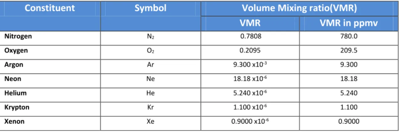
well as noble gases like Argon (Ar), Néon (Ne), Helium (He), Krypton (Kr) and Xenon (Xe) represent permanent gases which are characterized by their almost constant mixing ratios in time and space over short time scales. Most of these gases are situated in a region under 100 km called homosphere. Table 2.1 presents the permanent constituents of dry "unpolluted" air and their mixing ratios in the atmosphere.

Table 2.1 - Permanent gases in atmosphere and their mixing ration volume in dry unpolluted air (adapted from Brasseur et al., 1999).

Constituent Symbol Volume Mixing ratio(VMR)

VMR VMR in ppmv Nitrogen N2 0.7808 780.0 Oxygen O2 0.2095 209.5 Argon Ar 9.300 x10-3 _9.300 Neon Ne 18.18 x10-6 _18.18 Helium He 5.240 x10-6 _5.240 Krypton Kr 1.100 x10-6 _1.100 Xenon Xe 0.9000 x10-6 _0.9000

(34)

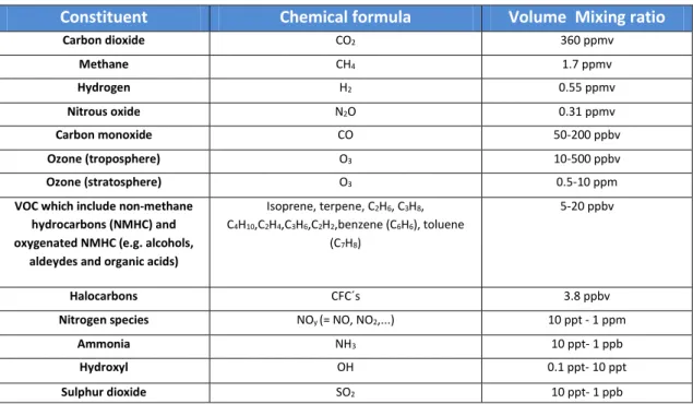
8 The minor part of the atmosphere is composed by several other substances called trace gases. Despite their low concentration in atmosphere they have a very high impact in atmospheric chemistry and climate. Their mixing ratios vary in time and space, although they constitute only ~0.04 % by volume of the atmosphere. For example, trace gases have significant roles in the transmission of solar and terrestrial radiation and in biogeochemical cycles that restrict the atmospheric lifetime of other gases.

Table 2.2 summarizes the volume mixing ratios of trace gases in atmosphere.

Table 2.2 - Trace gases in atmosphere and their mixing ration volume in dry unpolluted air (adapted from Brasseur et al., 1999).

Constituent Chemical formula Volume Mixing ratio

Carbon dioxide CO2 360 ppmv Methane CH4 1.7 ppmv Hydrogen H2 0.55 ppmv Nitrous oxide N2O 0.31 ppmv Carbon monoxide CO 50-200 ppbv Ozone (troposphere) O3 10-500 ppbv Ozone (stratosphere) O3 0.5-10 ppm

VOC which include non-methane hydrocarbons (NMHC) and oxygenated NMHC (e.g. alcohols,

aldeydes and organic acids)

Isoprene, terpene, C2H6, C3H8,

C4H10,C2H4,C3H6,C2H2,benzene (C6H6), toluene

(C7H8)

5-20 ppbv

Halocarbons CFC´s 3.8 ppbv

Nitrogen species NOy (= NO, NO2,...) 10 ppt - 1 ppm

Ammonia NH3 10 ppt- 1 ppb

Hydroxyl OH 0.1 ppt- 10 ppt

Sulphur dioxide SO2 10 ppt- 1 ppb

Figure 2.1 shows a close distribution of the mixing ratio of some atmospheric constituents depending on the altitude. In that figure the N2 and the noble gases are not represented (with

the exception of Argon). The N2 mixing ratio distribution function should be similar to O2 profile

but starting at sea level with a value of ~0.78.

Other important atmospheric constituents are aerosols which are small particles of liquid or solid matter dispersed and suspended in air as for example, water droplets, dust or soot particles. Their sizes range from 0.001 to 1000 µm. The major aerosol species in the atmosphere are nitrate, sulphate, black carbon, organic carbon, sea salt and mineral dust. Aerosols have many roles in the atmospheric chemistry like interactions with radiation and cloud condensation nuclei.

(35)

9

Figure 2.1 - Typical vertical distribution of the concentration of chemical atmospheric constituents under about 120 km (from Liou, 2002.)

2.2.2 Atmospheric vertical structure

The thermal structure of the atmosphere, up to approximately 120 km, can be divided in four layers characterized by different vertical temperature gradients: troposphere, stratosphere, mesosphere and thermosphere (Fig.2.2). The regions are separated by boundaries called pauses: tropopause, stratopause and mesopause, respectively.

Figure 2.2- Temperature variation in Earth’s atmosphere (from Platt & Stutz, 2008).

The troposphere is the first layer which extends from the surface up to about 6-8 km near the poles, 12 km at mid-latitudes and to 18 km at the equator, depending on the water vapour content present in this layer. The troposphere can be sub divided into: i) Planetary Boundary

(36)

10 Layer (PBL) which extends from surface till 1-2 km (depending on the time of the day and meteorological conditions); ii) the free troposphere located between the PBL and the tropopause. The troposphere contains about 85-90% of the atmospheric mass and its temperature profile is mainly explained by the adiabatic expansion and compression of respectively rising and sinking air masses, driven by solar radiation. In this layer occurs all the meteorological phenomena (like rain, snow and wind formation) which are a result of its negative temperature gradient (-5 to -10ºC/km) that originates a region of convective and turbulent mixing. The vertical transport of chemical compounds in the troposphere is controlled by strong vertical mixing (including convection) whereas in the stratosphere this vertical mixing is absent.

The stratosphere is located above the tropopause, which is a layer with a fairly uniform temperature (no change of temperature with altitude) of about 40 km depth, and extends up to 50 km. This level contains 90% of the atmospheric ozone located in a stratum generally referred as “ozone layer” and the vertical temperature is constant till ~20 km and then increases till the stratopause. The absorption of UV radiation by ozone causes temperature rising with altitude in this region. The vertical gases transport in the stratosphere is controlled by the Brewer- Dobson circulation. This circulation was first proposed by Brewer (1949) and Dobson (1956) and consists of a global scale air movement in the stratosphere. This movement is composed by three parts: a) air rises in the tropics from the troposphere into stratosphere b) and then moves poleward in the stratosphere and finally c) descends in both the stratospheric middle and polar latitudes (Forster et al., 2010; Butchart et al., 2006; Roscoe, 2006).

The mesosphere is located between the top of the stratopause and extends till 90 km altitude. In this layer the temperature decreases with height due to similar processes as in the troposphere. In the thermosphere, above the mesopause, the temperature increases to maximum values. Like in stratosphere, there are positive temperature gradients in this layer that indicate that there is a heat source inside the thermosphere which is due to the absorption of the short wavelength solar radiation (UV) by atoms and molecules (mainly oxygen) and by the accumulation of energy and matter resulting from interstellar dust and coronal mass ejection. The pressure and density of air decrease with altitude. The pressure of Earth’s atmosphere obeys the barometric equation (Eq.2.1) and falls exponentially as a function of height as shown

in Figure 2.3. At higher altitudes (z), the atmospheric pressure (p(z) ) varies as follows: p z p e RT z Mgz   0 ) ( (2.1) where M is the air mean molar mass (0.02897 kg mol-1_{), g is the acceleration of gravity}

(9.8 ms-2_{), and z}

(37)

11

Figure 2.3- Variation of atmospheric pressure in Earth’s atmosphere with altitude in the Earth’s atmosphere for tropical regions, mid latitudes in summer and winter, and high latitude sub arctic summer and winter (from Burrows et al., 2011).

2.3 Trace gases in the atmosphere

The atmospheric distribution of trace gases is conditioned by atmospheric transport, dispersion, photochemical reactions and physical removal of these gases. As a consequence, the composition of the atmosphere is directly affected by the balance between addition and removal of its components.

Gases are produced by a) chemical processes in the atmosphere, b) biological activity (exchanges with vegetation, biological organisms and ocean), c) volcanic activity, d) radioactive decay, e) human activities. Gases are removed from the atmosphere also by a) chemical processes in the atmosphere and b) biological activity as well as c) physical processes in the atmosphere, d) deposition (wet and dry deposition) and e) uptake by the oceans and land masses.

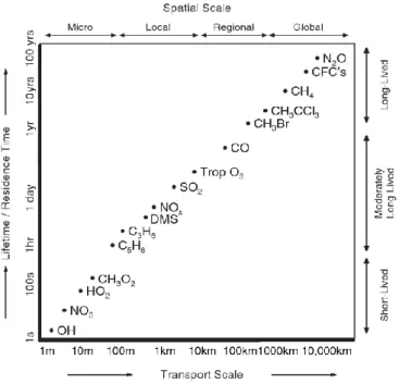
The lifetime of the species is also an important factor taking into account in the removal of gases from the atmosphere. The lifetime is the time period during which the species stay in atmosphere before their removal. There are species that reside in the atmosphere just a few seconds (e.g. OH) whereas others can last for several years (e.g. CFC´s) (Figure 2.4). It is also important to take into account the spatial scales of the atmospheric motions in addition to the removal processes. The atmospheric phenomena can occur in spatial scales varying from 0-100 m (microscale events like urban air pollution), ten to hundreds of kilometres (mesoscale events like land-sea breezes, regional air pollution), hundreds to thousands of kilometres (synoptic scale events like motions of whole weather systems, stratospheric ozone depletion) and large scale events that exceed the 5000 km (global scale/planetary events) (Fig. 2.4).

(38)

12

Figure 2.4- Spatial and temporal scales variability of some atmospheric gases (from Platt & Stutz, 2008).

Concerning to air monitoring it is important to acknowledge sources and sinks of the gaseous and particulate components which are emitted to atmosphere. Most of the species considered air pollutants have natural and anthropogenic sources according to the type of sources involved in gaseous emissions. Natural emission of gases includes the following sources: a) volcanic emissions, b) thunderstorms / lightning, c) soil emissions, d) vegetation emissions, e) biomass burning and f) marine emissions. Anthropogenic emissions are directly related to human activity and include: a) industrial processes, b) fossil fuel and biofuel combustion (e.g. traffic related to vehicles exhausts, power plant stations, c) biomass burning (e.g. deforestation, biomass stations VOCs, CO and NOx), d) agriculture practices (e.g. agricultural land, animals, agricultural waste

burning).

The atmospheric traces constituents can be classified according to their chemical composition in small groups: sulphur, nitrogen, carbon and halogen containing compounds. The sources, sinks and lifetimes of the most important trace substances are presented in Table 2.3.

(39)

13

Table 2.3 - Tropospheric major sources, mixing ratios in clean atmosphere, major sinks and atmospheric lifetime of some nitrogen, sulphur, carbon, nitrogen and halogen atmospheric compound species (adapted from Brasseur & Solomon, 2005; Platt & Stutz, 2008).

Gas Chemical

Formula

Mixing Ratios Major Sources Major Sinks Atmospheric

lifetime

Nitrogen coumpounds

Nitrous oxide N2O 310 ppb (Tropical) Soil emission , ocean emission,

anthropogenic (mainly from artificial fertilizers and chemical industry)

Loss to stratosphere 110 yr

Nitrogen oxides NO

NO2

0.03 - 5 ppb Fossil fuel combustion, biomass burning, soil emission, microbial production, thunderstorms, aircraft emissions

Oxidation by OH, O3 and

HNO3

~2d

Amonia NH3 ~0.1ppb marine

~5 ppb continent

Livestock wastes, emission from vegetation, ocean emission, fertilized soils, modern cars with catalytically converters. Dry deposition, conversion to NH4+ aerosol. ~5 d Sulphur compounds Sulphur dioxide SO2 0.02-0.09 ppb marine 0.1-5 continent

Fossil fuel burning, volcanoes, sulphide oxidation Dry deposition, reaction with OH, liquid phase oxidation to SO4 =+wet

deposition

~4 d

Hydrogen sulphide H2S 0.005-0.09 ppb Soil emission, vegetation, volcanoes Reaction with OH ~3 d

Dimethyl sulphide DMS

CH3SCH3 0.005-0.1 ppb Soil and ocean emissions Reaction with OH, NO3,

BrO

~2 d

Carbonyl sulphide COS 0.5ppb Soil emission Uptake by vegetation 7 yr

Carbon containing species

Carbon dioxide CO2 Combustion, ocean, biosphere

Methane CH4 1700 ppb Rice fields, domestic animals, biomass burning,

fossil fuel consumptions, swamps

Reaction with OH, export to stratosphere, Soil uptake

~8 yr

Carbon monoxide CO 200 ppb (N.

Hemisphere)

Anthropogenic emission- fossil fuels, biomass burning, CH4 and natural VOC oxidation

Reaction with OH, Flux to stratosphere, soil uptake VOC alkanes ~40-45%, alkenes ~10%, aromatic hydrocarbons ~20% and oxygenates ~10-15% Isoprene (C5H8) Terpenes (C10H16) etc. 0.6-2.5 ppb 0.03-2 ppb

Emission for deciduous trees Emission for coniferous trees

Fossil fuel (emissions from motor vehicles due to either evaporation or incomplete combustion of fuel), biomass burning, foliar and ocean emission

Reaction with OH, ozonolysis

~0.2 d ~0.4 d

Halogens compounds (some examples) Chlorofluorocarbons, (CFC)

Hydrohlorofluorocarbons(HCFC) Hydrofluorcarbons (HFC)

Anthropogenic (their production is now banned, except for HFC)

- -

Halons (bromine and fluorine compounds) Anthropogenic (their production is now banned) - -

Methyl cloride CH3Cl ~550 ppt (Brasseur

et al.,1999)

Industrial processes, biomass burning, oceans, wetlands and wood-rot fungi, tropical and subtropical forests (Rhew, 2011)

oxidation by hydroxyl and chlorine radicals as the dominant sink, followed by loss to polar ocean waters and degradation in soils

1 yr (Rhew, 2011)

Methyl bromine CH3Br 10-15 ppt

(Brasseur et al., 1999)

Biological activity in the ocean, emissions from fumigation(soils, quarantine and reshipment), surface oceans, biomass burning, exhaust from automobiles using leaded gasoline combustion, wetlands, brassica crops, and fungus (Cox et al., 2005; Rhew, 2011)

oxidation by hydroxyl radical, followed by chemical and biological degradation in the oceans and biological degradation in soils

0.8yr (Rhew, 2011)

Methyl Iodine CH3I ~1-10 ppt (Brasseur

et al.,1999) ~1-3 ppt and 10-40 ppt (Cox et al., 2005)

Ocean emissions (Voght et al., 1998), biomass burning, rice paddies, soil bacteria (Youcouchi et al., 2008), rice production and peatland/wetland ecosystems (Cox et al.,2005)

3-5 d (Cox et al., 2005)

Improvement of algorithms for the assessment of air quality and atmospheric composition from observations of spectral radiances

Tese apresentada à Universidade de Évora

para obtenção do Grau de Doutor em Ciências da Terra e do Espaço.

Especialidade: Física da Atmosfera e do Clima.

Ana Filipa Alves Real Domingues

IMPROVEMENT OF ALGORITMS FOR

THE ASSESSMENT OF AIR QUALITY

AND ATMOSPHERIC COMPOSITION

FROM OBSERVATION OF SPECTRAL

RADIANCES

Tese apresentada à Universidade de Évora

para obtenção do Grau de Doutor em Ciências da Terra e do Espaço

Especialidade: Física da Atmosfera e do Clima

Ana Filipa Alves Real Domingues

IMPROVEMENT OF ALGORITMS FOR

THE ASSESSMENT OF AIR QUALITY

AND ATMOSPHERIC COMPOSITION

FROM OBSERVATION OF SPECTRAL

RADIANCES

Acknowledgments

Contents

List of Figures





I





List of Tables

“Aperfeiçoamento de algoritmos para avaliação da qualidade do ar e da composição

atmosférica a partir de medidas de radiâncias espectrais”

Resumo

“Improvement of algorithms for the assessment of air quality and atmospheric

composition from observations of spectral radiances”

Abstract

Extended Abstract

Acronyms

List of principal symbols

)

(





)

(





)

(







)

(









m /

kg





S



kg

/ m





I



J









)

(



I



1. Introduction

1.1 State of the art