Electrical energy supply for Rio Grande do Sul, Brazil, using forecast combination of weighted eigenvalues

(1)

Abstract

The technique of forecast combination (FC) can achieve results superior to those generated by individual forecasting techniques. The purpose of this research is to present a method of FC based on the principal component analysis (PCA) applied to forecast values originating from individual forecasting models such as ARIMA, ARFIMA and SARIMA and their variants. From the PCA, it is possible to weigh up the values from each individual model in order to obtain a linear combination which represents all characteristics of valid models for each supplier. As an example, the FC method proposed was applied in the industrial sector of the three largest electric power suppliers in the State of Rio Grande do Sul, Brazil. The proposed method proved to be very useful since it presented better results than the individual models.

Keywords: Forecast combination; electricity supply distribution; forecast; principal component analysis.

do Sul, Brazil, using forecast combination

of weighted eigenvalues

Adriano Mendonça Souza, (DE, UFSM – RS/Brasil) - amsouza@smail.ufsm.br • Departamento de Estatística (CCNE), sala 1205c

Av. Roraima, 1000, Cidade Universitária, Camobi, 97105-900, Santa Maria-RS, fone: (55) 55-3220-8486 Francisca Mendonça Souza (PPGEP, UFSM – RS/Brasil) - kikamatcom@gmail.com

Nuno Ferreira (ISCTE, IUL – BS – Lisboa/Portugal) - nbf@netcabo.pt Rui Menezes (ISCTE, IUL – BS – Lisboa/Portugal)

(2)

GEPROS.

Gestão da Produção,

Operações e Sistemas – Ano 6,

nº 3,

Jul-Set/2011,

p

. 23-39

1. INTRODUCTION

The technique of forecast combination (FC) was originally developed by Bates & Granger (1969), who demonstrated that FC can achieve results superior to those generated by individual forecasting techniques. FC is a technique that helps to increase the accuracy of forecasts by capturing information and features which individual models fail to achieve (MAKRIDAKIS & WINKLER, 1983; LIBBY & BLASHFIELD, 1978).

According to Rausser & Oliveira (1976), the importance of FC goes beyond simply improving the accuracy and a reduction in the forecast error variance (WERNER, 2004). This is because it is quite common to find a more representative model of the series and also because we have to choose one specific model instead of various ones. When discarding a model in favor of another, some useful information may be also discarded. The FC can avoid this trade-off. It is therefore advisable to consider various techniques and combine them rather than consider just a single technique for forecasting.

Although the FC presents conditions of predictability better than the individual models, accor-ding to Clemen (1989), the ideal conditions to set a combination are not established and the most efficient method in any given situation is not known.

Therefore, the purpose of this research was to present a method of FC based on the principal component analysis (PCA) applied to the forecast values originating from the individual forecasting models. From the PCA, it is possible to weigh the values from each individual model. The FC method proposed was applied in the industrial sector for the three largest electric power distributors in the state of Rio Grande do Sul (RS), Brazil.

Electrical energy supply forecasts within the industrial sector are very important because deci-sions may be taken under different forecast scenarios which require the estimated values closest to the actual values.

This paper is organized as follows: section 2 presents the model predictions used for individual forecasting and PCA; section 3 presents the methodology; section 4 shows the applications and discus-sion, and section 5 presents the conclusions.

2. BACKGROUND

In this section, the forecasting models and PCA are described in order to support the proposed methodology, likewise to implement the FC presented.

(3)

Gestão da Produção,

Operações e Sistemas – Ano 6,

nº 3,

Jul-Set/2011,

p

. 23-39

2.1. Forecasting models

Autoregressive integrated moving average (ARIMA) models are based on the theory that the behavior of the variable itself may answer for their future dynamics (BOX & JENKINS, 1970).

The parameter estimation is usually performed using the method of Minimum Least Squares or Maximum Likelihood and residual diagnostic tests are performed to validate the model and to enable it to predict.

Generally, a non-stationary process ARIMA (p, d, q) follows the eq. 1.

(1) ϕ(B) Δd_X

t = θ(B)at

where, B is the retroactive operator, d represents the order of integration, ϕ is the term represented by the autoregressive order p, θ is the parameter of moving average represented by q, and at = RB (0;σ2),

which is the white noise.

It is not necessary to use all the filters from the general ARIMA model in order to represent a pro-cess. The series can be described by a purely autoregressive (AR) or moving average (MA). If the series is stationary, the integration order is d = 0, and if the series is non-stationary the order of integration is d = 1 or d = 2. It is important to note that the series must become stationary in order to obtain stable parameter estimates and models able to make predictions.

When a dataset has a repetitive behavior during the period of one year, it is evidence of the seaso-nality effect. Thus, a SARIMA (p, d, q) (P, D, Q) model can be used to catch this behavior. S represents the size of seasonality and P, D, and Q represent the seasonality parameters. The general model is given by the eq. 2.

(2) ϕ(B)Φ(B)Δd_Δds_X

t = θ(B)Θ(B)at

In this case, the parameters ϕ and Θ represent the seasonal autoregressive portion and seasonal

moving average parameters, respectively, and Δds represents the seasonal differences. The series

diffe-rentiation in seasonal terms also aims to make the series become stationary, allowing the application of Box e Jenkins methodology (FARIAS, ROCHA & LIMA, 2000).

To fill this gap, where the order of integration, i.e., not always the values of d = 1 or d = 2, the alternative is to find a fractional order of integration. The autoregressive fractional integrated moving average (ARFIMA) (p, d*, q) models use fractional integration. These models are a generalization of the ARIMA (p, d, q) models with fractional integration (d ∈ R), which were originally proposed by Granger & Joyeux (1980) and Hosking (1981).

(4)

GEPROS.

Gestão da Produção,

Operações e Sistemas – Ano 6,

nº 3,

Jul-Set/2011,

p

. 23-39

Formally, it is said that a process is ARFIMA (p, d*, q) with d* ∈ (-½, ½), if {xt} is stationary and satisfies the eq. 3.

(3) ϕ(B)(1 – B)d_X

t = θ(B)at

where, at ∼ RB(0,σ2a), ϕ(B) and θ(B) are degrees of polynomials p and q, respectively, and B is the

retro-active operator. Hosking (1981) demonstrated that the stationarity conditions for the ARFIMA model (p, d*, q) are d < 0.5.

ARFIMA models are capable of describing simultaneously the dynamics of both short and long term memory of the fractional processes, where the parameter d should explain the structural corre-lation of high orders.

One characteristic of the long memory series is that the autocorrelation function (ACF) of the original series appears to be non-stationary and the differenced series of order 1 seems to be super-differentiated, i.e., the long memory processes are between I(0) and I(I), resulting in a I(d) with d fractional (FIGUEIREDO & MARQUES, 2009).

The fractional differencing parameter is obtained through binomial expansion, where (1-B)d_with

d ∈ R as in eq. 4 and 5. (4) (1 – B)d₌

∑

∞ j=0 d j (–B) j (5) = 1 – dB – d(1–d) 2! B2 – d(1–d)(2 – d)3! B 3_{– ...}

Details about fractional differencing can be found in Beran (1994). The fractional differencing parameters d range from -1 to 1 and can be interpreted according to Hosking (1981) and Jin & Fréchet (2004) and LI et al. (2007) The parameters of the ARFIMA model are estimated using the Maximum Likelihood Method (ML), as shown in Zivot & Wang (2003). In the estimation process used here it is considered that an initial value of the fractional differentiation parameter d is estimated by the GPH procedure proposed by Geweke & Porter-Hudak ( 1983).

Besides presenting a white noise, the Akaike’s Information Criteria (AIC) is used as a measure of adjustment for choosing the best model since it takes into account the number of estimated parameters eq. 6 (MORETTIN, 2006).

(6)

AIC = T ln(SQR) + 2n

(5)

Gestão da Produção,

Operações e Sistemas – Ano 6,

nº 3,

Jul-Set/2011,

p

. 23-39

Among the measures for the evaluation of forecast errors in the literature, the mean absolute per-centage error (MAPE) (eq. 7), the root mean square error (RMSE) (eq. 8), and Theil-U statistic (eq. 9) are used (DIEBOLD & LOPEZ, 1996).

MAPE = 1 n xi – ˆxixi . 100 (7) (8) RMSE = (xi – ˆxi)2 n (9) U = ∑(xi – ˆxi) 2 N i=1 ∑(xi – ˆxi–1)N 2 i=1

In the above equations, n is the number of forecasts made, xi represents the real value at the instant

i, ˆxi represents the expected value at time i, and ˆxi–1 is the value of the variable under study at time i-1. The Theil-U statistic is an index that measures how the results are better than a naive or trivial forecast. According to Amorim Júnior et al. (2004), the naive forecast indicates that the best estimate for a value for tomorrow is today’s value. If U = 1, the error modeling is larger than the naive error, i.e., the model predictions are not better than a naive forecast. If U < 1, the modeling error is smaller than the naive error, that is, the model is acceptable since the model predictions are better than a naive forecast.

To perform FC for electrical energy supply, the ARIMA, ARFIMA and SARIMA models were used. The best estimations according to expressions 7, 8 and 9 were used to compose the FC.

2.2. Principal Component Analysis (PCA)

The method of PCA was developed by Pearson (1901) and later by Hotelling (1933). This te-chnique has been studied by several authors, such as Morrison (1976), Seber (1984), Reinsel (1993), Jackson (1981) and Johnson & Wichern (1992). The central idea behind this method is to reduce the dimensional dataset to be analyzed, especially when the data consists of a large number of interrelated variables.

(6)

GEPROS.

Gestão da Produção,

Operações e Sistemas – Ano 6,

nº 3,

Jul-Set/2011,

p

. 23-39

The dimensional reduction is done by transforming the original dataset into a new set of variables which maintains the maximum amount of the variability from the original data. This linear combina-tion is called a principal component (REIS, 2001). Considering a vector of random variables of mean vector μ and variance-covariance matrix Σ, we tried to find a new set of variables Y1, Y2, …, Yp, which

are non-correlated and whose variances are described in decreasing order according to their eigenva-lues, such as eq. 10.

Yj = a1jX1 + a2jX2 + … + ap jXp 1 = ajX (10)

The constant vector must follow the conditions in eq. 11 and 12.

(11)

∑

p j=1 aij2= 1 (12)

∑

p j=1 aijakj = 0

To satisfy the conditions of normality and orthogonality, eq. 13 is estimated using the Lagrange multiplier method to find the eigenvalues and the eigenvectors respectively. During the estimation pro-cess according to eq. 11, which guarantees the system a unique solution and eq. 12 shows that for i ≠ k with i, k = 1, 2, ..., p; the Principal Components (PC) are independent and orthogonal.

(13) |Σ – λi|a1 = 0

Eq. 13 must be singular, i.e., when set to a null vector, the system should have a non-null solution for a1, if and only if λ is an eigenvalue of the Σ matrix.

According to Corrar, Paulo & Dias Filho (2007), Rigão & Souza (2005), taking all the x→i vector elements, it is possible to determine the Yi coefficients. Thus, the ith_{PC is expressed by eq. 14.}

(14)

Yj = a1jX1 + a2jX2 + … + ap jXp1 The PC follows the conditions described in eq. 15, 16 and 17:

(15)

i) Vâr(Yi) = ˆΛi then Vâr(Y1) > Vâr(Y2) > ... Vâr(Yp);

(16)

ii)

∑

Vâr(Xi) =

∑

ˆΛi =

∑

Vâr(Yi);

(17)

iii) Côv(Yi,Yj) = 0, sin ce that

∑

p j=i a

(7)

Gestão da Produção,

Operações e Sistemas – Ano 6,

nº 3,

Jul-Set/2011,

p

. 23-39

The amount of explained variance for each PC is measured by eq. 18, expressed in percentage terms. (18)

∑

p i=1Vâr(Yi) Vâr(Yi) .100 = ˆΛi _{.100 =}

∑

p i=1 ˆΛi ˆΛi _.100 traço(Σ)

Considering the case where the data set is a sample, the methodology is similar. It is only necessa-ry to use S sample variance-covariance matrix instead of Σ population variance-covariance matrix.

PCA is applied to the selected forecasting values in order to determine their weight. In this way, it is possible to consider an alternative manner taking into account the different specifications of the ARIMA, ARFIMA and SARIMA models.

3. METHODOLOGICAL ASPECTS

The analysis refers to the supply of electrical energy (SEE) to the state of Rio Grande do Sul by the three largest distribution utilities: AES-Sul, CEEE and RGE.

Data regarding the supply of industrial electrical energy was collected from January 1998 to De-cember 2009 with monthly observations. Data was measured in units of megawatt hours (MWh). The last year of observations in 2009, was reserved for the evaluation of the forecasts made, so that they could assist in choosing the best model to represent the series to be analyzed. Data collection took place at the Economics and Statistics Foundation of Rio Grande do Sul (FEE-RS).

There are other sectors also which receive electricity from the companies in question, such as commercial and rural areas, as well as public services; however, the greatest consumer is the industrial sector. Initially, we examined the behavior of the variables under study, investigating it in relation to its stationarity. Following this, forecasting models were estimated to set the FC. The models which de-monstrated white noise characteristics and which had more appropriate statistics than the competing models were considered for forecasting purposes.

Among those models investigated were the ARIMA, SARIMA and ARFIMA and their respective variants. These models do not compete among themselves however, they are models which capture specific features from the series so they can complement each other.

The objective of the study was to present an FC based on the weight of individual forecasting mo-dels using the eigenvalues which are generated from the forecast momo-dels using PCA. For the utilities AES-Sul, CEEE and RGE several individual model predictions were performed and then these predic-tions were grouped in relation to each utility using the FC method.

In the proposed combination method, we used the forecasts carried out to find the eigenvalues representing each prediction by means of PCA. Therefore, it was possible to capture all the interdepen-dencies and the magnitude which each model offers at the moment of making the predictions.

(8)

GEPROS.

Gestão da Produção,

Operações e Sistemas – Ano 6,

nº 3,

Jul-Set/2011,

p

. 23-39

This way, the focus on finding the weights for each of the predictions from the models were main-tained, which compose a weighted added function whose weights are an explanatory percentage of the eigenvalues for each component. In the adaptation of the overall index for the combination of multiva-riate by Paiva (2006), we proposed the prediction method called forecasting combination (FCeigenva-lue) from where it is derived, as it takes into account its representation for the range of values predicted by means of the eigenvalue (see eq. 19).

(19) FCeigenvalue =

∑

n i=1 PCi

∑

_i=1n λi λi

Where, λi is the eigenvalue of the first linear combination and PCi are the forecasts derived from each model. The ratio

∑

λi

λi _{expresses the percentage of variance explained by each principal}

compo-nent. Regarding the use of the new method, the principal components analysis – PCA, estimation and selection, of eigenvalues are used conforming to Hair et al. (2005) and Johnson & Wichern (1992). After accomplishing the individual forecasting and the suggested FC, the forecasting was evaluated graphically through the eq. 7, 8 and 9.

4. RESULTS AND DISCUSSION

In 1997, the distribution of power in the State of RS began to be carried out in the three major are-as through three dealerships: RGE hare-as served the North and Northeare-ast regions, CEEE hare-as supported the South and Southeast regions, and AES-Sul has served the Mid-West region. AES-Sul is responsible for supplying 35% of the total energy, followed by CEEE 30% and RGE with 29%. Regarding the profile of energy consumption in RS, the industrial sector consumes the highest amount of energy.

As a preliminary analysis, it is necessary to investigate the stationary time series. The tests to be used are the Augmented Dickey-Fuller (1979) – (ADF) and Phillips & Peron (1988) – (PP) tests which have null hypothesis and are non stationary series and integrated to the order d (d > 0). In most cases of non-stationary series, it is enough to use differentiation to establish a stationary series, i.e., I (0).

As a way of validating the ADF and PP tests, we used the Kwiatkowski-Phillips-Schmidt-Shin (1992) – (KPSS) tests, where the assumptions are inverse to the ADF tests, i.e., H0 postulates that the series is I (0) against the alternative that the series is I (1). These tests are widely discussed in the litera-ture of econometrics by several authors, such as Enders (1995) and Maddala (1992). The unit root tests for the AES Sul, CEEE and RGE utilities in the State of RS are shown in table 1.

As the null hypothesis for ADF and KPSS tests are distinct, it is expected that the two tests indica-te the same decision for the stationary series. Baillie et al. (1996) stressed that the use of such indica-tests may lead to conflicting situations coming to an inconclusive result for the stationary series.

(9)

Gestão da Produção,

Operações e Sistemas – Ano 6,

nº 3,

Jul-Set/2011,

p

. 23-39

When the test was performed, the variable AES-Sul presented the constant component level and the linear trend significant. On the other hand, the variables CEEE and RGE presented only the constant factor significant. Such components were considered at the time of completion of the unit root tests.

In the case of AES Sul, we observed that there was the acceptance of the null hypothesis with an index greater than 5%, which may lead to an indeterminacy of the process generating the series, taking into account the high level of significance p < 10%.

Therefore, it is not possible to accurately determine their stationarity, that is, the non-rejection of null hypotheses in both tests, creating indeterminacy about the data generating process, which re-quires another procedure to determine the stationarity. For the CEEE utility, the tests pointed to the stationarity of the series, however, at the RGE utility, a contradiction in ADF tests versus the decisions of the PP and KPSS tests could be observed.

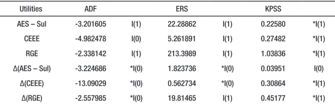
Table 1 – Unit root ADF, ERS and KPSS tests applied to the variable FEE distributed by the utilities AES-Sul, CEEE and RGE.

Utilities ADF ERS KPSS

AES – Sul -3.201605 I(1) 22.28862 I(1) 0.22580 *I(1) CEEE -4.982478 I(0) 5.261891 I(1) 0.27482 *I(1) RGE -2.338142 I(1) 213.3989 I(1) 1.03836 *I(1) ∆(AES – Sul) -3.224686 *I(0) 1.823736 *I(0) 0.03951 I(0)

∆(CEEE) -13.09029 *I(0) 0.562734 *I(0) 0.30864 *I(1) ∆(RGE) -2.557985 *I(0) 19.81465 I(1) 0.45177 *I(1)

Source: Results of the search conducted by the authors.

Notes: critical values of MacKinnon (1996): critical values for ADF test are: 1% -4.036983; 5% -3.448021; 10% -3.149135, considering the series level. Critical values for ADF test are: 1% -2.584539; 5% -1.943540; 10% -1.614941. Critical values for testing ERS are: 1% 4.192800; 5% 5.646400; 10% 6.812400, using Elliott-Rothenberg-Stock (1996). Table 1. Critical values for KPSS test are 1% 216000; 5% 0.146000 and10% 0.119000; Kwiatkowski-Phillips-Schmidt-Shin (1992). Table 1. ∆ represents the series in first difference. Values significant at 1%. 5% and 10% are represented respectively by *. **. **, indicating a rejec-tion of the hypothesis H0.

A constraint presented by the PP and KPSS tests was noted by Baillie et al. (1996). Such tests do not have the ability to detect the need for a fractional differentiation to stabilize the process. The au-thors Figueiredo & Marques (2009) stress that the PP and KPSS tests only explore the boundaries I(1) or I(0) and thus they are not able to detect the need to implement an integration of a fractional order.

From the preliminary analysis presented on the stationarity of the series, there is an impasse re-garding the order of integration. Therefore, a general ARIMA model is fitted and later a general class of ARFIMA. Thus, there is a strong indication that the company series AES-Sul can be represented by a fractional model (LI et al., 2007).

(10)

GEPROS.

Gestão da Produção,

Operações e Sistemas – Ano 6,

nº 3,

Jul-Set/2011,

p

. 23-39

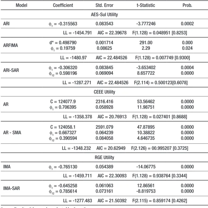
Table 2 – Models of Electrical Energy delivered to the industrial sector in Rio Grande do Sul.

Model Coefficient Std. Error t-Statistic Prob. AES-Sul Utility ARI ϕ1 = -0.315563 0.083543 -3.777246 0.0002 LL = -1454.791 AIC = 22.39678 F(1.128) = 0.048951 [0.8253] ARFIMA d* = 0.498790_ϕ 1 = 0.19759 0.001714 0.08625 291.002.29 0.0000.024 LL = -1480.97 AIC = 22.484526 F(1.128) = 0.007749 [0.9300] ARI-SAR ϕ1 = -0.306320 ϕ₁₂ = 0.598196 0.0838450.069094 -3.6534028.657722 0.00040.0000 LL = -1287.271 AIC = 22.484526 F(2.114) = 0.500123[0.6078] CEEE Utility AR _ϕC = 124077.9 1 = 0.706395 2316.416 0.058928 53.5646211.98751 0.00000.0000 LL = -1358.378 AIC = 20.76913 F(1.128) = 0.027401 [0.8688] AR - SMA ϕC = 124058.11 = 0.667327 ϕ12 = 0.390594 2591.079 0.064239 0.084058 47.87895 10.38822 4.646735 0.0000 0.0000 0.0000 LL = -1348.232 AIC = 20.62949 F(2.126) = 00.995207 [0.3725] RGE Utility IMA _ϕ₁ = -0.765130 0.054389 -14.06775 0.0000 LL = -1459.711 AIC = 22.30093 F(1.128) = 0.938764 [0.3344] IMA-SAR ϕ1 = -0.645258 ϕ12 = 0.785614 0.061063 0.073161 -8.81975312.86561 0.00000.0000 LL = -1277.483 AIC = 21.50392 F(2.115) = 0.859174 [0.4262]

Note: LL = Log likelihood, AIC = Akaike Information Criterion. The results for the ARCH-LM test using F statistics de-monstrate the exact test statistics in brackets, the null hypothesis, which indicates that there is no existence of the effects of volatility in the series.

(11)

Gestão da Produção,

Operações e Sistemas – Ano 6,

nº 3,

Jul-Set/2011,

p

. 23-39

All the residues produced by the models presented in table 2 were considered to be white noise and the Durbin-Watson statistics demonstrated a value around 2.0 for all models. The test for checking the presence of the effect of residual heteroskedasticity developed by Engle (1982), indicated the accep-tance of the null hypothesis through no autoregressive conditional heteroskedasticity (ARCH) effect in the residues, as shown in the F statistics.

Table 3 – Table of eigenvalues and the proportion of total explained variance by each utility under study.

Utilities eigenvalues % explained variance Associated forecast models

AES-Sul 2.2590320.606278 0.134689 75.30107 20.20928 4.489650 ARI ARFIMA ARI-SAR CEEE 1.976588_0.023412 98.82938_1.17062 _AR-SMAAR RGE 1.562807 0.437193 78.1403521.85965 IMA-SMAIMA

This step was used to select eigenvalues as shown by Johnson & Wichern (1992) and Hair et al. (2005). This way, it was possible to select the weights of each model in relation to the predicted com-bination. It is noted that the AES-Sul company presented three useful models for forecasting, which really constitutes a multivariate case for the application of PCA. On the other hand, the utilities CEEE, RGE presented two possible models, but even so the method was applied and validated.

Using the forecasts and eq. 19, the eigenvalues were found to calculate the total proportion of va-riance explained by each PC. This way, we have the following combinations of expressions for the FC from the forecast models (see eq. 20, 21 and 22).

(20) AES – Suli = 2.259032

3 . ARIi + 0.6062783 . ARFIRMAi + 0.1346893 . ARI – SARi

(21)

CEEEi = 1.976588

2 . ARi + 0.0234122 . AR – SMAi

(22)

RGEi = 1.562807

(12)

GEPROS.

Gestão da Produção,

Operações e Sistemas – Ano 6,

nº 3,

Jul-Set/2011,

p

. 23-39

Therefore, we obtained the weight of each model used in the forecast. The index i represents the steps envisaged for each model as the 12 steps ahead were used, utilizing i = 1, 2, ...12 etc. which cor-responds to the months from January to December 2009 (forecasts corresponding to the year 2009).

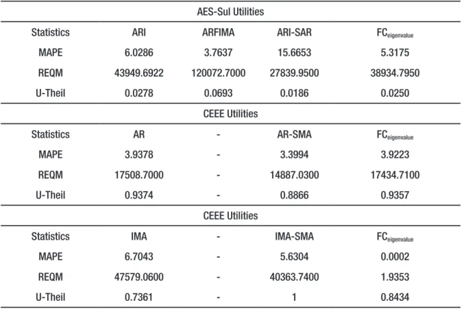
Since the purpose of this research was to verify the performance of the proposed method based on eigenvalues according to eq. 19, we used the expressions 7, 8 and 9 (table 4).

Table 4 shows that the combination of forecasts by means of FC always presents at least one result better than individual forecasting, using MAPE, REQM and U-Theil criteria. It is important to highli-ght that the FC was able to gather all the information from the individual models.

Table 4 – Representative measures of performance assessments of FC.

AES-Sul Utilities

Statistics ARI ARFIMA ARI-SAR FCeigenvalue

MAPE 6.0286 3.7637 15.6653 5.3175 REQM 43949.6922 120072.7000 27839.9500 38934.7950 U-Theil 0.0278 0.0693 0.0186 0.0250

CEEE Utilities

Statistics AR - AR-SMA FCeigenvalue

MAPE 3.9378 - 3.3994 3.9223 REQM 17508.7000 - 14887.0300 17434.7100 U-Theil 0.9374 - 0.8866 0.9357

CEEE Utilities

Statistics IMA - IMA-SMA FCeigenvalue

MAPE 6.7043 - 5.6304 0.0002 REQM 47579.0600 - 40363.7400 1.9353 U-Theil 0.7361 - 1 0.8434

Figures 1, 2 and 3 show the original values and the forecasted ones, using individual models and the FC.

(13)

Gestão da Produção,

Operações e Sistemas – Ano 6,

nº 3,

Jul-Set/2011,

p

. 23-39

Figure 1 – Comparison between the original variable AES-Sul and the values forecasted for 2009 using

the models ARI, ARI-SAR, ARFIMA and FCeigenvalue.

Figure 1 shows that the FC method reveals all movements from the individual models and rea-ches the final match for the period. The FC is explained as 75% by the ARI model.

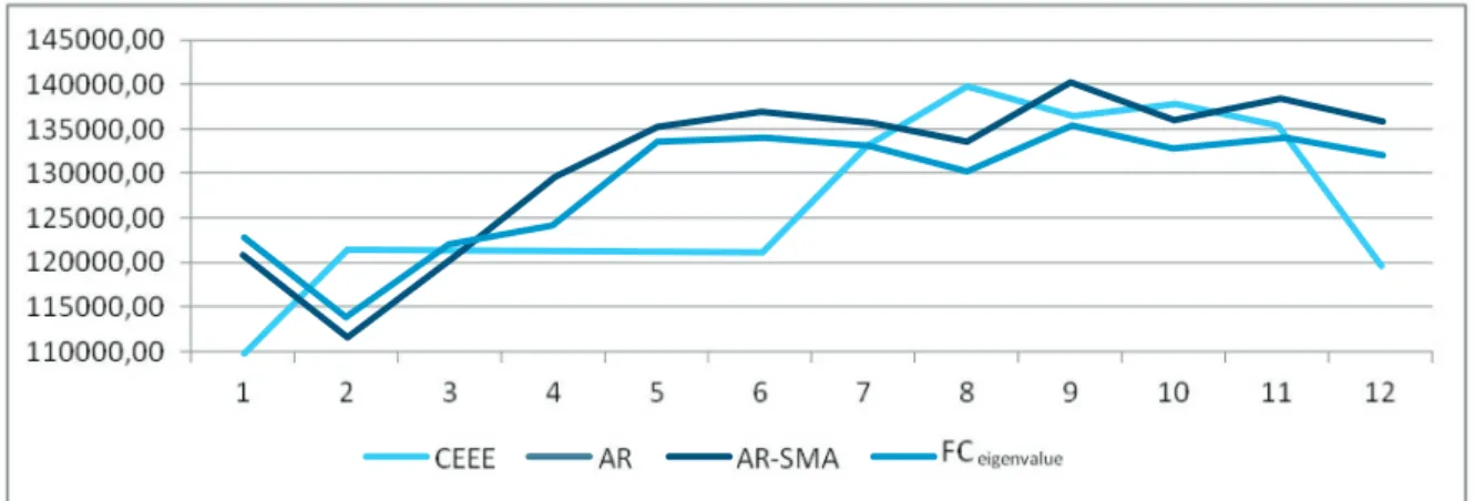
Figure 2 – Comparison between the original variable CEEE and the forecast values for 2009 by the

models AR, AR-SMA and FCeigenvalue.

Figure 2 looks as if there is a mistake because there only appear three sets of forecasting values, and the predicted values of AR models are missing. However, when analyzing the eigenvalues, one can see that 98% of the FC method is explained by the AR model, so there are overlaps of the combination method with the AR model. Even so, the proposed FC model is slightly better than the individual

(14)

fore-GEPROS.

Gestão da Produção,

Operações e Sistemas – Ano 6,

nº 3,

Jul-Set/2011,

p

. 23-39

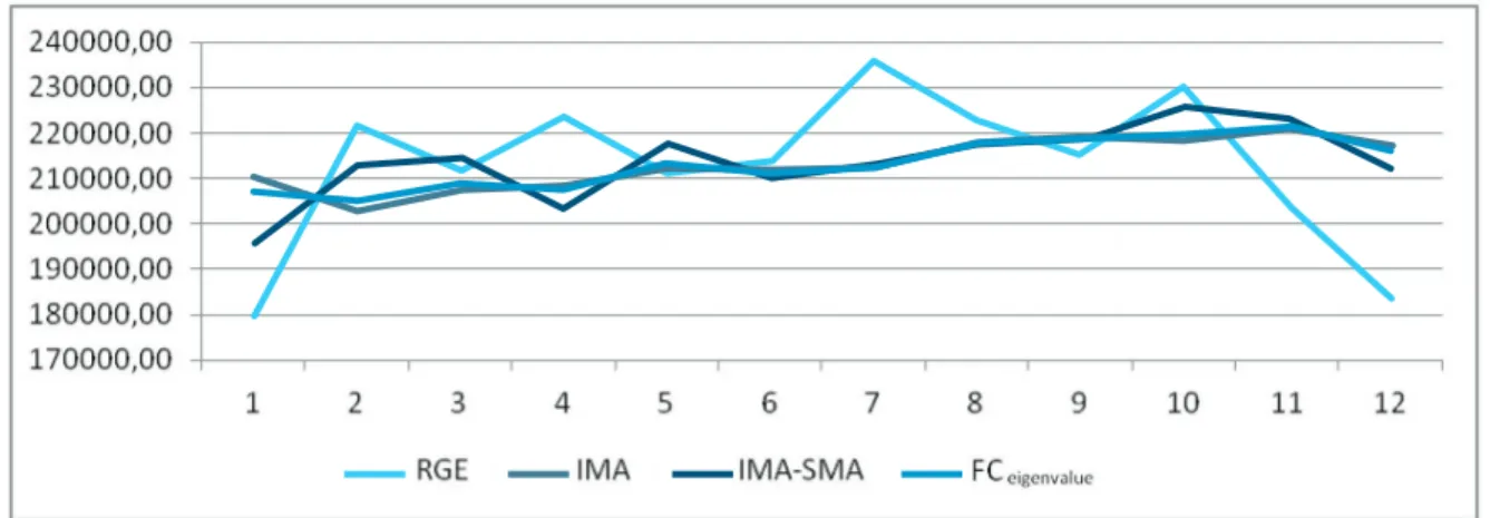
Figure 3 – Comparison among the original variable RGE and the values forecasted to 2009 by the mo-dels AR, AR-SMA and FCeigenvalue.

In figure 3 it can be observed that the FC method has become smoother than the original data, but it retains the same movements of the RGE series. The IMA model has a greater representation in the combination, responsible for 78% of explanation.

Besides bringing all the peculiarities of individual models, this model has the advantage of being a mathematical method that does not need to follow requirements such as normality and other stylized factors.

5. CONCLUSIONS

This study was able to develop a new method of FC which demonstrated a predictive capacity compatible with the techniques used for forecasting. The FC includes information and features for all models considered and not just a specific model to represent the series under study.

The technique of PCA according to Malhorta (2001) suggests that the number of observations should be at least five times higher than the number of variables, and this situation must be observed in order to not affect the performance of the proposed method.

The suggestion for further research is to include ARCH models, as well as to compare this propo-sed method with other methods of FC.

(15)

Gestão da Produção,

Operações e Sistemas – Ano 6,

nº 3,

Jul-Set/2011,

p

. 23-39

6. ACKNOWLEDGMENTS

We would like to thank CAPES Foundation for their financial support – BEX 1784/09-9 and the Ministry of Education for Brazil – Brasilia. The authors also thank the financial support provided by Fundação para a Ciência e Tecnologia (FCT) under their grants nº PTDC/GES/73418/2006 and nº PTDC/GES/70529/2006.

7. REFERENCES

AMORIM JÚNIOR, H. P; MOREIRA, T. C.; PESSANHA, V. G.; JACINTO, A. M. Previsão da demanda de passageiros no Sistema de Transporte Coletivo utilizando as Redes Neurais Artificiais e os Algorit-mos Genéticos. IV Congresso Brasileiro de Computação – CBComp, 2004.

BAILLIE, R.; CHUNG, C. F.; TIESLAU, M. A. Analyzing inflation by the fractionally integrated ARFI-MA-GARCH model. Journal of Applied Econometrics, 11: 23-40, 1996.

BATES, J. M.; GRANGER, C. W. J., The combination of forecasts. Operations Research Quarterly, 20, 319-325, 1969.

BERAN, J. Statistics for long memory processes. New York: Chapman and Hall, 1994.

BOX, G. E. P.; JENKINS, G. M. Time Series Analysis: Forecasting and Control. San Francisco: Hol-den-Day, 1970.

CLEMEN, R.T. Combining forecasts: a review and annotated bibliography. International Journal of

Forecasting. v.5, 1989.

CORRAR, J. L.; PAULO, E.; DIAS FILHO, J. M. Análise multivariada para os cursos de

administra-ção, ciências contábeis e economia. FIPECAF – Fundação Instituto de Pesquisas Contábeis, Atuariais

e Financeiras. Ed. Atlas, São Paulo, 2007.

DIEBOLD, F. X.; LOPEZ, J. A. Forecast evaluation and combination. In: NB ER Working Paper n.

T0192. Available at: http://ssrn.com/abstract=225136, Mar, 1996.

DICKEY, D. A.; FULLER W. A. Distribution of the estimators for autoregressive time series with a unit root, Journal of the American Statistical Association 74, 427-431, 1979.

ENDERS, W. Applied econometric time series. Wiley series in probability and mathematical statistics. John Wiley and Sons, Inc., New York. N.Y. 1995.

ENGLE, R. F. Autoregressive conditional heteroscedasticity with estimates of the variance of U.K. in-flation. Econometrica, v. 50, p. 987-1008, 1982.

(16)

GEPROS.

Gestão da Produção,

Operações e Sistemas – Ano 6,

nº 3,

Jul-Set/2011,

p

. 23-39

FARIAS, E. R.; ROCHA, F. J. S; LIMA, R. C. Critérios de seleção de modelos sazonais de séries

tem-porais: uma aplicação usando a taxa de desemprego da região metropolitana de Recife. III Encontro

Regional de Estudos do Trabalho – ABET, 22 a 24 de novembro de 2000 – Recife, PE. Disponível em: <http://www.race.nuca.ie.ufrj.br/abet/3reg/39.DOC>. Acesso em: 20 nov., 2005.

Economics and Statistics Foundation of Rio Grande do Sul-FEE-RS. Disponível em http://www.fee.

rs.gov.br. Acesso em: 10 maio, 2010.

FIGUEIREDO, E. A.; MARQUES, A. M. Inflação Inercial como um Processo de Longa Memória: Análise a partir de um Modelo Arfima-Figarch. Est. Econ., São Paulo, v. 39, n. 2, p. 437-458, abril-ju-nho, 2009.

GEWEKE, J.; PORTER-HUDAK, S. The estimation and application of long memory time series mo-dels. Journal of Time Series Analysis, v. 4, p. 221-238, 1983.

GRANGER, C. W. J.; JOYEUX, R. An introduction to long-memory time series models and fractional differencing. Journal of Time Series Analysis, v. 1, p. 15-29, 1980.

HAIR, J. F. JR.; ANDERSON, R. E.; TATHAM, R. L.; BLACK, W. C. Análise Multivariada de Dados. 5 ed. São Paulo: Bookmman, 2005.

HOSKING, J. R. M. Fractional differencing. Biometrika, v. 68, n. 1, p. 165 – 176, April, 1981.

HOTTELLING, H. Analysis of a complex of Statistical variables into principal components. The

Jour-nal of EducatioJour-nal Psychology, v.24, p.417 – 441/498 – 520, 1933.

JACKSON, J. E. Principal components and factor analysis: Part I – principal components. Journal of

Quality Technology, October. v.12, n.4, p. 201 – 213, 1981.

JACKSON, J. E. Principal components and factor analysis: Part II – additional topics related to princi-pal components. Journal of Quality Technology, January, v.13. n.1, p.46 – 58, 1981.

JIN, H.; FRECHETE, D. L. Fractional integration in agricultural futures proces volatilities. American

journal of Agricultural Economics, v. 86, n. 2, maio, 2004.

JOHNSON, R. A.; WICHERN, D. W. Applied multivariate statistical analysis. 3 ed. Prentice-Hall. New Jersey, 1992.

KWIATKOWSKIi, D.; PHILLIPS, P. C. B.; SCHMIDT, P.; SHIN, Y. Testing the null hypothesis of statio-narity against the alternative of a unit root, Journal of Econometrics 54, 159-178, 1992.

LI, Q.; TRICAUD, C.; SUN, R.; CHEN, Y. Q. Great salt lake surface level forecasting using figarch mo-deling. Proceedings of International Design Engineering Technical Conferences & Computers and

Information in Engineering Conference IDETC/CIE (DETC2007-34909), September 4-7, Las Vegas,

(17)

Gestão da Produção,

Operações e Sistemas – Ano 6,

nº 3,

Jul-Set/2011,

p

. 23-39

LIBBLY, R.; BLASHFIELD, R. K. Performance of a Composite as a Function of Number of Judges.

Organizational Behavior and Human Performance, v. 21, 1978.

MADDALA, G. S. Introduction to econometrics. 2. ed. Prentice-Hall Inc. Englewood Cliffs, New Jersey, 1992.

MAKRIDAKIS, S. G.; WINKLER, R. L. Averages of forecasts: some empirical results. Maganament

Science. v.29, n.9, 1983.

MALHORTA, N. K. Pesquisa de Marketing: uma orientação aplicada. 3° ed. Bookmann. Porto Alegre, 2001.

MORETTIN, P. A. Econometria financeira: um curso em séries temporais financeiras. Anais 17º Sim-pósio Nacional de Probabilidade e Estatística, ABE, Caxambu, 2006.

MORRISON, D. F. Multivariate statistical methods. 2. Ed., New York, NY. MaC Graw Hill, 1976. PAIVA, A. P. Metodologia de superfície de resposta multivariada: uma proposta de otimização para processos de soldagem com múltiplas respostas correlacionadas baseada na análise de componentes principais. Tese de Doutorado do Instituto de Engenharia Mecânica da Universidade Federal de Itaju-bá, 2006.

PEARSON, K. On lines and planes of closed fit to system of point in space. Philosophical. Magazine, v. 6, p. 559 – 572, 1901.

PHILLIPS, P. C. B.; PERRON, P. Testing for a Unit Root in Time Series Regression, Biometrika, 75, 335–346, 1988.

RAUSSER, G. C.; OLIVEIRA, R. A. An econometric analysis of wilerness area use. Journal of the

American Statical Association, v.71, n.354, 1976.

REINSEL, G. C. Elements of multivariate time series analysis. Springer-Verlag. New York, 1993. REIS, E. Estatística multivariada aplicada. Edições Sílabo, 2. Ed. 2001.

RIGÃO, M. H.; SOUZA, A. M. Identificação de variáveis fora de controle em processos produtivos multivariados. Revista Produção, v. 15, n. 1, p. 074-086, Jan./Abr. 2005.

SEBER, G. A. F. Multivariate observation. Wiley Series in Probability and Mathematical Statistics. John Wiley and Sons, Inc. NY, 1984.

WERNER, L. Um modelo Composto para realizar previsão de demanda através da integração da

Combinação de previsões e do ajuste baseado na opinião. Tese de Doutorado do Curso de

Pós-Gra-duação em Engenharia de Produção da Universidade Federal do Rio Grande do Sul, 2004. ZIVOT, E; WANG, J. Modelling financial time series with SPLUS. New York: Springer, 2003.

(18)