Low Reynolds Number Fowler Flap Design

(1)

UNIVERSIDADE DA BEIRA INTERIOR

Engenharia

Low Reynolds Number Fowler Flap Design

André da Silva Oliveira

Dissertação para obtenção do Grau de Mestre em

Engenharia Aeronáutica

(Ciclo de estudos integrado)

Orientador: Prof. Doutor Miguel Ângelo Rodrigues Silvestre

(2)

(3)

iii

Agradecimentos

Gostaria de agradecer àqueles que contribuíram não só para a realização deste trabalho, mas ao longo do curso.

Primeiramente, quero agradecer ao Professor Doutor Miguel Ângelo Rodrigues Silvestre, orientador desta dissertação, pela oportunidade de trabalhar com ele num tema que é ao mesmo tempo desafiador e interessante, e pela motivação e partilha de conhecimento prestadas que possibilitaram a conclusão desta dissertação.

Quero também agradecer à minha família pelo apoio incondicional e pela confiança depositada em mim ao longo desde percurso.

Agradeço à minha namorada, Catarina, por constantemente me ter dado confiança e motivação para continuar a olhar para o futuro com otimismo.

Por fim, quero agradecer aos meus amigos que me acompanharam ao longo destes anos pelo companheirismo e pelo apoio prestado.

(4)

(5)

v

Resumo

O Air Cargo Challenge é uma competição internacional que promove a inovação no âmbito do desenvolvimento de aeronaves não tripuladas de pequena escala, avaliando para isso as aeronaves participantes através de indicadores de performance como carga útil máxima, e limitando algumas das suas características como envergadura máxima e sistema propulsivo. Dada a participação assídua do Departamento de Ciências Aeroespaciais da Universidade da Beira Interior nesta competição, e considerando a falta de informação acerca do uso de dispositivos híper sustentadores para aplicações a baixos números de Reynolds (60,000<𝑅𝑒<500,000), um Fowler flap foi estudado com base num perfil alar previamente utilizado nesta competição. Para este processo de design do flap foram utilizados métodos de dinâmica dos fluidos computacional (CFD) através do software open-source OpenFOAM. Posteriormente, foi desenhado um protótipo de um mecanismo de atuação para a operação deste dispositivo. O flap obtido neste estudo produziu melhorias de performance consideráveis no perfil alar original, com um aumento de 𝐶𝑙_𝑚𝑎𝑥 de 1.86 para 2.96. Como seria de esperar, do

uso do Fowler flap, o momento de arfagem criado pelo perfil, 𝐶𝑚, foi intensificado, com o seu

valor a variar de -0.251 no perfil simples para -0.694 no perfil com flap. O protótipo do mecanismo de atuação desenhado neste estudo permite um movimento satisfatório durante a ativação do flap, conseguindo ao mesmo tempo manter uma dimensão compacta que o permita ser contido dentro da asa quando retraído, evitando assim perdas de performance devido ao arrasto parasita devido à incorporação do flap.

Palavras-Chave

(6)

(7)

vii

Abstract

Air Cargo Challenge is an international competition promoting innovation in the field of small scale unmanned aircraft development, evaluating the participating aircraft through performance indicators such as maximum payload, and limiting some of its characteristics such as maximum wingspan and propulsion system. Given the frequent participation of Department of Aerospace Sciences from University of Beira Interior in this competition, and considering the lack of information concerning the use of high lift devices for low Reynolds number applications (60,000<𝑅𝑒<500,000), a Fowler flap was studied based on an airfoil previously used at this competition. For this flap design process, Computational Fluid Dynamics (CFD) methods were used through the open-source software OpenFOAM. Afterwards, an actuation mechanism prototype was designed for the operation of this device. The flap obtained with this study produced significant performance improvements over the original airfoil, with an increase in 𝐶𝑙

from 1.86 to 2.96. As would be expected, from the use of a Fowler flap, the pitching coefficient created by the airfoil, 𝐶𝑚, was intensified, with its value varying from -0.251 on the clean

airfoil to -0.694 on the flapped airfoil. The actuation mechanism prototype designed in this study allowed for a satisfactory movement during the flap’s deployment, managing at the same time to maintain a compact size that allows it to be fully contained inside the wing when retracted, avoiding, in this way, any losses in performance due to parasitic drag from the incorporation of the flap.

Keywords

(8)

(9)

ix

List of Figures

Figure 2.1: Flap housing. a – NACA tests; b – RAE tests [3] ... 4

Figure 2.2: Slot parameters [4] ... 5

Figure 2.3: Fowler flap 30% chord [4] ... 11

Figure 2.4: a - Fowler flap 29% chord; b – Trailing edge detail [4] ... 11

Figure 2.5: Confluence of the two boundary layers at 50% of the flap’s chord [14] ... 13

Figure 2.6: a - standard cove; b - sharp lip cove; c - blended cove [5] ... 14

Figure 3.1: UBI_ACC11 airfoil ... 20

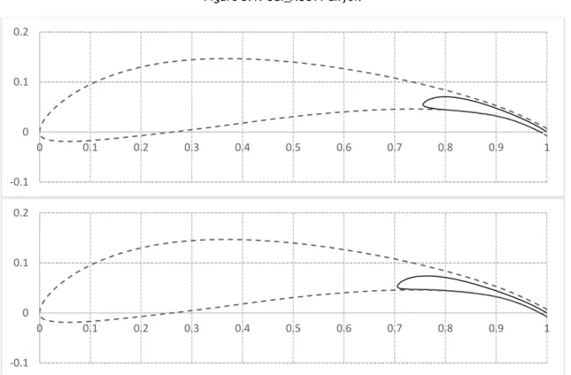
Figure 3.2: Flap airfoils: top – 25% chord flap; bottom – 30% chord flap ... 20

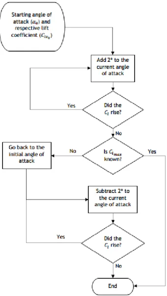
Figure 3.3: Process to determine the angles of attack to be tested... 21

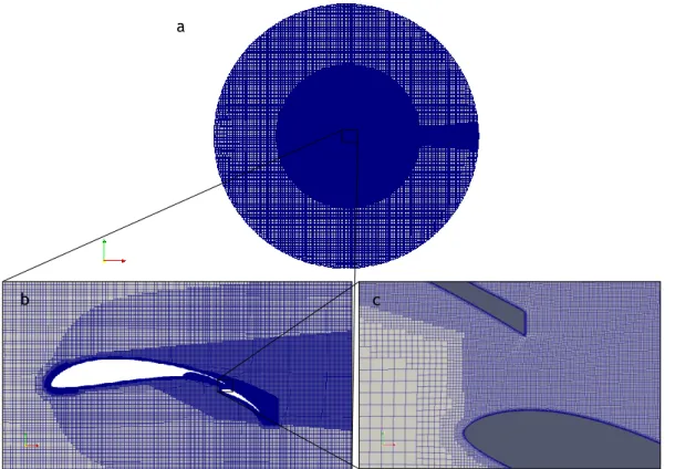
Figure 3.4: Mesh example. a – overall mesh; b – mesh near airfoil; c – wall layers detail ... 24

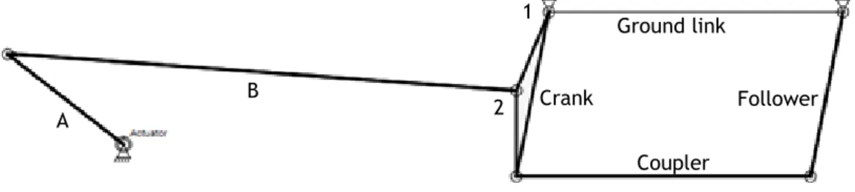
Figure 3.5: Example of a 4-bar linkage with the actuator mounted away from it ... 28

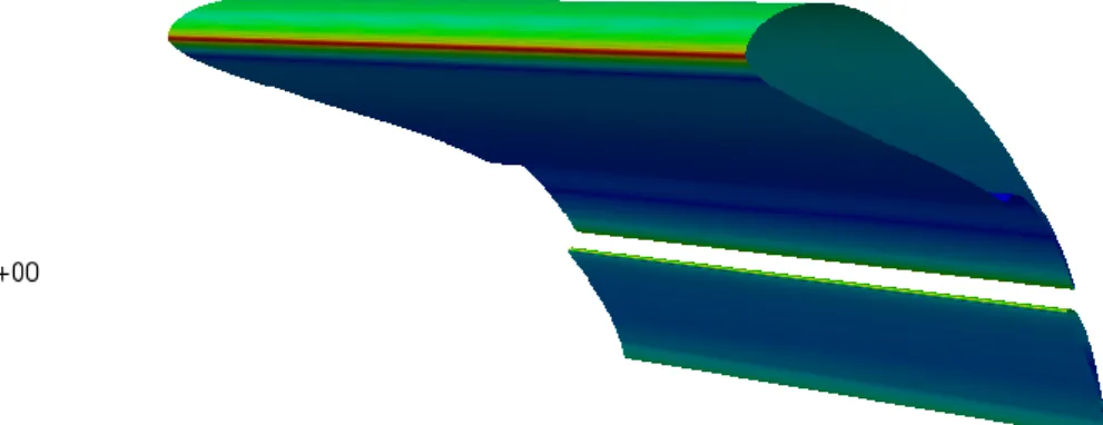
Figure 4.1: Distribution of 𝑦+_{along the surface of the wing ... 30}

Figure 4.2: Influence of mesh resolution on the aerodynamic coefficients ... 31

Figure 4.3: Selig S1223 airfoil ... 32

Figure 4.4: CFD and XFOIL comparison - 𝐶𝑙 vs 𝛼 ... 32

Figure 4.5: Result validation - 𝐶𝑙 vs 𝛼 ... 33

Figure 4.6: Result validation - 𝐶𝑙 vs 𝐶𝑑 ... 33

Figure 4.7: 25% chord Fowler flap - 𝐶𝑙 vs 𝛼 ... 35

Figure 4.8: 25% chord Fowler flap - 𝐶𝑙 vs 𝐶𝑑 ... 36

Figure 4.9: 25% chord Fowler flap - 𝐿/𝐷 vs 𝐶𝑙 ... 37

Figure 4.10: Variation of the flow patter over time at a 10° angle of attack ... 39

Figure 4.11: 30% chord Fowler flap - 𝐶𝑙 vs 𝛼 ... 40

Figure 4.12: 30% chord Fowler flap - 𝐶𝑙 vs 𝐶𝑑 ... 41

Figure 4.13: 30% chord Fowler flap - 𝐿/𝐷 vs 𝐶𝑙 ... 42

Figure 4.14: Flap comparison - 𝐶𝑙 vs 𝛼 ... 45

Figure 4.15: Flap comparison - 𝐶𝑙 vs 𝐶𝑑 ... 45

Figure 4.16: Flap comparison - 𝐿/𝐷 vs 𝐶𝑙 ... 46

Figure 4.17: Flap comparison - 𝐶𝑚 vs 𝐶𝑙 ... 46

Figure 4.18: UBI_ACC11 airfoil with no flap (𝛼=4°) ... 48

Figure 4.19: UBI_ACC11 airfoil with 2.5% gap, 2% overlap, 25% chord and 30º angle Fowler flap (α=4°) ... 48

Figure 4.20: Flow over flapped airfoil at 𝛼=0° ... 49

Figure 4.23: Flap actuation mechanism: top – flap retracted; middle – partial deployment; bottom – flap fully deployed ... 51

Figure A.1: Log generated by checkMesh ... 57

(11)

xi

List of Tables

Table 2.1: Pros and cons of each mechanism according to Peter Rudolph [24]. ... 17

Table 3.1: Flap parameters used ... 20

Table 4.1: 25% relative chord Fowler flap simulations results ... 38

(12)

xii

List of Abbreviations

ACC – Air Cargo Challenge

CFD – Computational Fluid Dynamics

NACA – National Advisory Committee for Aeronautics NASA – National Aeronautics and Space Administration PISO - Pressure Implicit with Splitting of Operators RAE – Royal Aircraft Establishment

RANS – Reynolds Averaged Navier-Stokes

SIMPLE - Semi-Implicit Method for Pressure-Linked Equations SST – Shear Stress Transport

UAV – Unmanned Aerial Vehicle UBI - University of Beira Interior

URANS – Unsteady Reynolds Averaged Navier-Stokes

(13)

xiii

List of Symbols

𝑐 – Airfoil chord 𝐶 – Courant number 𝐶𝑑 – Drag coefficient

𝐶𝐷𝑖 – Induced drag coefficient

𝐶𝑙 – Lift coefficient

𝐶_{𝑙𝑚𝑎𝑥} – Maximum lift coefficient 𝐶𝑚 – Pitching moment coefficient

𝑘 – Turbulence kinetic energy [𝑚2_/𝑠2_]

𝐿/𝐷 – Lift-to-drag ratio 𝑝 – Pressure [𝑃𝑎] 𝑅𝑒 – Reynolds number 𝑢 – Fluid velocity [𝑚/𝑠]

𝑦+_{– Dimensionless wall distance}

𝛼 – Angle of attack

𝛼𝐶𝑙𝑚𝑎𝑥 – Angle of attack for maximum lift coefficient 𝜖 – Turbulence dissipation [𝑚2_/𝑠3_]

𝜇 – Dynamic viscosity [𝑁 ∙ 𝑠/𝑚2_]

𝜈 – Kinematic viscosity [𝑚2_/𝑠]

𝜌 – Fluid density [𝑘𝑔/𝑚3_]

𝜏 – Shear stress [𝑃𝑎] 𝜏𝑤 – Wall shear stress [𝑃𝑎]

(14)

(15)

1

Chapter 1

1. Introduction

1.1. Aim and Motivation

The aim of the present study is to design a high lift system consisting of a Fowler flap for the airfoil developed for the Air Cargo Challenge 2011 competition, used by the Department of Aerospace Sciences at University of Beira Interior (UBI), through the AERO@UBI team airplane. Air Cargo Challenge (ACC) is a worldwide inter-university competition that was first held in 2003 in Portugal. The event was created by Associação Portuguesa de Aeronáutica e Espaço. This first edition of the competition required the competing teams to design and build a radio-controlled aircraft with the goal of lifting the maximum possible payload. The aircraft was required to take off within a distance of 61𝑚, complete at least one flight pattern around the airfield with the maximum payload possible, and land safely. The competition takes place every two year. From the 2007 edition, the responsibility for the organization has been EUROAVIA, the European Association of Aerospace Students together with a local EUROVIA group: normally, the winner of the last ACC edition. In all ACC editions, the competing teams have to use the same engine or motor set. Additional regulations also limited certain parameters such as wing span [1]. Throughout the years, the rules have been fine-tuned to improve the competition, with the edition, to be held in Zagreb, Croatia in 2017, taking into account both the maximum payload carried by the aircraft and the time taken to complete 10 legs in a 100 𝑚 course [2]. Due to the high level of competition in this event, it is important to ensure that the aircraft designed for the challenge makes use of any technology that may grant it a competitive edge over the other competing aircraft. Typically, the motor-propeller set mandated by the regulation offers a static thrust of about 20𝑁 and the winning airplanes are carrying 110𝑁 of payload in the form of steel ballast plates, meaning these small-scale airplanes require a lift to drag ratio, 𝐿/𝐷, well above 10 just for remaining airborne. Effectively, their (𝐿/𝐷)𝑚𝑎𝑥 is

close to 20, which is remarkable for a short take-off airplane that operates at such low Reynolds number (𝑅𝑒<500,000).

One possible way to improve the performance of an aircraft designed for this competition is to make use of high lift systems, from which the Fowler flap is known to be one of the most efficient methods for lift augmentation [3]. In the present case, a higher lift coefficient at lift-off can reduce the required airspeed thus increasing the payload while increasing the cruise lift coefficient for a better lift to drag ratio over the running course. However, there is still little research made concerning the usage of Fowler flaps for such low Reynolds number

(16)

2

(60,000<𝑅𝑒<500,000) applications, which leaves a lack of knowledge that makes the implementation of these systems harder for certain types of aircraft, most notably small UAV’s. Therefore, there was an incentive to design a Fowler flap high lift system for the airfoil used in the aircraft developed by the AERO@UBI team for Air Cargo Challenge 2011. This way, the knowledge gained from this study can be adapted to aid in the aircraft development process for the next editions of the competition, and to contribute to a better understanding of the behaviour of Fowler flaps at low Reynolds numbers.

To accomplish this goal, computational fluid dynamics techniques (CFD) were used for the design and optimization processes of the flap.

1.2. Dissertation Structure

This first introductory chapter is followed by a chapter containing the literature review which is divided into two parts: theoretical considerations, containing the theory that serves as a foundation for this project, and a second part containing the state of the art of both Fowler flap systems design and the subject of computational fluid dynamics.

The third chapter lays out the methodology used to conduct this study, being divided into the flap design process, computational simulations, and the validation of the obtained results. In the fourth chapter, the results of the study are presented and analysed.

The fifth and final chapter contains the concluding remarks for this project, as well as the recommendations for future works.

1.3. Limitations and Dependencies

The available computational power was the main limiting factor to this study. Both the mesh creation and CFD simulation tasks were performed on a laptop with 12 GB of RAM memory and a dual core processor, running at frequencies up to 1.6 GHz.

While the mesh creation software can run out of virtual memory while creating highly refined grids, causing it to abort the whole process, this was prevented by splitting the process of mesh creation into six separate tasks and running them consecutively instead of simultaneously. The usage of an O-type grid with convenient wake refinement blocks also meant that one single mesh can be used for different simulations at different angles of attack, also reducing the time spent creating meshes.

(17)

3

Chapter 2

2. Literature Review

2.1. Theoretical Considerations

2.1.1. Purpose of Flaps

A flap is a high lift device used in airplanes to enable them to alter the overall shape of the wing (mainly its curvature and effective chord), adjusting its aerodynamic performance according to the requirements of each phase of flight, obtaining an overall increase in the airplane performance. This can be done with many different types of flap, with varying complexity and effectiveness, ranging from plain flaps to flaps with multiple slots. The main types of flaps used in the trailing edge of fixed wing aircraft are [3]:

 Plain flap – consists of a portion near the trailing edge of the wing that is simply hinged;  Split flap – the trailing edge portion of the wing is split in a chordwise direction, with

the lower half being used as a flap;

 Slotted flap – when a portion of the wing near the trailing edge can rotate in such a manner that it leaves a well-defined slot between itself and the rest of the wing;  Multiple flaps – when a flap consists of more than one element, generally creating more

than one slot as well. The extra slots created my multiple flaps generally allow for a higher overall curvature.

The Fowler flap can be considered a special type of slotted flap. It not only rotates as to increase the wing’s curvature and open a slot, it also moves in the downstream direction, increasing the wing’s chord. These two effects combined make this type of flap the most effective in the present application.

To develop an optimized flap, it is necessary to identify the performance goals for each flight phase that might require the deployment of the flaps. These objectives can be summarized as follows [4]:

 Take-off: obtain a satisfactory 𝐶𝑙_𝑚𝑎𝑥 at an angle of attack that can be achieved during

rotation without provoking a tail strike;

 Climb: ensure that the point of 𝐿/𝐷𝑚𝑎𝑥 occurs for a 𝐶𝑙 equal or higher than the climb

𝐶𝑙 to prevent the aircraft from operating with reducing required power versus cruise

airspeed normally known as the reverse command region. Therefore, the priority in this phase of flight is to keep the 𝐶𝑑 as low as possible. Additionally, since the drag produced

(18)

4

at an angle of attack higher than its cruise angle, the angle of attack for which the climb 𝐶𝑙 occurs should be as close as possible from the cruise angle of attack;

 Landing: since in the approach and landing phases the aircraft is expected to operate at low speeds, the goal of the flap system here is to obtain the highest 𝐶_{𝑙𝑚𝑎𝑥} possible, with high 𝐶𝑑 values being acceptable. A reduction of the aircraft 𝐿/𝐷 during the final

glide increases the landing precision.

2.1.2. Fowler Flap Geometry

In the early wind tunnel tests on wings with Fowler flaps, there were two main ways to define the shape of the opening in the fixed element of the airfoil that would house the flap in its retracted position: in the wind tunnel tests conducted by NACA, the housing of the flap consists of a cut on the main airfoil in a right angle to its lower surface (Fig. 2.1 a); in the RAE tests, this housing was shaped in such a way that the flap would fit into the main airfoil as fairly as possible (Fig. 2.1 b) [3].

Figure 2.1: Flap housing. a – NACA tests; b – RAE tests [3]

The results of these tests reveal that between these two types of geometry, the RAE-type flap housing delivers the most favourable performance, producing a considerably lower drag coefficient as well as a slightly higher lift coefficient when compared to its NACA counterpart. Furthermore, there is no need to design a smooth shape in the region between the lower surface of the main airfoil and the housing of the flap, as seen in Figure 2.1 b. Studies have found that there is no loss in performance when opting for a cove with a sharp edge near the region that will hold the flap’s leading edge (as seen in Figure 2.6 b), as long as the airflow passing through this area has the opportunity to reattach to the main airfoil’s surface before reaching its trailing edge [5].

To find out the optimum position of the flap relative to the main airfoil, one can resort to an iterative method used by Wentz and Seetharam, in which different combinations of the slot’s gap and overlap are tested for a given flap angle [4]. The slot’s gap and overlap are defined in Figure 2.2.

(19)

5

Figure 2.2: Slot parameters [4]

2.1.3. CFD Simulations

Computational fluid dynamics consists in the “analysis of systems involving fluid flow, heat transfer and associated phenomena such as chemical reactions by means of computer-based simulation” [6].

In the book Computational Methods for Fluid Dynamics, J. Ferziger and M. Perić defined the following components as the “important ingredients of a numerical solution method” [7]:

 Mathematical Model – this is the set of partial differential or integro-differential equations and boundary conditions used for predicting the flow. An appropriate mathematical model should be chosen considering the target application, i.e., whether the flow is to be considered compressible or incompressible, viscous or inviscid, turbulent or laminar, two- or three-dimensional, etc.;

 Discretization Method – this component is the method by which the differential equations are approximated by “a system of algebraic equations for the variables at some set of discrete locations in space and time”. The main approaches to this are the finite difference, finite volume, and finite element methods, and while each type of method yields the same solution if the grid is very fine, each method is more suitable to a class of problems than others;

 Coordinate and basis vector systems – the coordinate system and basis vectors used influence the way that the conservation equations are expressed. Depending on the target flow, the coordinate system can, be cartesian, cylindrical or spherical, among others, as well as fixed or moving, while the basis in which vectors and tensors are defined can be fixed or variable, covariant or contravariant, etc. The systems used here may influence the discretization method and the grid type;

 Numerical grid – the discrete locations at which the problem will be solved need to be specified. For that, a numerical grid (often simply called mesh) is used, which consists of a discrete representation of the geometrical domain of the problem, dividing this domain into a finite number of subdomains (elements, control volumes, etc.). The most common types are the structured, block-structured, and unstructured grids;

 Finite approximations – some approximations must be made in the discretization process. In a finite difference method, these approximations are made for the derivatives at the grid points, while for a finite volume method, the method used for

Flap angle Slot overlap

(20)

6

approximating surface and volume integrals must be selected. In a finite element method, one must choose the shape functions and the weighting functions. The methods used affect the accuracy of the approximations, generally increasing the memory requirement with the accuracy. So, a compromise between simplicity, ease of implementation, accuracy and computational requirements must be made;

 Solution method – the discretization process yields a large system of non-linear algebraic equations, which must be solved by a solution algorithm. The common methods used to solve these equations use successive linearization of the equations, and the resulting linear systems are generally solved by iterative techniques. The choice of a solver depends on the grid and on the type of flow;

 Convergence criteria – these criteria define when the iterative processes of the solution algorithm will stop, influencing the efficiency and accuracy of the numerical solution method.

CFD codes are divided in three main parts: pre-processing, processing, and post-processing.

2.1.3.1. Pre-processing

The pre-processing phase requires the user to specify all the information needed to solve the problem. This includes [6]:

 Defining the problem’s geometry – in the case of external aerodynamics, special care should be taken when defining the flow domain size. A flow domain too small may be responsible for the alteration of the results due to an interference between the boundaries and the flow over the body, or there may not be enough space for the wake to develop properly;

 Discretizing the geometry into a finite number of cells – the resulting mesh should result of a compromise between solution accuracy and processing time, which means that it should neither be too coarse or too fine. There should be more points in areas of the domain where it is expected to exist large gradients of the flow properties (such as boundary layers and shear layers), and less points in areas where the flow is expected to be more uniform (such as the freestream);

 Specifying the physical and chemical phenomena that need to be modelled – in the case of external aerodynamics it is important to ensure that the effect of turbulence is properly accounted for;

 Defining the physical properties of the fluid;  Setting the boundary conditions;

Enough time should be invested in pre-processing to ensure that the problem is correctly defined and without any issues, thus avoiding any unnecessary expenditure of resources only to

(21)

7 obtain unusable results. In general, the time dedicated to defining the geometry and generating an appropriate grid accounts to about 50% of the whole time spent in a CFD study [6].

2.1.3.2. Processing

A CFD problem is solved through a solution algorithm chosen by the user. In general, these algorithms take the following steps to solve a problem [6]:

 Approximation of the unknown flow variables by means of simple functions;

 Discretization by substitution of the approximations into the governing flow equations;  Solution of the algebraic equations.

The numerical solution methods can be distinguished in four main types: finite difference, finite element, spectral methods and finite volume, the latter being the most common method for CFD applications.

The finite volume method uses as basis the conservation of the flow’s properties of interest in each cell of finite size. This way, the variation of a given variable 𝜙 associated with the flow within a finite volume can be described in terms of the balance between the various processes that tend to increase or decrease it [6], i.e., inside a given control volume, this relation can be written as per equation (2.1):

[𝑅𝑎𝑡𝑒 𝑜𝑓 𝑐ℎ𝑎𝑛𝑔𝑒 𝑜𝑓 𝜙 𝑜𝑣𝑒𝑟 𝑡𝑖𝑚𝑒] =

= [𝑁𝑒𝑡 𝑓𝑙𝑢𝑥 𝑜𝑓 𝜙 𝑑𝑢𝑒 𝑡𝑜 𝑐𝑜𝑛𝑣𝑒𝑐𝑡𝑖𝑜𝑛] + [𝑁𝑒𝑡 𝑓𝑙𝑢𝑥 𝑜𝑓 𝜙 𝑑𝑢𝑒 𝑡𝑜 𝑑𝑖𝑓𝑓𝑢𝑠𝑖𝑜𝑛] + (2.1) +[𝑁𝑒𝑡 𝑟𝑎𝑡𝑒 𝑜𝑓 𝑐𝑟𝑒𝑎𝑡𝑖𝑜𝑛 𝑜𝑓 𝜙]

This type of solution algorithms contain appropriate techniques for the treatment of these components of transport (convection and diffusion), generation and change over time for each variable of interest, generally through iterative methods [6].

The equations to be solved by the algorithm depend on the modelling approach taken, and are most commonly based on the Navier-Stokes equations.

2.1.3.2.1. Reynolds-Averaged Navier-Stokes equations

The incompressible Navier-Stokes equations in conservation form can be written as per equations (2.2) and (2.3) [8]: 𝜕𝑢𝑖 𝜕𝑥𝑖 = 0 (2.2) 𝜌𝜕𝑢𝑖 𝜕𝑡 + 𝜌 𝜕 𝜕𝑥𝑗 (𝑢𝑗𝑢𝑖) = − 𝜕𝑝 𝜕𝑥𝑖 + 𝜕 𝜕𝑥𝑗 (2𝜇𝑠𝑖𝑗) (2.3)

(22)

8 where

𝑢𝑖 corresponds to the velocity components (in a 2D problem, 𝑖 = 1, 2);

𝑥𝑖 corresponds to the spatial coordinates of the domain;

𝑡 is the time variable; 𝜌 is the density of the fluid; 𝜇 is the fluid’s dynamic viscosity;

𝑠𝑖𝑗 is the strain-rate tensor, given by equation (2.4):

𝑠𝑖𝑗 = 1 2( 𝜕𝑢𝑖 𝜕𝑥𝑗 +𝜕𝑢𝑗 𝜕𝑥𝑖 ) (2.4)

In turbulent flows, the field variables 𝑢𝑖 and 𝑝 are expressed as the sum of mean and fluctuating

components:

𝑢𝑖= 𝑈𝑖+ 𝑢𝑖′ (2.5)

𝑝 = 𝑃 + 𝑝′ _(2.6)

The time averages of these components are defined to satisfy the equations (2.7) through (2.10)

𝑢̅ = 𝑈𝑖 𝑖 (2.7)

𝑢̅ = 0 𝑖′ (2.8)

𝑝̅ = 𝑃 (2.9)

𝑝_{̅ = 0}′ _(2.10)

By applying these definitions to the Navier-Stokes equations of equations (2.2) and (2.3), the result is the Reynolds-averaged Navier-Stokes (RANS) equations:

𝜕𝑈𝑖 𝜕𝑥𝑖 = 0 (2.11) 𝜌𝜕𝑈𝑖 𝜕𝑡 + 𝜌 𝜕 𝜕𝑥𝑗 (𝑈𝑖𝑈𝑗) = − 𝜕𝑃 𝜕𝑥𝑖 + 𝜕 𝜕𝑥𝑗 (2𝜇𝑆𝑖𝑗− 𝜌𝑢̅̅̅̅̅̅) 𝑖′𝑢𝑗′ (2.12)

where 𝑆𝑖𝑗 is the mean strain-rate tensor, given by equation (2.13):

𝑆𝑖𝑗 = 1 2( 𝜕𝑈𝑖 𝜕𝑥𝑗 +𝜕𝑈𝑗 𝜕𝑥𝑖 ) (2.13)

(23)

9 By applying the definition of the Reynolds stress tensor, 𝜏𝑖𝑗 = −𝑢̅̅̅̅̅̅, equation (2.12) can be 𝑖′𝑢𝑗′

expressed as follows: 𝜕𝑈𝑖 𝜕𝑡 + 𝑈𝑗 𝜕𝑈𝑖 𝜕𝑥𝑗 = −𝜕𝑃 𝜕𝑥𝑖 + 𝜈 𝜕 2_𝑈 𝑖 𝜕𝑥𝑗𝜕𝑥𝑖 −𝜕𝑢𝑖 ′_𝑢 𝑗′ ̅̅̅̅̅̅ 𝜕𝑥𝑗 (2.14)

In a turbulent flow, the Reynolds-averaged Navier-Stokes equations by themselves are a system of equations with more unknown variables than equations. To solve the problem, additional equations are taken into account in the form of turbulence models.

2.1.3.2.2. Turbulence Models

The most common turbulence models used to complete the RANS formulation are the following [9]:

 Standard 𝑘-𝜖 model – the transport equations are solved for two scalar properties of turbulence (turbulent kinetic energy, 𝑘, and its dissipation rate, 𝜖). Adequate for free-shear-layer flows with relatively small pressure gradients. Less accurate for large adverse pressure gradients in wall bounded flows;

 Standard 𝑘-𝜔 model – the convective transport equations are solved for two scalar properties of turbulence (turbulent kinetic energy, 𝑘, and its specific dissipation rate, 𝜔). Has a superior numerical stability when compared to the 𝑘-𝜖 model, and has good agreement with experimental results for mild adverse pressure gradient flows. Due to its high sensitivity to small freestream values of 𝜔, this model is not adequate for free-shear layer and adverse pressure gradient boundary flows in complex computations;  𝑘-𝜔 SST – the 𝑘-𝜔 and 𝑘-𝜖 models are blended together in a 𝑘-𝜔 formulation in order

to combine the desirable characteristics of both models into one, using the standard 𝑘-𝜔 model near solid walls and the standard 𝑘-𝜖 model near boundary layer edges and in free-shear layers. Thus, this model has an improved capability to correctly predict the behaviour of flows with strong adverse pressure gradients and separation;

 Spalart-Allmaras model – this model uses one transport equation for the turbulent viscosity. It provides smooth laminar-turbulent transition capabilities, provided that the location where the transition starts is given beforehand. This model is not adequate for jet flows, but gives reasonably good predictions of 2D mixing layers, wake flows, and flat-plate boundary layers. It also provides better results for flows with adverse pressure gradients when compared to the standard 𝑘-𝜖 and 𝑘-𝜔 models, although it is still inferior when compared to the 𝑘-𝜔 SST model.

2.1.3.3. Post-processing

The post-processing consists in the organization and analysis of the data obtained as the result of the processing phase, with the use of tables and graphs for a detailed analysis of the information, or via the representation of the flow variables throughout the domain with

(24)

10

visualization tools such as colour maps and streamlines for a quicker overview of the obtained solution.

2.1.3.4. Result Validation

There are two important steps that should be taken to ensure the validity of the obtained results: the verification and validation of the computational model [10].

The verification of the computational model consists in verifying whether it is correctly implemented, i.e., the intention is to identify and reduce the errors resulting from such factors as mesh dependence. One way to verify the model is through a benchmark test, by comparing it with an existing computational model with established high precision.

The validation consists in checking whether the computational model is representative enough of the physical problem. To validate a model, one can compare the results obtained in the CFD simulations with experimental results.

2.2. State of the Art

2.2.1. Fowler Flap

In 1932 a study was made concerning the positioning of a Fowler flap with 40% of the cord of the wing it was used on, in NACA’s 7 ft. by 10 ft. wind tunnel [11]. The wing had a chord of 0.25𝑚 with a span of 1.52𝑚 was based on the airfoil Clark Y and the tests were made with a Reynolds number of 609,000. With this study a 𝐶𝐿𝑚𝑎𝑥 of 3.17 was obtained for a flap angle of 40°, an increase of approximately 250% when compared to the basic wing without flap, which had a 𝐶_{𝐿𝑚𝑎𝑥} of 1.27. With these results an observation was made that by applying a Fowler flap to a monoplane with a parasol type wing, and neglecting the increase in weight, in order to maintain the landing speed this new wing with the Fowler flap would only need 40% of the original wing’s area.

In 1941, in a NACA report with the objective of studying the possible configurations of a slot-lip aileron in a wing with different types of flaps, it was estimated that a combination of a Fowler flap with an angle of 40° and a modified slotted flap with an angle of 35° would produce a 𝐶𝐿_𝑚𝑎𝑥 14% greater than that of a wing with a simple slotted flap [12].

At Wichita State University, in the year 1974, a Fowler flap system was developed to be used in a high performance general aviation airfoil [4]. The GA(W)-1 airfoil was used for this study with two different flaps with different relative chords, corresponding to 29% and 30% of the main chord, for Reynolds numbers ranging from 2.2×106_{and 2.9×10}6_{. For each of the flaps a} series of combinations of gap and overlap were tested, with flap angles ranging from 0° to 40° in increments of 5°, and including 50° and 60° angles as well. In this study, the airfoil with a

(25)

11 30% chord Fowler flap reached a 𝐶_{𝑙𝑚𝑎𝑥} of 3.8 with a flap angle of 40°, with gap and overlap corresponding to 2.7% and -0.7% of the main chord, respectively.

From these results, some important observations can be made: by increasing the flap angle from 35° to 40°, there is little variation in terms of 𝐶_𝑙, 𝐶_𝑑 and 𝐶_𝑚. Meanwhile, by increasing the angle from 40° to 50° there is a considerable increase of 𝐶_𝑑 with little change to 𝐶_𝑙 and 𝐶_𝑚, and a further increase in flap angle to 60° results in a severe loss of 𝐶_𝑙, as well as a large increase of 𝐶_𝑑. Furthermore, it was observed that any attempt to modify the trailing edge of the main airfoil to give it a straighter shape on its lower surface resulted in severe penalties to the airfoil’s performance.

The two flaps used in this study had a different way of fitting into the main airfoil. With the 29% chord flap, the main airfoil was design in a way so that when the flap was retracted, the last 4% of the wing’s trailing edge was comprised of the flap, or in other words, without the flap, the main airfoil only has 96% of the original chord (Figure 2.4). Meanwhile, for the 30% chord flap, the main airfoil has a complete upper surface all the way to the trailing edge, which means that the flap is completely docked in the main airfoil’s lower surface. That means that without the flap, the main airfoil remains with 100% of the original chord (Figure 2.3).

Figure 2.3: Fowler flap 30% chord [4]

Figure 2.4: a - Fowler flap 29% chord; b – Trailing edge detail [4]

a

(26)

12

With the results of the study it was concluded that the difference between the two flaps in terms of (𝐿/𝐷) _𝑚𝑎𝑥 is virtually non-existent, while in terms of 𝐶_{𝑙𝑚𝑎𝑥} the airfoil with the 30% chord flap comes out slightly on top of the 29% chord one, which is to be expected since the former ends up with a slightly larger effective chord with the flap extended. However, according to the authors, this difference in 𝐶_{𝑙𝑚𝑎𝑥} is not noticeable enough to justify the preference for this flap, but, from a structural point of view, the airfoil with the 30% chord Fowler flap ends up having a simpler manufacturing because of the finite trailing edge on the fixed component of the airfoil, unlike the trailing edge of its counterpart.

Also at Wichita State University, in 1976, a wind tunnel study was made on a wing with the GA (W)-2 airfoil with aileron, slotted flap, Fowler flap and slot-lip spoiler configurations [13]. The Fowler flap had 30% of the main airfoil’s chord, and was developed similarly to the flap used with the GA (W)-1 airfoil from reference [4]. A 𝐶_{𝑙𝑚𝑎𝑥} of 3.82 was obtained for a flap angle of 40°, and it was observed that for any flap angle, the highest values of 𝐶_{𝑙𝑚𝑎𝑥} correspond to an overlap of approximately 0%, while the optimal gap values lie between 2% and 3% of the main chord. Additionally, the authors considered it to be relevant to study optimal gap and overlap configurations for intermediate flap angles, namely 10° and 20°.

The effectiveness of each flap in terms of increase in 𝐶𝑙 for zero angle of attack and increase

of 𝐶_{𝑙𝑚𝑎𝑥} were compared. The three types of flap used in this comparison were the simple flap, single slotted flap and Fowler flap, and the effectiveness increased with complexity, meaning that the slotted flap is more effective than the simple flap, and the Fowler flap is the most effective of the three.

Still at Wichita State University, in 1977, a study was made about the flow separation on the GA (W)-1 airfoil with the 30% chord Fowler flap developed in 1974 in the same institution [4], [14]. The study was carried out with a flap angle of 40°, for angles of attack of 2.7°, 7.7° and 12.8°, with a Reynolds number of 2.2×106_{and a Mach number of 0.13.}

The three angles of attack chosen correspond to three different types of flow that can occur with this specific configuration:

 For low angles of attack (𝛼 ≤ 2.7°) there is a small zone on the flap’s trailing edge where flow separation occurs;

 This separation decreases with an increase of the angle of attack and the flow is completely attached at an angle of attack of 7.7°. With further increase of the angle of attack, flow separation starts to appear again, progressing towards the leading edge of the main airfoil;

(27)

13  At angles of attack past the stall angle (𝛼 ≥ 12.8°) the area of flow separation continues to move towards the leading edge of the main airfoil while the flow over the surface of the flap remains attached.

The results of this study suggest that for an optimal gap size, the main airfoil lower surface’s boundary layer and the flap upper surface’s boundary layer at the slot exit are separated by a finite width core flow of constant energy. This core flow disappears close to the region of the flap corresponding to half of its chord, where there is a confluence of the two boundary layers (Figure 2.5).

Figure 2.5: Confluence of the two boundary layers at 50% of the flap’s chord [14]

In 1983, again at Wichita State University, additional studies were made on the 30% chord Fowler flap for the GA (W)-1 airfoil, already subject of various studies mentioned earlier [4], [14], [15]. This time the focus of the study were the effects of changes in the flap’s overlap and gap as well as changes in the shape of the main airfoil cove used to dock the retracted flap, for a flap angle fixed at 35° [5]. To evaluate the influence of these parameters the tests were conducted for three different angles of attack – the stall angle and pre-stall and post-stall angles.

Regarding the gap, it was concluded that for optimal gap sizes (3% of the main chord) and below (2% of the main cord) the flow is similar, with the difference that for a gap smaller that the optimal size there is a larger high turbulence region with intermittent flow reversal at angles of attack equal or higher than the stall angle, resulting in a slightly lower 𝐶_{𝑙𝑚𝑎𝑥} as well. For a gap size greater that the optimal gap (5% of the main chord) there are flow separation regions on the surface of the flap for every angle of attack tested, producing rather inferior lift than the remaining configurations at angles of attack equal and lower that the stall angle.

(28)

14

In respect to the cove shape, three distinct geometries were tested, the standard cove originally developed in 1975, a sharp lip cove, consisting of the shape of the flap airfoil cut into the main airfoil, and a blended cove, a combination of the standard and sharp lip geometries (Figure 2.6).

Figure 2.6: a - standard cove; b - sharp lip cove; c - blended cove [5]

From these studies, it was concluded that with the standard and sharp lip coves there was a flow separation region at the beginning of the cove, followed by reattachment of the flow. With the blended cove, flow separation does not take place in this region. However, despite these differences, all the cove shapes produced similar velocity profiles at the exit of the gap, showing that the occurrence of separation in the cove does not negatively affect the airfoil’s 𝐶𝑙𝑚𝑎𝑥, as long as there is reattachment of the flow before it reaches the airfoil’s trailing edge. In a NASA report from 1996, Peter Rudolph listed some of the typical parameters of high lift devices used in general aviation aircraft [16]. According to the author, when it comes to single slotted flaps, the chord of the flap is usually between 20% and 35% of the main chord, and they operate with flap angles ranging from 30° to 40°, and with a gap size of approximately 2% of the main chord. The author also indicates that typical overlap values correspond to about half of the flap’s chord, although this estimate is subject to greater uncertainty.

In 2013, at Manipal Institute of Technology, a CFD study was made to evaluate various configurations of high lift systems for a wing with a NACA 2412 airfoil operating at a low Reynolds number (2×105_{), to be used in a micro air vehicle [17]. The high lift devices used in}

this study consisted of a leading edge slat and a trailing edge double slotted flap, with flap angle of 40° and angles of attack ranging from 4° to 54°. The results of this study showed that for every angle of attack tested, the gap size that produced the highest 𝐶𝑙 corresponded to

1.7% of the main chord of the wing. a

c b

(29)

15 At the Technical University of Sofia, in 2015, a study was conducted concerning the influence of a simple flap’s gap size in the aerodynamic characteristics of a NACA 23012 airfoil, with a Reynolds number of 3×106_{[18]. Two gap sizes were tested: 5% and 15% of the main airfoil’s}

chord. Various CFD simulations were made for angles of attack between 0° and 20°, concluding that the gap size has little influence on 𝐶𝑙 and 𝐶𝑑 for angles of attack lower than 16°. At this

angle of attack the airfoil hits its 𝐶𝑙_𝑚𝑎𝑥, which is higher with the wider gap. For angles of attack

lower to 16° the 𝐶𝑙 decreases on both cases, maintaining higher values with the narrower gap.

Additionally, for angles of attack of 16° and higher, the airfoil with a 15% gap always produces a lower 𝐶𝑑 than its counterpart.

2.2.2. CFD Simulations

In 1992 at NASA, Florian R. Menter presented the two-equation turbulence model 𝑘-𝜔 SST (Shear Stress Transport) which was designed to produce results comparable to the existing 𝑘-𝜔 model developed by Wilcox in 1988 [19], without its strong dependence on freestream values [20]. For this, the model is identical to the 𝑘-𝜔 model in the inner 50% of the boundary layer and gradually changes to the 𝑘-𝜖 model towards the boundary layer edge, with the additional ability to account for the transport of the principal shear stress in boundary layers with adverse pressure gradients. It was shown that the results obtained with the 𝑘-𝜔 SST model are in fact independent from the freestream values and agree with experimental data for flows with adverse pressure gradient boundary layers. The usage of a 𝑘-𝜔 formulation in the inner part of the boundary layer also gives the 𝑘-𝜔 SST model the capability to be used in low Reynolds number flows without the addition of damping functions, unlike the standard 𝑘-𝜖 turbulence model.

A study was made in 2006 at the Technical University of Braunschweig as to validate computational simulations of laminar separation bubbles on a low Reynolds number airfoil [21]. The simulations were modelled with the Reynolds-averaged Navier Stokes (RANS) equations, and at a Reynolds number of 6×104_{good agreement was found with experimental and XFOIL}

results. At certain angles of attack, it was impossible to obtain convergence of the results using the steady RANS solver, so the simulations were made in a time-accurate mode to obtain a periodic solution.

In 2013, at Delft University of Technology, CFD simulations were made of an air flow over a NACA 63-618 airfoil, used in the blades of wind turbines, by using the software OpenFOAM, with the solution algorithm simpleFoam and using the k-𝜔 SST turbulence model. This study demonstrated that the values of 𝐶𝑙 agree with experimental results up to an angle of attack of

10°, although the values of 𝐶𝑑 obtained were quite higher than experimental values, even at

zero angle of attack [22]. For these simulations two different C-type meshes were used for low Reynolds and high Reynolds simulations.

(30)

16

For the low Reynolds simulations, special care was taken to ensure that the nondimensional wall distance, 𝑦+_{, was small enough (in this case smaller than 1) to correctly simulate the}

boundary layer over the whole airfoil. Additionally, mesh independency was demonstrated by evaluating the relation between the number of nodes in the mesh and the 𝐶𝑑 obtained for the

angle of attack of 5°, i.e., the results can be considered mesh independent when a significant increase in number of nodes does not result in a significant variation in the results obtained. In 2016, at the Universidade da Beira Interior, a study was conducted to compare the precision of the XFOIL software and CFD methods for predicting the aerodynamic characteristics of high lift low Reynolds number airfoils [23]. It was demonstrated that both XFOIL and the CFD software used (in this case both ANSYS Fluent and OpenFOAM were used, with a modified 𝑘-𝑘𝑙-𝜔 model and 𝑘-𝑘-𝑘𝑙-𝜔 SST) are suitable to this purpose. For the CFD part of this study a O-type mesh was used, with the outer boundaries placed at 30 chords of distance from the airfoil, with special care taken to keep a value of 𝑦+_{lower than 1 over the whole surface of the airfoil to}

ensure that the boundary layer is properly discretized.

2.2.3. Actuation Mechanism

For an airplane to make use of a flap system, a mechanism is necessary to enable the flap to be fixated on a retracted position, docked into the main element of the wing, and to be deployed into at least one other position defined during the aerodynamic study, defined in terms of flap angle, overlap and gap. One of the factors that can be used to evaluate the performance of an actuation mechanism is the Fowler motion it provides to the flap. For a trailing edge flap, according to Peter Rudolph, this motion is “measured in linear increments in the chord plane of the respective upstream element” [16].

In a 1996 NASA report, the flap mechanisms used on commercial subsonic airliners were classified in 7 types [16]:

 Simple hinge;

 Upright, four-bar linkage;  Upside-down, four-bar linkage;

 Upside-down/upright four-bar linkage;  Complex four-bar linkages;

 Hooked-track supports;  Link/track mechanisms.

In 1998 several of these types of mechanisms were tested and evaluated according to their potential to be used in high lift devices for high aspect ratio swept wings [24]. A total of 9 different mechanisms were compared, with their pros and cons summarized in Table 2.1.

(31)

17

Table 2.1: Pros and cons of each mechanism according to Peter Rudolph [24].

Mechanism Pros Cons

Simple Hinge -

 Low Fowler motion;

 Hard to obtain a gap between the

flap and the main part of the wing. Boeing 777 Type Upside Down/Upright Four Bar Linkage -

 Mediocre Fowler motion for

typical takeoff flap angles;

 Complex;

 Deep and wide fairing

YC15 Type Upside Down Four Bar Linkage

-

 Low Fowler motion;

 High weight;

 High actuation loads;

 Deep fairing

Short Brothers Type Upside Down Four Bar Linkage

-

 Mediocre Fowler motion;

 High complexity and weight;

 Deep and long fairing

Boeing 747 SP Type Upside Down Four Bar Linkage

 Very simple;

 Rather high Fowler motion for

flap angles above 10°;

 Reasonable actuation loads;

 Small fairing - Airbus A330/340 Type Link/Track Mechanism

 Rather high Fowler motion for

takeoff flap angles;

 Reasonable actuation loads

 Deep and long fairing

Airbus A320 Type Link/Track Mechanism

 Similar to the Airbus A330/A340

mechanism, with superior Fowler motion, lower actuation loads and smaller fairing

-

Boeing Link/Track Mechanism

 Superior to the Airbus A320

mechanism in terms of Fowler motion and fairing compactness

 High actuation loads

Boeing 767 Hinged Beam Four Bar Linkage

 Good Fowler motion for small

flap angles;

 Shallow fairing

 High complexity;

 High actuation loads;

(32)

(33)

19

Chapter 3

3. Methodology

The methodology used in this study can be broken down into three separate components: the design process of the flap, the CFD simulation and the actuation mechanism design.

3.1. Flap design

When defining the airfoil shape to be used on the flap element, one must keep in mind that its lower surface will be limited to that of the wing’s airfoil lower surface, and its thickness will be limited by the trailing edge region thickness. This is because the wing must retain its original shape when the flap is retracted to avoid losses in performance, and the portion of the main airfoil’s trailing edge that sits on top of the retracted flap must have a reasonable amount of thickness that allows the wing to be built without compromising its structural integrity. The design process of the flap’s airfoil was started by the drawing of an initial shape that will serve as a basis for the final airfoil. This initial shape was optimized for its estimated operational Reynolds number (calculated as a fraction of the main airfoil’s Reynolds number, according to the flap’s relative chord) by controlling the flow’s transition points on both the lower and upper surfaces [25] using XFOIL’s inverse design capabilities [26]. The main optimization goal in this process are a high 𝐶𝑙𝑚𝑎𝑥 and a smooth lift curve in the stall region, meaning that the stall separation starts in the trailing edge progressing towards the leading edge.

With a defined flap airfoil shape, several flap configurations in terms of angle, gap and overlap must be tested with CFD for a range of angles of attack to identify the influence of those parameters in the flap’s performance. To evaluate the influence of the flap’s relative chord on its performance, the flap airfoil design process must be repeated for all different relative chords that will be evaluated before the CFD study can be done.

Based on the knowledge gathered and summarized in Chapter 2 concerning the typical optimal configurations of Fowler flaps, a starting point for this Fowler iterative process was defined. In this case, a flap with a chord equivalent to 25% of the main airfoil’s chord, a gap of 3%, overlap of 1% and a flap angle of 35° was set as the starting point.

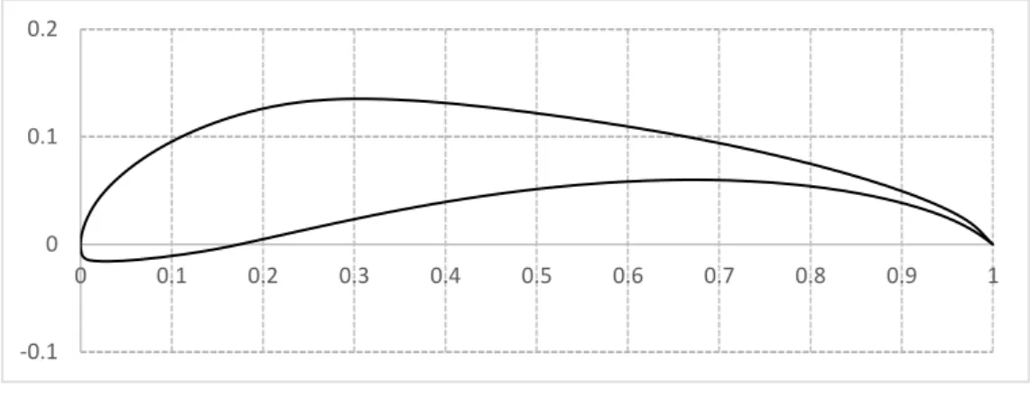
To study the influence of the Fowler flap parameters in its performance, two flaps were developed for the low Reynolds airfoil UBI_ACC11, used in previous editions of Air Cargo Challenge by the AERO@UBI team (Fig 3.1), with two different chords – 25% and 30% of the main airfoil’s chord. The airfoils developed for these flaps are presented in Figure 3.2.

(34)

20

Figure 3.1: UBI_ACC11 airfoil

Figure 3.2: Flap airfoils: top – 25% chord flap; bottom – 30% chord flap

The flap parameters tested in the CFD simulations consisted of combinations of the values of gap, overlap and flap angle listed on Table 3.1:

Table 3.1: Flap parameters used

Minimum value Maximum value

Gap 0.025𝑐 0.03𝑐 Overlap 0.01𝑐 0.02𝑐 Flap angle 30° 35° Flap chord 0.25𝑐 0.30𝑐 -0.1 0 0.1 0.2 0 0.1 0.2 0.3 0.4 0.5 0.6 0.7 0.8 0.9 1 -0.1 0 0.1 0.2 0 0.1 0.2 0.3 0.4 0.5 0.6 0.7 0.8 0.9 1 -0.1 0 0.1 0.2 0 0.1 0.2 0.3 0.4 0.5 0.6 0.7 0.8 0.9 1

(35)

21 The simulations were made in two phases: in the first series of CFD simulations, all the combinations of parameters are tested for a narrow range of angles of attack in search of the design maximum lift coefficient. Limiting these simulations to a narrow range of angles of attack is useful to minimize the overall number of simulations. The angles of attack tested for a given flap configuration were generally determined in the following manner (see Fig. 3.3): an angle of attack was chosen as a starting point, and the aerodynamic coefficients were determined at that angle. For the next simulation, the angle of attack is raised by 2°. If the 𝐶𝑙

is higher than the one obtained on the previous simulation, the angle of attack is again raised by 2°, and the process repeated until the 𝐶𝑙 value starts decreasing, determining in this way

the 𝐶_{𝑙𝑚𝑎𝑥} of the flap configuration and the approximate angle of attack in which it occurs. If, on the other hand, the 𝐶𝑙 lowers when the angle of attack is raised for the first time, the next

angle to be tested is 2° below the starting angle of attack, repeating this process until the 𝐶_{𝑙𝑚𝑎𝑥} and the approximate angle of attack at which it occurs can be determined.

(36)

22

From the results of the first series of CFD simulations, the best performing flap configurations are selected for further analysis with another series of simulations. In this second phase, the flapped airfoils are tested for a wider range of angles of attack to obtain detailed information about the performance of each flap configuration, enabling the final flap design to be determined.

3.2. CFD Simulations

All the main pre-processing, processing and post-processing tasks were made using the open-source software OpenFOAM, with each single simulation corresponding to a specific angle of attack and a specific flap configuration. A Reynolds number of 2.0×105_{corresponding to the} retracted wing chord was used for the calculations.

3.2.1. Pre-processing

For each flap configuration, the corresponding mesh was created with the use of the tools provided by the OpenFOAM package. The mesh creation process can be organized into three different phases.

On the first phase, blockMesh was used to create a base grid made up of a single uniform block of cubic cells from which the final mesh will be shaped from. When creating this grid, the size of the elements was chosen according to the desired size of the far-field cells of the final mesh, and the block itself was made to have an appropriate height to avoid the effects of blockage with the wing in it, and a length large enough to allow the wake to fully develop. Previous CFD studies have shown that for simulations concerning low Reynolds number flows over airfoils, as in this case, a distance of 30 chords between the airfoil and the outer boundaries of the computational domain is enough to produce good results [23].

On the second phase, snappyHexMesh was used to shape the base grid. By inserting 3D models of the wing with a deployed flap, its shape was cut into the existing uniform block mesh and the cells closest to the wing were refined to a smaller size. The outer boundaries of the domain were also cut from the remaining mesh using a previously prepared 3D body, in such a way as to obtain an O-type mesh. This type of mesh has great versatility since the angle of attack of the flow can be adjusted by simply changing the velocity components of the flow at the inlet. Additional 3D bodies are then used to refine the cells in regions where gradients of the flow’s properties are expected, e.g., regions with shear layers, the wake region, as well as the leading and trailing edge of both the main element of the wing and the flap. In this phase the mesh was refined enough to capture the important physical phenomena associated with the flow, but at the same time, care was taken to avoid creating a mesh that is too fine, which would greatly increase the necessary computational resources.

(37)

23 With the refinement levels properly defined, one can give use to one of the most useful features of snappyHexMesh: layer addition. By adding expanding layers to the proximity of a surface, this tool allows the addition of very fine cells adjacent to the surfaces of the wing [27], which helps to properly discretize the flow’s boundary layers. To determine if the mesh near a wall is properly defined, the parameter 𝑦+_{is used, which is the nondimensional distance that results}

from a relation between the height of the first cell adjacent to a wall and the shear velocity of the flow in that area. This parameter is calculated through the law of the wall [6], as per equation (3.1):

𝑦+₌𝜌 ∙ 𝑢𝜏∙ 𝑦

𝜇 (3.1)

where

𝑦 is the height of the first cell adjacent to the wall,

𝑢𝜏 is the shear velocity of the flow, given by equation (3.2):

𝑢𝜏= √

𝜏𝑤

𝜌 (3.2)

with 𝜏𝑤 being the shear stress on the wall.

The recommended value of 𝑦+_{depends on the turbulence model that is used in the CFD}

simulation. The decision was made to opt for a two-equation turbulence model due to the typical availability and ease of use this type of model. From this type of turbulence formulation, the Menter’s 𝑘-𝜔 SST turbulence model was used due to its independence from free-stream turbulence properties and the lack of need for any extra damping functions for it to be used with low Reynolds number flows [20]. This specific turbulence model calls for a 𝑦+_{lower than}

1 on the walls [9].

During the second phase of the mesh creation, each time a cell is refined by one level, it gets divided into four smaller cells [27]. This means that if the starting base mesh has the thickness of one element, when applying refinements with snappyHexMesh the result will be a mesh with more than one element in the direction of the span of the wing. Since the mesh is intended to be used for a two-dimensional flow, these extra elements in the third direction are unnecessary and will result in a waste of computational resources during processing. To avoid this waste, a third phase is added to the mesh creation process, where one of the faces of the mesh obtained in the second phase is extruded into a one element thick grid with 1𝑚 width, by using

extrudeMesh, a tool included in the OpenFOAM package.

(38)

24

Figure 3.4: Mesh example. a – overall mesh; b – mesh near airfoil; c – wall layers detail

With the mesh defined, OpenFOAM’s utility checkMesh was used to check if problems such as highly skewed, non-orthogonal or negative volume cells are impairing the quality of the mesh. If no problems were found, the boundary conditions were defined in the following manner [6], [28]:

 Inlet – all the variables are specified as uniform values, except for pressure, which is defined with zero gradient. The angle of attack was defined in this boundary condition, through the vector components of the velocity. For a Reynolds number of 200,000, the scalar velocity was set as 𝑢 = 2.92245 𝑚/𝑠. This means that at the inlet, the velocity is given as 𝑢𝑥= 2.92245 ∙ cos(𝛼) and 𝑢𝑦= 2.92245 ∙ sin(𝛼). The values for turbulence

kinetic energy and specific turbulent dissipation at the inlet were set as 𝑘 = 1.28×10−5_𝑚2_/𝑠2_{and 𝜔 = 1.697624998 𝑠}−1_[9];

 Outlet – a zero gradient is specified for all variables, except for pressure, which is defined with a uniform value. In this case this value was specified as zero;

 Surfaces – the surfaces of the wing are treated as no-slip walls. This means that the velocity is null and the pressure is defined with a zero gradient. For the turbulence variables, the turbulent kinetic energy, 𝑘, is set as zero, while the specific turbulence dissipation, 𝜔, is set through the omegaWallFunction condition;

 Sides – these boundaries are specified as empty so that the program can ignore the components of the flow in the wing’s spanwise direction, effectively treating this as a 2D simulation.

a

(39)

25 Before the simulation can start, some reference values must be specified to OpenFOAM’s

forceCoeffs utility so it can correctly calculate the aerodynamic coefficients of the airfoil.

These reference values are:

 Reference freestream velocity: 𝑢∞= 2.92245 𝑚/𝑠;

 Reference area and reference length, equivalent to the wing’s area and the main airfoil’s chord: 𝐴𝑟𝑒𝑓= 1 𝑚2 and 𝑙𝑟𝑒𝑓 = 1 𝑚;

 Lift and drag direction, coordinates of the centre of rotation, and pitch axis. Apart from the centre of rotation, these directions are all specified in the form of the cartesian coordinates of a unit vector. These coordinates are specified in the form (𝑥 𝑦 𝑧), with 𝑦 being the empty direction, 𝑥 the chordwise direction and 𝑧 the direction of the lift for 𝛼 = 0°: LiftDir = (− sin(𝛼) 0 cos(𝛼)); DragDir = (cos(𝛼) 0 sin(𝛼)); CofR = (0.25 0 0); pitchAxis = (0 1 0).

3.2.2. Processing

In this study the solution was achieved through the SIMPLE (Semi-Implicit Method for Pressure-Linked Equations) algorithm. This algorithm is implemented through OpenFOAM’s simpleFoam solver, a steady-state, pressure based solver for single-phase, incompressible, turbulent flows, which solves the Navier-Stokes equations with constant density and viscosity [29]. Therefore, this solver is ideal for this type of problem. Before starting to solve with the SIMPLE algorithm, the initial conditions are set by initializing the fields by treating the problem as a potential flow (inviscid and irrotational), using the solver potentialFoam. This initialization helps to reduce the time spend solving with simpleFoam.

Additionally, the turbulence needs to be modelled. For this study the 𝑘-𝜔 SST turbulence model was used as it allows for a proper turbulence modulation for the flow in areas both near and away from solid walls [20], which removes the need for wall-damping functions typical of 𝑘-𝜖 models [9]. This RANS modelling consists of a combination between a 𝑘-𝜔 model for regions of the flow near solid walls and a 𝑘-𝜖 model for the regions further from the walls [9]. The transport equations used by this model are [23]:

𝜕 𝜕𝑡(𝜌𝑘) + 𝜕 𝜕𝑥𝑖 (𝜌𝑘𝑢𝑖) = 𝜕 𝜕𝑥𝑗 (𝛤𝑘 𝜕𝑘 𝜕𝑥𝑗 ) + 𝐺𝑘− 𝑌𝑘+ 𝑆𝑘 (3.3) 𝜕 𝜕𝑡(𝜌𝜔) + 𝜕 𝜕𝑥𝑗 (𝜌𝜔𝑢𝑗) = 𝜕 𝜕𝑥𝑗 (𝛤𝜔 𝜕𝜔 𝜕𝑥𝑗 ) + 𝐺𝜔− 𝑌𝜔+ 𝐷𝜔+ 𝑆𝜔 (3.4) where 𝐺𝑘 – production of 𝑘; 𝐺𝜔 – production of 𝜔; 𝑆𝑘 – 𝑘 dissipation;

(40)

26

𝑆𝜔 – 𝜔 dissipation;

𝛤𝑘 – effective diffusivity of 𝑘;

𝛤𝜔 – effective diffusivity of 𝜔.

In these equations, the production of kinetic turbulent energy, 𝐺𝑘, is given by equation (3.5):

𝐺𝑘= −𝜌𝑢̅̅̅̅̅̅𝑖′𝑢𝑗′

𝜕𝑢𝑗

𝜕𝑥𝑖

(3.5)

The parameters 𝛤𝑘 and 𝛤𝜔 are defined as

𝛤𝑘= 𝜇 + 𝜇𝑡 𝜎𝑘 (3.6) 𝛤𝜔= 𝜇 + 𝜇𝑡 𝜎𝜔 (3.7)

where 𝜎𝑘 and 𝜎𝜔 are the turbulent Prandtl numbers for 𝑘 and 𝜔 respectively, and can be

calculated according to equations (3.8) and (3.9):

𝜎𝑘= 1 𝐹1 𝜎𝑘,1+ (1 − 𝐹1) 𝜎𝑘,2 (3.8) 𝜎𝜔= 1 𝐹1 𝜎𝜔,1+ (1 − 𝐹1) 𝜎𝜔,2 (3.9) The turbulent viscosity, 𝜇𝑡, is given by the following equation:

𝜇𝑡= 𝜌𝑘 𝜔 1 max [_𝛼1∗, 𝑆𝐹2 𝑎1𝜔] (3.10) where 𝑆 represents the magnitude of the deformation rate.

The simulation is considered finished when the residuals are low and the values of the aerodynamic coefficients - 𝐶𝑙, 𝐶𝑑 and 𝐶𝑚 – have converged to one solution. In the cases where

the solution was not converging, it was considered that the mean flow could be unsteady, the latest iteration obtained is used as a starting point for a URANS (Unsteady Reynolds Averaged Navier-Stokes) simulation, which is a time-sensitive type of simulation.

For this analysis, the PISO (Pressure Implicit with Splitting of Operators) algorithm is used through OpenFOAM’s solver pisoFoam, which is a transient solver for incompressible flows [29]. In this time-sensitive simulation, attention was paid to the time step used to ensure that the

(41)

27 Courant–Friedrichs–Lewy condition is fulfilled, i.e., the Courant number, defined in equation (3.11), must be less than or equal to 1 [30].

𝐶 = 𝑢𝑥

Δ𝑡 Δ𝑥+ 𝑢𝑦

Δ𝑡

Δ𝑦 (3.11)

Once the aerodynamic coefficients are oscillating periodically over time, the average results were calculated from the oscillating field and assumed as the final solution.

3.2.3. Post-processing

The variables to registered from the simulations were the aerodynamic coefficients: 𝐶𝑙, 𝐶𝑑 and

𝐶𝑚 as well as the 𝑦+ on the surfaces of the wing and the maximum Courant number (if

applicable) to ensure that the simulation had a proper setup.

The aerodynamic coefficients are automatically calculated and organized by the software into a single file while the simulation is running. To obtain the values of 𝑦+_{, the yPlus utility must}

be manually used after the simulation is finished.

With the results gathered, the aerodynamic coefficients are organized into graphs such as lift curves and drag polars, and the different flap settings compared with each other. These results are presented and discussed in Chapter 4.

3.3. Result Validation

As mentioned in Section 2.1.4., to evaluate the validity of the results they need to undergo two procedures: verification of the computational model and its validation.

The verification procedure consisted on a mesh independence study for the airfoil with the flap extended, in which the aerodynamic coefficients obtained from simulations with the same boundary conditions and airfoil settings and different numbers of cells were collected. By plotting these results in terms of 𝐶𝑙, 𝐶𝑑 and 𝐶𝑚 versus the number of cells used, it was evaluated

how much the resolution of the used mesh was influencing the results obtained throughout the study. When solving with different mesh resolutions, the size of the cells adjacent to the airfoil were made to remain small enough to keep the 𝑦+_{inside the acceptable limits, otherwise it}

could influence the obtained results, preventing the overall mesh resolution from being evaluated.

The validation process of the computational model was made through the comparison of the aerodynamic coefficients of a clean airfoil (no flap) obtained through CFD to those obtained experimentally, as well as the results obtained with XFOIL and other CFD simulations, taken from reference [23]. This way, the precision of the CFD simulations were evaluated and taken into account when analysing the simulations of the flapped airfoil.