A Work Project, presented as part of the requirements for the Award of a Masters Degree in Economics from the Faculdade de Economia da Universidade Nova de Lisboa.
How do wages react to the business cycle?
A Microeconometric Approach
Ana da Conceição Gracias Duarte Number 189
A Project carried out with the supervision of:
Prof. Pedro Portugal
1
Abstract
This study investigates the impact of the business cycle on real wages using a rich data set that matches each employee to an employer. The major innovation that this study brings to academic research is the use of two disaggregated variables as cyclical components: Job Finding Probability (JFP) and Job Separation Probability (JSP). Real wages react positively with the business cycle showing a procyclical behaviour. When JFP, JSP and the unemployment rate increase by 1 p.p., controlling for worker and firm heterogeneity, the real wage of a male worker that has an ongoing job, changes by 0.53%, -3.49% and -1.24% respectively. On the other hand, the real wage of a female worker changes by 0.42%, -0.43% and -0.85% with the same cyclical variables.1
Keywords: Real wages, business cycle, fixed effects
1. Introduction
“The question of the influence on real wages of periods of boom and depression has a long history” Keynes (1939, p.35)
Keynes’s quote shows that the question of the reaction of real wages to the business cycle has intrigued economists for a long time. Several theoretical approaches have been developed, some supporting the idea that real wages are countercyclical (Keynes (1939)), some assuming that real wages are procyclical (Barro and King (1984)), and others arguing that real wages are insensitive to the business cycle (Lucas (1977)).
1
I am thankful to Professor Pedro Portugal for restless dedication, enthusiasm and availability all the way through the realization of this study. I would also like thank to all people that in one way or another made the conclusion of this study possible.
2
The first empirical studies regarding the real wage cyclicality were carried out using aggregate data. This type of data have some issues that might have contributed to the ambiguity in the conclusions reached by those papers. Abraham and Haltiwanger (1995) and Brandolini (1995) surveyed several studies regarding real wages and the business cycle showing that the ones using aggregate data are very sensitive to changes in price deflator, measure of nominal wage, cyclical variables and time period. The fact that aggregate data treats the labour force as homogenous is its major weakness, since it does not take into account changes in the composition of the workforce over the cycle. The lack of heterogeneity in the labour force creates a countercyclical bias on the aggregate real wage. The occurrence of this bias can be explained with the vulnerability of unskilled workers. Due to this vulnerability, unskilled workers are more susceptible to layoffs, having then a higher share in the aggregate real wage during expansion and a lower one during recessions. Therefore, when a boom occurs, these workers will be hired, creating a downward pressure on the average wage. Many authors found evidence that the compositional bias exists and has a significant impact2.
Recently, studies have been elaborated using a longitudinal data set for the US and the UK. These studies have reached a similar conclusion: real wages have a procyclical behaviour. The use of micro data, allied with the possibility of controlling for worker heterogeneity, eliminates the specification bias. Besides the absence of this bias this type of data allows to investigate the behaviour of real wages for different types of workers. The types of worker whose real wage cyclicality has intrigued investigators the most are the newly hired and job changers workers.
A job changer is a specific type of newly hired worker which comes from other firm when hired. This worker real wage is more cyclical than the aggregate real wage. Some
2
For example Mitchell et al. (1985), Bils (1985), Keane et al. (1988), Solon et al. (1994) and Carneiro et
3
authors have been devoting their studies to this topic in order to understand what drives this cyclicality. Beaudry and DiNardo (1991), and Okun (1973) provided explanations for this fact concluding that job changers are made worse off in recessions. Barlevy (2001) took a different standing and, in his opinion, job changers are not made worse off, they are equally well off.
The newly hired specification does not make any assumption about the origin of the worker before being hired; for example, he could come from out of the labour force or other firm. The real wage cyclicality of this type of workers had a crucial impact on the discussion of the unemployment volatility puzzle. Several authors tried to solve this puzzle using the real wage reaction to the business cycle. The unemployment volatility puzzle is a critique from Shimer (2005a) and Hall (2005) to the standard search and matching model (Dale Mortensen and Chris Pissarides (1994) and Pissarides (2000)). This model decomposes the unemployment rate in two flows: the flow into unemployment - job destruction, and the flow out of unemployment - job creation. The equilibrium unemployment rate is achieved when these two flows are equal and stationary.
Shimer (2005a) argued that Mortensen and Pissarides (1994) model, with a realistic calibration of the economy, cannot replicate the labour market dynamics, in particular the business cycle fluctuations of unemployment, vacancies and consequently the high procyclical volatility in job finding rates. This is, in essence, the so called
unemployment volatility puzzle. The assumption of Nash bargaining wage employed by
Mortensen and Pissarides (1994) is pointed by Shimer to be the main reason why the model is unable to generate fluctuations. According to Shimer (2005a), this type of wage setting absorbs the incentives to open new vacancies when a productivity shock occurs, since the higher wages exhaust the benefits of this shock. This problem can be
4
solved by imposing wage rigidity. When a shock occurs, if wages are rigid, firms are the ones that absorb most of the impact of that shock, since they cannot pass part of it to their employees through wages. Thus, firms demand of labour will react more to economic conditions creating more volatility in unemployment and vacancies.
To emphasize that this rigidity is the solution for the unemployment volatility puzzle, Shimer (2004) made the needed adjustments to the Mortensen and Pissarides (1994) model and demonstrated that when the expected present value of wages is rigid in all matches, the unemployment volatility puzzle is solved.
Hall (2005) shares a similar view with respect to the model of Mortensen and Pissarides (1994). He also calibrated the model to incorporate wage rigidity. Hall (2005) designed a bargaining set such that, once the wage is agreed, it never changes unless a positive surplus match is at risk. This kind of adjustment also creates more volatility in unemployment and vacancies.
In a different view, Pissarides (2007) and Haefke, Sontag and Rens’ (2007) argue forcefully that the wage that has impact in the employment dynamics, influencing the decision of opening or not a vacancy, is the wage of newly hired workers and not the aggregate wage. When firms open a vacancy, they take into account the costs of having the vacancy open and the expected net profits that they will have with a match, which depends only on the newly hired wage. Haefke, Sontag and Rens (2007) found that the ongoing jobs have in fact rigid wages but the wage of the newly hired workers responds one to one to labour productivity shocks. Since the rigidity of wages in old matches is not enough to explain the volatility in unemployment (Shimer (2004)) and wages of newly hired workers are so cyclical, wage rigidity is no longer a viable candidate to fill the amplification mechanism that generates unemployment volatility.
5
Therefore, the study of real wage cyclicality is very challenging since the answer to this topic has several implications in theoretical models and in practical issues.
In this study we explore a very rich longitudinal matched employer-employee data set and estimate the real wage cyclicality for Portugal using an iterative algorithm that yields the same solution of OLS.
The main innovation of this study is the use of a disaggregated cyclical variable. Studies that use micro panel data, employ aggregate variables as proxies for the cycle. Therefore, there is a huge wedge between the number of values of the cyclical component, which are much less than one hundred, and the number of observations for real wages, that are millions. With a disaggregated variable this wedge is attenuated. Using the search and match approach to unemployment, we compute the individual probability of an unemployed worker becoming employed (job finding) and the individual probability of an employed worker becoming unemployed (job separation). These probabilities will serve as cyclical components in this study.
These disaggregated variables have another advantage since workers will have a personal cyclical variable adapted to their characteristics. Therefore, when economic conditions change, the impact of these changes on workers will be higher or lower according to their characteristics.
The estimation of wage cyclicality in this study will account for the two sources of heterogeneity and composition bias, the worker and firm effect, allowing us to control these effects.
Finally, we inspect the difference in the wage cyclicality of stayers and newly hired workers, in the same firm, along the lines suggested by Pissarides (2007) and Haefke, Sontag and Rens (2007).
6
This study will be organized as follows. Section 2 explains the Portuguese wage setting. In Section 3 data and methodology are explained. The results are presented in section 4 and finally section 5 concludes
2. The wage setting in Portugal
2.1. Collective Bargaining
The Portuguese Constitution warrants the right for trade unions to bargain and defend the interests of its members3. Most of the unions represent workers by industry. Firms may also be represented, but unions only represent 10% of the total number of firms in Portugal.
It is important to distinguish between two types of bargaining systems: Conventional and Mandatory. The conventional bargaining system occurs when the wage agreement is set by representatives of employees and employers. On the other hand, mandatory regimes occur when the wage agreement does not result from a negotiation between employers and employees, but is decided by the Ministry of Labour. This regime is implemented when workers are not covered by unions or when unions and employers do not reach an agreement. Usually, the government extends the collective agreements to firms that have non unionized workers. Therefore there are few differences between agreements for workers that are covered by unions and the ones that are not. Occasionally, government, unions and employers’ representatives meet to establish guidelines for wages and income policies and set minimum conditions that firms must offer to their workers. These meetings are denominated as the “social concertation”4. Since the outcome of the established agreements between unions and workers relate to industry level, firms often adjust the regulation to their specificity. In some cases, these
3
The subsequent agreements are considered labour law
4
The Council for Social Concertation was created in 1984. It was after replaced by Social and Economic Council
7
adjustments imply paying wages above the ones determined at the bargaining table. (see Cardoso and Portugal (2005)).
Despite the occurrence of negotiations between unions and employers and the fact that almost all workers are covered by unions or mandatory extensions, the Portuguese bargaining system has some degree of decentralization. The pointed reasons for this decentralization are the fragmentation of the structures of unions and employers associations and the possibility of occurring adjustments and bargaining at the firm level.
2.2. Minimum Wages
The minimum monthly wage was settled in Portugal in 1974. At that time, it covered workers that were at least 20 years old and excluded agricultural and domestic servants. Currently, the minimum wage is mandatory to every worker. The apprentices are an exception to the rule, as they may receive solely 80% of the amount. Under proposal of the government5, the Parliament updates the mandatory minimum wage every year. In 2006, the minimum wage was 385.90 Euros.
3. Data and Methodology
3.1. Data description
This study employs two data sources: Quadros de Pessoal – QP and Inquérito ao Emprego - IE.
QP is a longitudinal data set that matches each employee to an employer. This data is collected by the Ministry of Labour and Social Solidarity in an annual survey which is mandatory to every establishment, even if it only has one wage earner. This survey
5
8
covers almost all the Portuguese labour force, only excluding Public administration, domestic servants and agriculture workers.
The fact that QP collects detailed information makes it a very rich and unique data set. This survey has information about every establishment (location, industry and employment), firm (location, industry, employment, sales, ownership and legal setting), worker (gender, age, education, skill, occupation, admission date, earnings and duration of work) and earnings (base wage, regular benefits, non-regular benefits, overtime pay, mechanism of wage bargaining, normal and overtime hours of work).
QP is also a very reliable dataset due to its public availability and the low degree of measurement errors. Additionally, it assigns an unique identification number6 to firms and workers that is continuously checked by the Ministry to avoid duplications. With these ID numbers, workers and firms can be followed throughout time. QP’s information ranges from 1986 to 20067.
The data used in this study include full time workers aged between eighteen and sixty years old. Workers from Madeira, Azores and those whose explanatory variables are missing in some year are excluded. To minimize the effects of the presence of outliers 1% of the distribution of wages (the top and the bottom) is dropped. The whole data set includes 3.624.505 workers, which 2.111.056 are males and 1.513.449 females. While Male workers have jobs in 295.338 different firms, female workers have jobs in only 268.768 different firms.
Several studies concerning the cyclicality of real wages restrict their sample to workers employed for at least two consecutive years in an attempt to use first differences and still take work heterogeneity into account. Since this study does not have this restriction,
6
This ID number is a transformation of the Social Security number
7
9
we are allowed to regard the real wage behaviour for almost all the different types of workers in the labour force.
The workers whose job duration with the current employer is less than 12 months are referred as “accessions”, whereas the others are named “stayers”.
Inquérito ao Emprego is an employment survey computed by the Instituto Nacional de Estatística – INE. The major objective of this dataset is to characterize the Portuguese labour market, dividing the population in unemployed, inactive and employed. This dataset has forty four quarters ranging from 1998(1) to 2008(4)8.
The data is collected by direct interview to individuals, where detailed personal information is obtained. The information includes the labour status of each individual and of the members of his/her household.
Each household is surveyed six times, over six quarters. As a consequence, we can track each person through six consecutive periods and observe if there is any change in his/her labour status.
The data used in this study ranges from 1998(1) to 2006(4) and includes individuals with ages between eighteen and sixty years old. Residents from Madeira and Azores are excluded, as well as workers employed in the agricultural and fishing sectors.
The data set is computed by 32.696 unemployed workers (13.373 males and 15.366 females) and 324.328 employed workers (167.933 males and 156.395 females). The only flows that will be taken into account are the flows from employment into unemployment and vice versa9. Herewith, over the observation period, 3.956 employed individuals became unemployed (1.909 males and 2.047 females) and 5.176 unemployed individuals became employed (2.551 males and 2.625 females).
8
Data for the fourth trimester of 1998 is not available
9
10
3.2. Empirical Methodology
This study is conducted in two separate phases.
The first one will be the estimation of Job Finding and Job Separation probabilities using the IE dataset. In order to estimate transition probabilities a conventional Probit model will be used instead of the usual OLS.
The estimating form for the Job Finding Probability is :
=∝ + + ( + ) + (1)
and, for the Job Separation Probability:
=∝ + + ( + ) + ( + ) + (2)
Where is the Job Finding Probability for individual i at time t and is the Job Separation Probability per person and period; ∝ is a constant term, represents dummy variables for the individuals’ characteristics common for both equations and represents industry characteristics that only affect JSP; 10 is the unemployment rate, per region and gender; represents the interactions between the unemployment rate and the personal characteristics and stand for the interaction between unemployment and the firms’ characteristics. Finally and are a normally distributed zero mean random term with an unit variance.
10
As wages are set in the beginning (until 1993) or at the end (from 1994) of the year there is a delayed relation between wages and the business cycle, therefore the unemployment rate of the previous year will be used instead of the one from the present year
11
After this estimation, the estimated coefficients are then used to determine individual probabilities. Ultimately, the workers’ data that interests us is the one included in QP data set and not in IE, given that QP is the dataset used to investigate the wage cyclicality. Therefore, Job Separation and Job Finding individual probabilities are calculated for workers that are in QP using the coefficients estimated from the IE data set.
The second phase of this study covers the estimation of real wage cyclicality. For estimation purposes, worker and firm heterogeneity are controlled for. To be able to control these forms of heterogeneity, we use fixed effects specification.
Workers that only appear once in the data are excluded with this procedure. The estimation form of the real wage cyclicality is calculated as follows:
= + + + + + + (3)
Where log is the natural logarithm of real hourly wages; represents the workers’ characteristics that do not change over time, i.e. the worker fixed effect; represents the firms’ characteristics that do not change over time, i.e. the firm fixed effect; is the time trend and its square; is a vector with workers’ characteristics that change over time; is a cyclical component where three variables are used: the Job Finding Probability that depends on individual characteristics and observed period of time; the Job Separation Probability that considers individual characteristics, period of time and firm characteristics, and the unemployment rate that depends solely on the period of time. A dummy for hirings is included to differentiate newly hired workers from ongoing job workers; is a random term with zero mean and constant variance.
12
Finally, the coefficient of interest for this study, , reveals if real wages are countercyclical or procyclical.
4. Empirical Results
4.1. Job Finding Probability and Job Separation Probability
Job Finding Probability and the Job Separation Probability are estimated by running equations (1) and (2) respectively. Workers characteristics are controlled using categorical variables for age, school, education and industry (only for the calculation of JSP). Education is divided in five levels, where no formal education is the considered base category. Age is divided in eight different intervals, considering the interval between eighteen and twenty years old the group base. Region is divided according to the classification of NUTSII and has the Norte region as reference. Finally, the industry distinction is controlled using five dummy variables, where extractive industry is the benchmark industry.
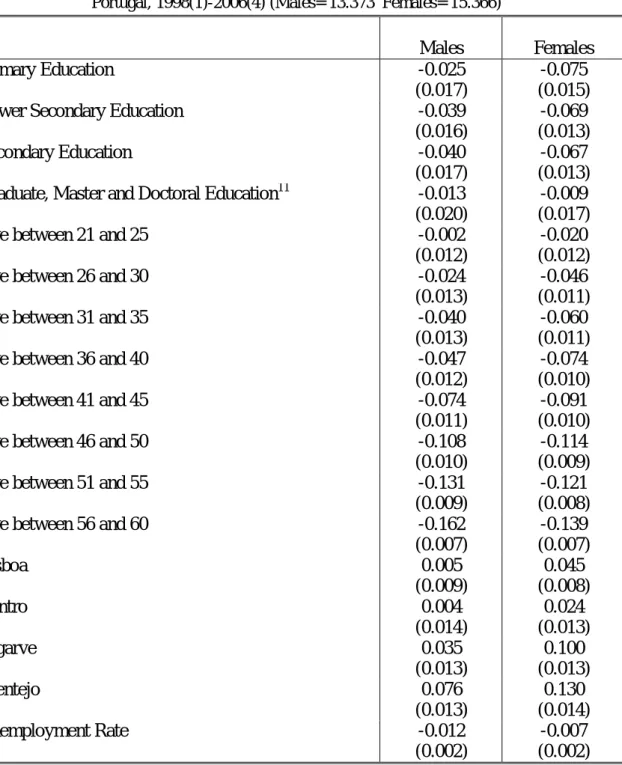
Table 1 exhibits the results for the marginal effects of the Job Finding Probability (JFP) using the IE dataset. The unemployment rate has a significant negative impact (-1.2% for males and -0.7% for females) in this probability implying a procyclical behaviour of JFP. Education and age also have a negative impact since more educated and older workers, males and females, have a lower JFP. Finally, all workers that work in a region other than Norte have a higher JFP.
13
Table 1: Marginal effects of the Probit estimation for the Job Finding Probability Portugal, 1998(1)-2006(4) (Males= 13.373 Females= 15.366)
Males Females
Primary Education -0.025
(0.017)
-0.075 (0.015)
Lower Secondary Education -0.039
(0.016) -0.069 (0.013) Secondary Education -0.040 (0.017) -0.067 (0.013) Graduate, Master and Doctoral Education11 -0.013
(0.020)
-0.009 (0.017)
Age between 21 and 25 -0.002
(0.012)
-0.020 (0.012)
Age between 26 and 30 -0.024
(0.013)
-0.046 (0.011)
Age between 31 and 35 -0.040
(0.013)
-0.060 (0.011)
Age between 36 and 40 -0.047
(0.012)
-0.074 (0.010)
Age between 41 and 45 -0.074
(0.011)
-0.091 (0.010)
Age between 46 and 50 -0.108
(0.010)
-0.114 (0.009)
Age between 51 and 55 -0.131
(0.009)
-0.121 (0.008)
Age between 56 and 60 -0.162
(0.007) -0.139 (0.007) Lisboa 0.005 (0.009) 0.045 (0.008) Centro 0.004 (0.014) 0.024 (0.013) Algarve 0.035 (0.013) 0.100 (0.013) Alentejo 0.076 (0.013) 0.130 (0.014) Unemployment Rate -0.012 (0.002) -0.007 (0.002) 11
14
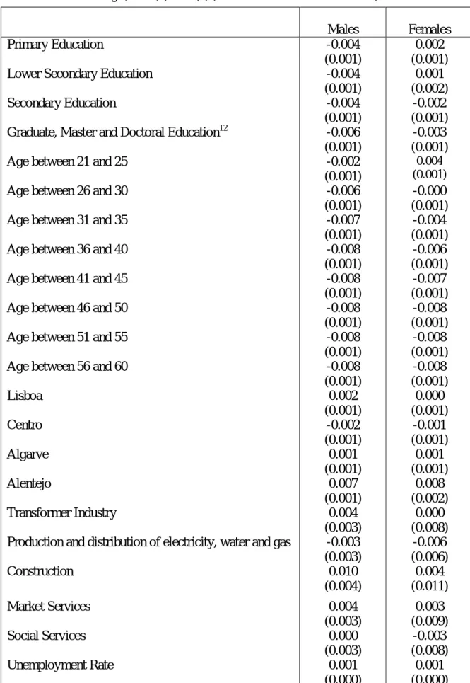
Table 2: Marginal effects of the Probit estimations for Job Separation Probability Portugal, 1998(1)-2006(4) (Males=167.933 Females=156.395)
12
All levels of education that are higher than or equal to a graduate level
Males Females
Primary Education -0.004
(0.001)
0.002 (0.001)
Lower Secondary Education -0.004
(0.001) 0.001 (0.002) Secondary Education -0.004 (0.001) -0.002 (0.001) Graduate, Master and Doctoral Education12 -0.006
(0.001)
-0.003 (0.001)
Age between 21 and 25 -0.002
(0.001)
0.004 (0.001)
Age between 26 and 30 -0.006
(0.001)
-0.000 (0.001)
Age between 31 and 35 -0.007
(0.001)
-0.004 (0.001)
Age between 36 and 40 -0.008
(0.001)
-0.006 (0.001)
Age between 41 and 45 -0.008
(0.001)
-0.007 (0.001)
Age between 46 and 50 -0.008
(0.001)
-0.008 (0.001)
Age between 51 and 55 -0.008
(0.001)
-0.008 (0.001)
Age between 56 and 60 -0.008
(0.001) -0.008 (0.001) Lisboa 0.002 (0.001) 0.000 (0.001) Centro -0.002 (0.001) -0.001 (0.001) Algarve 0.001 (0.001) 0.001 (0.001) Alentejo 0.007 (0.001) 0.008 (0.002) Transformer Industry 0.004 (0.003) 0.000 (0.008) Production and distribution of electricity, water and gas -0.003
(0.003) -0.006 (0.006) Construction 0.010 (0.004) 0.004 (0.011) Market Services Social Services Unemployment Rate 0.004 (0.003) 0.000 (0.003) 0.001 (0.000) 0.003 (0.009) -0.003 (0.008) 0.001 (0.000)
15
Table 2 presents the results for Job Separation Probability (JSP). Unemployment rates have a positive impact in the JSP (0.1% for both genders), reflecting a countercyclical behaviour of this probability. Higher education has a negative impact in JSP for males, while for females only the two highest levels have a lower JSP (Secondary Education and Graduate, Master and Doctoral Education). Age has the same negative impact in males and females. Except Centro, all regions have a higher JSP than Norte for both males and females.
As explained earlier, the coefficients for each variable are now estimated, which allow us to compute the probabilities for workers in the QP data set.
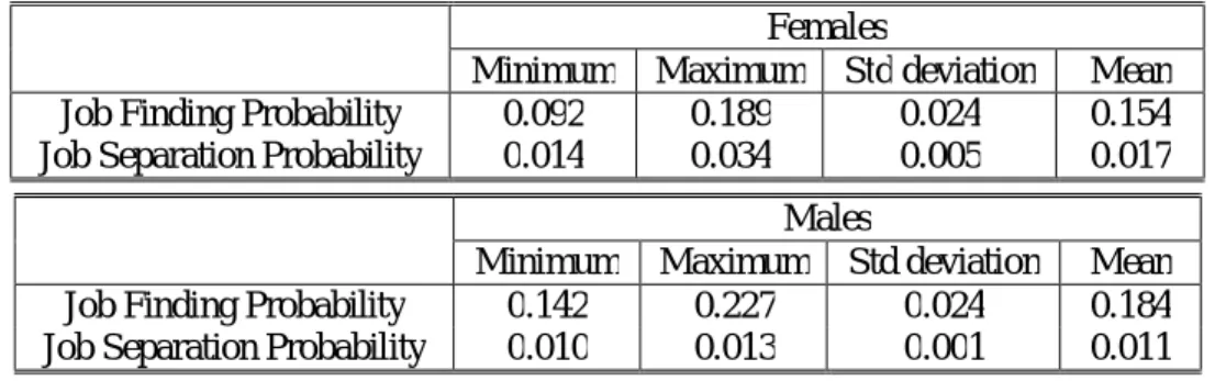
Table 3 shows the range of values for these probabilities. Job Finding Probability has a higher mean and volatility than Job Separation Probability. The mean values of JFP and JSP are respectively 18.4% and 1.1% for males, and 15.4% and 1.7% for females.
Table 3: Job finding and Job Separation Probabilities for workers in QP data set Portugal, 1986-2006 (N=13.740.886)
The fluctuations of Job Finding Probability and Job Separation Probability as the contribution of each flow to unemployment volatility are being subject to a significant number of studies.
Shimer (2005b) argues in favour of Job Finding Probability being highly procyclical and Job Separation Probability slightly countercyclical, aside from 1980 onwards, when it becomes simply acyclic. Therefore, unemployment volatilities are mainly generated
Females
Minimum Maximum Std deviation Mean Job Finding Probability 0.092 0.189 0.024 0.154 Job Separation Probability 0.014 0.034 0.005 0.017
Males
Minimum Maximum Std deviation Mean Job Finding Probability 0.142 0.227 0.024 0.184 Job Separation Probability 0.010 0.013 0.001 0.011
16
by the flows out, while the impact of the flows in is irrelevant. These findings support the beliefs that Mortensen and Pissarides’ (1994) model does not explain unemployment volatility.
Elsby, Michaels, Solon (2009) replicated Shimer´s calculations, finding out that the flow out of unemployment is highly procyclical with a significant impact in unemployment’s volatilities. Elsby el al. (2009) also noticed that the flow in is not acyclic as, it has a countercyclical behaviour in most recessions. These authors conclude that a “Complete understanding of cyclical unemployment requires an explanation of
countercyclical unemployment inflow rate as well as procyclical outflow rate”.
According to Elsby, Michaels and Solon (2009), Shimer (2005b) reached different conclusions due to the use of aggregate data, which does not take into account the worker heterogeneity. When unemployment flows are disaggregated, it is possible to see the existence of three different types of workers: job losers, job leavers and job entrants. These three types of workers have a procyclical flow out, specially the job losers, with a higher flow. No problem arises from the aggregation of the outflow rates because they go in the same direction. The same conclusion cannot be reached regarding the inflow rate, since job losers have a countercyclical inflow rate, job leavers a procyclical rate and finally job entrants flow in is acyclic. When the job separation probability is aggregated, the flows that go in opposite directions cancel each other, leading to a wrong conclusion that the flow in is acyclic.
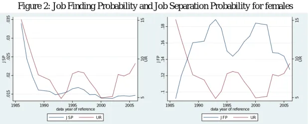
This study takes into account these types of workers heterogeneity by computing Job Finding and Job Separation probabilities at the individual level. Figure 1 and 2 shows the behaviour of unemployment rate with JSP and JFP. JSP and unemployment rate present a similar behaviour. When JSP increases the unemployment rate follows this increase. On the other hand when JFP increases the unemployment rate goes in the
17 3 4 5 6 7 U R .0 1 .0 1 1 .0 1 2 .0 1 3 J S P 1985 1990 1995 2000 2005
data year of reference
JSP UR 3 4 5 6 7 U R .1 4 .1 6 .1 8 .2 .2 2 J F P 1985 1990 1995 2000 2005
data year of reference
JFP UR 5 1 0 1 5 U R .0 1 5 .0 2 .0 2 5 .0 3 .0 3 5 J S P 1985 1990 1995 2000 2005
data year of reference
JSP UR 5 1 0 1 5 U R .1 .1 2 .1 4 .1 6 .1 8 J F P 1985 1990 1995 2000 2005
data year of reference
JFP UR
opposite direction. The results in table 4 support these conclusions showing the correlation between these probabilities and the unemployment rate.
Overall, table 4 and figure 1 and 2 show that both flows explain the unemployment rate and react to economic conditions, for both males and females. The flow that explains better unemployment, for males, is the flow out and for females is the flow in. These conclusions are achieved in part due to the fact that the unemployment rate is already in the computation of JFP and JSP.
Figure 1: Job Finding Probability and Job Separation Probability for males
18 Table 4:
Correlation between unemployment rate and job finding and job separations probabilities
Males Females
Job Finding Probability -0.4497 -0.2709
Job Separation Probability 0.2272 0.2799
4.2. Real Wage Cyclicality
The reaction of real wages to the business cycle is estimated using equation (3).
The nominal wage is calculated dividing the total regular payroll13 by the total number of hours. This ratio represents the hourly earnings. Real wage is then computed deflating the hourly earnings by the Consumer Price Index (CPI) at prices of 1986. The logarithm of this real wage is the dependent variable. This estimation takes into account work experience, using age and its square, as well as region and education of the worker.
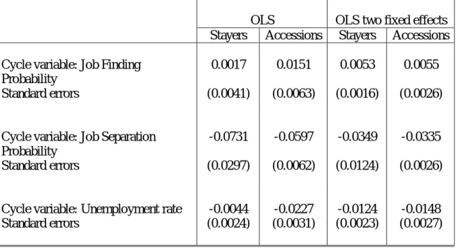
Table 5 contains the results for the wage cyclicality for males, using three different cyclical variables: Job Finding Probability, Job Separation Probability and Unemployment Rate.
Despite the difference in the magnitude of the response of real wages with the three indicators, the direction is the same: real wages are procyclical.
With an increase of 1 percentage point (p.p.) by Job Finding Probability, controlling for worker and firm heterogeneity, real wages increase by 0.53% for stayers and 0.55% for newly hired workers. The impact of this probability in real wages is somewhat limited, since in the analyzed period, JFP can increase by 8.5 p.p. 14 at most. Therefore the highest increase of real wages due to changes in this probability is 4.5% for stayers and 4.7% for newly hired.
13
Includes base wage, seniority payments and regular benefits
14
19
The impact of Job Separation Probability in real wages appears to be higher, since the elasticity between this probability and real wages is -3.49% for stayers and -3.35% for newly hired.
The highest possible in JSP in this period is 0.3 p.p. 15 which implies a maximum decrease of real wages by 1.05% for stayers and 1.01% for newly hired.
Finally, unemployment rate has a semi elasticity of -1.24% for stayers and -1.48% for newly hired, controlling for firm and worker heterogeneity.
When real wage cyclicality is estimated only using OLS, without controlling for worker and firm heterogeneity, these results change, showing the importance of the two fixed effects.
Table 5: Real wage reaction to the JSP, JFP and unemployment rate for males Portugal, 1986-2006 (N=13.740.886)
Dependent variable: log of real hourly earnings
OLS OLS two fixed effects Stayers Accessions Stayers Accessions Cycle variable: Job Finding
Probability
0.0017 0.0151 0.0053 0.0055 Standard errors (0.0041) (0.0063) (0.0016) (0.0026)
Cycle variable: Job Separation Probability
-0.0731 -0.0597 -0.0349 -0.0335 Standard errors (0.0297) (0.0062) (0.0124) (0.0026)
Cycle variable: Unemployment rate -0.0044 -0.0227 -0.0124 -0.0148 Standard errors (0.0024) (0.0031) (0.0023) (0.0027)
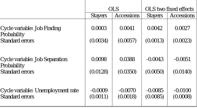
Table 6 shows the results of the real wage cyclicality for females with the same three cyclical indicators as used for males. The real wage of female workers is procyclical as
15
20
the males real wage. The results on the real wage cyclicality of newly hired workers are the only ones that are not similar for males and females. A newly hired male worker has a more cyclical real wage than a worker in an ongoing job with JFP and unemployment rate. For females, the cyclical variables that create a higher real wage cyclicality for the same type of workers, are the JSP and the unemployment rate.
Table 6: Real wage reaction to the JSP, JFP and unemployment rate for females Portugal, 1986-2006 (N= 9.112.126)
Dependent variable: log of real hourly earnings
OLS OLS two fixed effects Stayers Accessions Stayers Accessions Cycle variable: Job Finding
Probability
0.0003 0.0041 0.0042 0.0027 Standard errors (0.0034) (0.0057) (0.0013) (0.0023)
Cycle variable: Job Separation Probability
0.0098 0.0388 -0.0043 -0.0051 Standard errors (0.0128) (0.0350) (0.0050) (0.0140)
Cycle variable: Unemployment rate -0.0009 -0.0070 -0.0085 -0.0100 Standard errors (0.0011) (0.0018) (0.0085) (0.0008)
The only paper that tried to study the reaction of real wages to the flow in and out was Carneiro, Guimarães and Portugal (2009), but their conclusions are slightly different from the ones found in this study. These authors also concluded that real wages have a procyclical behaviour with the three cyclical components, but the reaction of real wages in their study is higher than the one find in this study. This difference can be explained by the fact that the Job Finding and Job Separation Probabilities in the former study were computed at the aggregated level while in this study we calculate them at the individual one.
21
5. Conclusion
The purpose of this study is the creation of a disaggregated cyclical variable to be used in the estimation of real wage cyclicality. This new cyclical component, allied with the use of two unique data sets provide a very robust evidence on real wage cyclicality which is such a challenging topic.
In the best of our knowledge, real wage cyclicality was never tested using the kind of disaggregated variables created in this study. The use of this type of cyclical variables has a major importance mainly for one reason. This reason is the information gain obtained from the creation of a personal cyclical measure for each individual, since economic conditions have a higher or lower impact in each worker depending on his/her characteristics.
We build two cyclical components based on the decomposition from the search and matching model, the Job Separation Probability and Job Finding Probability. Therefore this study has four main conclusions:
First, Job Finding Probability and Job Separation Probability have the expected behaviour to the business cycle. While Job Finding Probability has a procyclical reaction to the business cycle, Job Separation Probability reacts negatively to the business cycle, having then a countercyclical behaviour. We also find evidence that volatilities of unemployment are explained by both probabilities which is, in part, against Shimer (2005b) arguments that the flow out is the only flow that explains these volatilities.
Second, real wages are procyclical for both genders and for all workers irrespective of the three cyclical components: Job Finding Probability, Job Separation Probability and the unemployment rate. The real wage of stayers male workers, controlling for worker and firm heterogeneity, changes by 0.53%, -3.49% and -1.24% when the Job Finding
22
Probability, Job Separation Probability and unemployment rate increase by 1 p.p. respectively. For the same type of female workers, an increase of 1 p.p. in Job Finding Probability, Job Separation Probability and unemployment rate changes their real wage by 0.42%, -0.43% and -0.85% respectively.
Third, the results on the magnitude of real wage cyclicality for newly hired workers are ambiguous. The real wage of this type of male worker has an elasticity with respect to the Job Finding Rate and Job Separation Rate of 0.55% and -3.35%, respectively, and a semi elasticity with respect to the unemployment rate of -1.48%. Recently hired male workers have a more responsive real wage than a male worker in a continuing job when the Job Finding Probability and the unemployment rate are the cyclical variables used in the estimation of real wage cyclicality. Newly hired female workers also have a more cyclical real wage with the unemployment rate but, contrary to males, Job Separation Probability creates a higher real wage cyclicality for this type of female workers.
Finally, the conclusions in this study support the findings of Pissarides (2007) and Haefke et al. (2007) that the business cycle fluctuations in unemployment and vacancies cannot be explain by real wage rigidity. Despite the ambiguous conclusions about the degree of the real wage cyclicality for newly hired workers, these workers have a real wage that reacts strongly to the business cycle. Therefore, the real wage rigidity does not appear to be a convincing solution to the unemployment volatility puzzle.
23
References
1. Abraham, K. and J. Haltiwanger (1995), “Real Wages and the Business Cycle”, Journal of Economic Literature, Vol. 33, pp. 1215-1264.
2. Barlevy, G. (2001), “Why Are the Wages of Job Changers So Procyclical?”, Journal of Labor Economics, Vol. 19, pp. 837-878.
3. Barro, R. and R. King (1984), "Time- Separable Preferences and Intertemporal-Sub-stitution Models of Business Cycles," The Quarterly Journal of Economics, Vol. 99, No. 4, pp. 817-839
4. Beaudry, P. and J. DiNardo (1991), “The Effect of Implicit Contracts on the Movement of Wages over the Business Cycle: Evidence from Micro Data”, Journal of Political Economy, Vol. 99, pp. 665-688.
5. Bils, M. (1985), “Real Wages over the Business Cycle: Evidence from Panel Data”, Journal of Political Economy, Vol. 93, pp. 666-689.
6. Brandolini, A. (1995), “In Search of a Stylised Fact: Do Real Wages Exhibit a Consistent Pattern of Cyclical Variability?”, Journal of Economic Surveys, Vol. 9, pp. 103-163.
7. Carneiro, A., Guimarães P. and P. Portugal (2009), "Real Wages and the Business Cycle: Accounting for Worker and Firm Heterogeneity," IZA Discussion Papers 4174, Institute for the Study of Labor (IZA).
8. Cardoso, A. and P. Portugal (2005), "ContractualWages and theWage Cushion under Different Bargaining Settings", Journal of Labor Economics, Vol. 23, pp. 503-523.
9. Elsby, M., Ryan, M., G. Solon (2009), “The Ins and Outs of Cyclical Unemployment.”, American Economic Journal: Macroeconomics, Vol. 1, No.1, pp. 84–110.
24
10. Guimarães, P., P. Portugal, 2009. "A Simple Feasible Alternative Procedure to Estimate Models with High-Dimensional Fixed Effects," IZA Discussion Papers 3935, Institute for the Study of Labor (IZA).
11. Hall, R. (2005), "Employment Fluctuations with Equilibrium Wage Stickiness", American Economic Review, Vol. 95, pp. 50-65.
12. Haefke, C., Sonntag, M., T. Rens (2007), “Wage rigidity and job creation” IZA discussion papers number 371
13. Keane, M., R. Moffitt and D. Runkle (1988), “Real Wages over the Business Cycle: Estimating the Impact of Heterogeneity with Micro Data”, Journal of Political Economy, Vol. 96, pp. 1236-1266.
14. Keynes, J. (1939), “Relative Movements of Real Wages and Output”, Economic Journal, Vol. 49, pp. 34-51.
15. Lucas, Robert E., JR. (1977), "Understanding Business Cycles," J. Monet. Econ., Supplementary Series 1977, 5, pp. 7-29.
16. Mitchell, M., M. Wallace and J. Warner (1985), “Real Wages over the Business Cycle: Some Further Evidence”, Southern Economic Journal, Vol. 51, pp. 1162-1173.
17. Mortensen, D. and C. Pissarides (1994), "Job Creation and Job Destruction in the Theory of Unemployment", Review of Economic Studies, Vol. 61, pp. 397-415.
18. Okun (1973), “Upward Mobility in a High-pressure Economy”, Brookings Papers on Economic Activity, Vol. 1, pp. 207-252.
19. Pissarides, C. (2000), “Equilibrium Unemployment Theory”, 2nd. Ed., Cambridge, MA, MIT Press.
25
20. Pissarides, C. (2007), “The Unemployment Volatility Puzzle: Is Wage Stickiness the Answer?” CEP Discussion Papers number dp0839
21. Shimer, R. (2004), "The Consequences of Rigid Wages in Search Models", Journal of the European Economic Association, Vol. 2, pp.469-479.
22. Shimer, R. (2005a), "The Cyclical Behavior of Equilibrium Unemployment and Vacancies", American Economic Review, Vol. 95, pp. 25-49.
23. Shimer, R. (2005b). “Reassessing the Ins and Outs of Unemployment” NBER Working Papers number 13421
24. Smyth, G. (1996), “Partitioned Algorithms for Maximum Likelihood and other non-linear Estimation”, Statistics and Computing, Vol.6, pp. 201-216 25. Solon, G., R. Barsky and J. Parker (1994), “Measuring the Cyclicality of
Real Wages: How Important is Composition Bias?”, Quarterly Journal of Economics, Vol. 109, pp. 1-25.
APPENDIX A
This appendix provides a simple explanation about the estimation technique used in this study.
Controlling for group and individual heterogeneity while using extremely large data sets, such as the one used in this study, may pose a challenging computational problem. The number of dummy variables required to appropriately capture heterogeneity makes the usual estimation methods computationally too demanding.
However there is an estimation technique that solves the computational problem and yields a solution equivalent to OLS: the partitioned algorithm16. A simple example showing how this algorithm works is presented below.
16
26
A study wants to estimate equation A1 with only one fixed effect
= + + (A1)
Where X is an M x k matrix, D is a M x n dummy matrix and and are the vector of the unknown parameters. OLS estimators can be computed by minimizing the square of the residuals. In order to do so a set of equations known as the normal equations is required. A generic form of these equations is given below:
= (A2)
Solving each equation
= ( ) ( − )
= ( ) ( − ) (A3)
Estimation of a given vector of coefficients, or , is much easier if the least square solution of the other is known. Therefore the partitioned algorithm solution is based on the following iteration:
1. Find the initial values for regressing of on
2. Compute the normal equation for with the previous estimation of and then estimate
3. Estimate again the normal equation for taking into account the value of found in 2.
27
The outcome of this algorithm will be exactly equal to the OLS solution but in a feasible way. The method can be easily adjusted to take into account two fixed effects it would simply imply more interactions.17
The standard errors for the unemployment rate are corrected to the lack of cross-sectional variation using an annual clustered standard errors.
17