The influence of geometric factors on the wall shear stress distribution in realistic human coronary arteries

(1)

DEPARTAMENTO DE FÍSICA

The influence of geometric

factors on the wall shear

stress distribution in

realistic human coronary

arteries

Jorge André Piedade Pinhal dos Santos

Dissertação apresentada na Faculdade de Ciências e Tecnologia da Universidade Nova de Lisboa para a obtenção do grau de Mestre em Engenharia Biomédica.

A presente dissertação foi desenvolvida no Erasmus Medical Center em Roterdão, Holanda.

Orientadora:

Dr. Ir. Jolanda J. Wentzel

Lisboa

(2)

Acknowledgments

In the first place I would like to thanks Dr. Ir. Jolanda Wentzel for her

supportive supervision and for her patience for reading and correcting all the drafts I

have written during this period.

My special thanks to Diana and Sandro, my cousins, and to “our Portuguese group” in Rotterdam, who helped and supported me during these six months abroad.

I would also like to thank all the researchers and colleagues in the

Biomechanics Laboratory in the Erasmus MC, who welcomed me and treated me as

one of them.

Thanks also to all of my friends, especially to Samuel, Eduardo, Daniel, Barros,

Filipa, Sara, Osório and Hugo, without whom, the last five years wouldn’t have been so much fun and unforgettable.

To Inês, my special thanks for all the care and courage given. You are my ally.

Finally, my most special thanks to my brother Pedro, and my parents Luís and

(3)

Jorge Santos iii

Abstract

Background:

Atherosclerosis is the main cause of death in the Western society. It is a geometrically focal disease, affecting preferentially vessel areas of low wall shear stress (SS), which induces the expression of atherogenic genes. To predict wall SS several options are available. Among them Computational Fluid Dynamics (CFD) simulations on 3D reconstructed coronaries using Finite Element Modeling (FEM). However, to perform CFD a 3D representation is needed. To obtain a 3D representation of the coronary under study different methods can be applied.

Methods:

CFD calculations were performed using FEM on ten 3D reconstructed coronary arteries by the state-of-the-art ANGUS method (biplane angiography + Intravascular Ultrasound (IVUS)). The SS outcomes of the CFD calculations were compared with SS calculated by the Poiseuille equation, and with the SS outcomes of CFD simulations of the same 3D reconstructed arteries by QCA-3D (biplane angiography – no cross-sectional information) and Straight (IVUS images stacked on a straight centerline – no curvature information) methods.

Results:

The Poiseuille equation did not have any sensitivity in predicting any low SS (<0.5 Pa) per cross-section. However, the average correlation coefficient between the average SS per cross section from the Angus geometries and SS based on the Poiseuille equation was r2 = 0.65  0.09. A strong correlation was obtained for the SS from the ANGUS and the Straight method, while only an average correlation was obtained between ANGUS and QCA-3D average SS. Bland-Altman analysis was performed to confirm the results agreement. The sensitivity and specificity of the QCA-3D and Straight method in predicting low and high SS was measured. Geometric factors, such as local curvature, area gradient and torsion were found to be related to the presence of SS peaks or to regions prone to plaque development. These geometric risk factors were utilized to give some guidelines on meshing optimization.

Conclusions:

(4)

Resumo

Introdução:

A aterosclerose é a principal causa de morte na sociedade ocidental. É uma doença geometricamente focal que afecta preferencialmente áreas da parede de vasos com baixa tensão de cisalhamento, induzindo a expressão de genes aterogénicos. Hoje em dia para prever a tensão de cisalhamento (SS) da parede arterial várias opções são viáveis. Entre elas, simulações de Dinâmica de Fluidos Computacional (CFD) em coronárias reconstruídas em 3D em conjugação com Modelação em Elementos Finitos (FEM). Assim sendo, para realizar cálculos CFD, a representação 3D das coronárias é necessária. Para obter estas representações 3D vários métodos podem ser usados.

Métodos:

Os cálculos CFD são realizados usando FEM em dez artérias coronárias reconstruídas em 3D pelo método padrão ANGUS (angiografia biplanar + Ultrassom Intravascular (IVUS)). Os valores de SS obtidos nos cálculos CFD são comparados com os valores de SS calculados pela equação de Poiseuille, e com o SS obtido pelos cálculos CFD para as mesmas artérias coronárias, mas reconstruídas em 3D pelo método QCA-3D (angiografia biplanar – sem informação sobre a forma de cada secção de corte) e pelo método Straight (imagens IVUS empilhadas ao longo de um eixo recto – sem informação da curvatura).

Resultados:

A equação de Poiseuille não tem sensibilidade para prever um valor de SS baixo (SS<0.5) em cada secção de corte. Contudo, o coeficiente de correlação média, entre o valor médio de SS em cada secção de corte por geometrias Angus e SS baseado na equação de Poiseuille são r2₌

0.65  0.09. Uma forte correlação foi obtida a partir dos valores de SS obtido com ANGUS e o pelo método Straight, enquanto apenas foi obtida uma correlação média entre o SS médio por corte entre o método ANGUS e o método QCA-3D. Uma análise Bland-Altman foi realizada para confirmar a concordância dos resultados. A sensibilidade e a especificidade do método QCA-3D e do método Straight para prever baixos e altos valores de SS foram medidas. Factores geométricos, como a curvatura local, o gradiente em área e a torção foram relacionados com a presença de picos de SS ou com regiões propensas ao desenvolvimento de placas. Estes factores de risco geométricos foram usados para dar algumas orientações para optimização das malhas de elementos finitos.

Conclusões:

(5)

Jorge Santos v

Abbreviations list

ANGUS– Angiography + Intravascular ultrasound

CAAS– Cardiovascular Angiography Analysis System

QCA-3D–Quantitative Coronary Analysis 3D

CFD – Computational Fluid Dynamics

De– Dean Number

eNOS– Endothelial nitric oxide synthase

ESS– Endothelial Shear Stress

FDA– Food and Drug Administration

FEM– Finite Element Method

IVUS– Intravascular ultrasound

LAD– Left anterior descending artery

LCA– Left coronary artery

LCX– Left circumflex artery

LDL– Low density lipoprotein

LMCA– Left main coronary artery

RCA– Right coronary artery

Re– Reynolds number

SS– Shear stress

(6)

List of figures

Figure 1.1 - Main coronary arteries... 14

Figure 1.2 - Arterial wall layers ... 15

Figure 1.3 - Healthy human artery vs. artery narrowed by atherosclerotic plaque ... 16

Figure 1.4 - Clot formation on a coronary artery ... 17

Figure 1.5 - Definition of endothelial shear stress [7] ... 17

Figure 1.6 - Atheroprotective vs. atherogenic phenotype [5] ... 19

Figure 1.7 - Eccentric plaque regions [10] ... 19

Figure 1.8 - Poiseuille flow (velocity) profile ... 22

Figure 1.9 - Different flow profiles (adapted from Christian Poelma’s Biological Fluid Mechanics lecture on Blood tissue interaction; the role of wall shear stress. Delft University of Technology)[16] ... 22

Figure 1.10 - A) IVUS images of a RCA; B) Angiographic image from the same artery; C) 3D reconstruction [18] ... 24

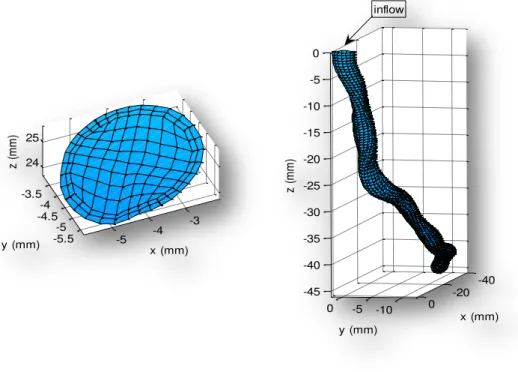
Figure 2.1 - ANGUS, QCA-3D, Straight and Poiseuille – 3D Reconstructions example and a corresponding cross-section from each method. ... 26

Figure 3.1 - Example of the finite element mesh of a coronary artery ... 28

Figure 4.1 - 3D reconstruction of a left anterior descending artery by the ANGUS method (in the left) and a Poiseuille cylinder with the same cross sectional area .... 33

Figure 4.2 - Average SS vs. Lumen Area plots ... 34

Figure 4.3 - Average SS vs. Lumen Area, based on the CFD calculations (o) and the Poiseuille formula (-) ... 35

Figure 4.4 - Poiseuille shear stress versus Average shear stress – Influence of blood flow ... 36

Figure 4.5 - Poiseuille and Average SS scatter plots for 100%, 50%, 10% and 1% of physiological blood flow ... 37

Figure 4.6 - Average r2– Average SS vs. Poiseuille SS ... 38

Figure 4.7 - Bland-Altman plot (ANGUS vs Poiseuille) ... 39

Figure 4.8 - Local Wall SS Histogram ... 40

(9)

Jorge Santos ix Figure 4.10 - Velocity profiles for different blood flows (100%, 50%, 10% and 1%) for

a stenotic cross section ... 43

Figure 4.11 - Velocity profiles for different blood flows (100%, 50%, 10% and 1%) for

a “normal” cross section... 43

Figure 5.1 - 3D reconstructions of a left anterior descending artery by the ANGUS (in

the left) and the QCA-3D techniques ... 44

Figure 5.2 - Average SS vs Lumen Area plots from ANGUS (o) and QCA-3D (o) ... 45

Figure 5.3 - Lumen area and average SS per cross section from ANGUS and QCA-3D46

Figure 5.4 - Correlation between Average SS from ANGUS and QCA-3D ... 46

Figure 5.5 - Bland-Altman plot of the average SS per cross section ... 47

Figure 5.6 - Lumen Area, Maximum, Average and Minimum SS per cross section –

ANGUS vs QCA-3D (example) ... 48

Figure 5.7 - Bland-Altman plot – Maximum SS per cross section ... 49 Figure 5.8 - Local wall SS histogram (ANGUS vs QCA-3D) ... 50

Figure 5.9 - Example of a vessel with low SS elements (<0.5 Pa) for the ANGUS, the

QCA-3D method and the overlapping cross-sections. ... 51

Figure 5.10 - Example of a vessel with high SS elements (in this case <5.01 Pa) for the

ANGUS, the QCA-3D method and the overlapping cross-sections. ... 53

Figure 6.1 - 3D reconstruction of the curved ANGUS vessel (left) and from the

corresponding straight vessel (right) ... 54

Figure 6.2 - 3D view of the local wall SS distribution in both ANGUS original vessel

and in the straight vessel ... 55

Figure 6.3 - Lumen Area and Average SS comparison between ANGUS and Straight

vessels ... 56

Figure 6.4 - Lumen Area and Average SS comparison between ANGUS and Straight

vessels ... 56

Figure 6.5 - Bland-Altman plot of the average SS per cross section for all patients .. 58

Figure 6.6 - Lumen Area, Average SS and Maximum SS per cross section comparisons,

between ANGUS and Straight vessels ... 59

Figure 6.7 - Wall SS distribution of an ANGUS and a Straight geometry ... 60

Figure 6.8 - 3D view of the SS distribution in the reconstructed ANGUS and Straight

(10)

Figure 6.9 - Wall shear stress histogram (Angus vs Straight) ... 61

Figure 6.10 - Example of a vessel with elements with low SS (<0.5 Pa) for the ANGUS, the Straight method and the overlap of both ... 63

Figure 6.11 - Example of a vessel with low SS elements (<0.5 Pa) for the ANGUS, the Straight method and the overlapping cross-sections ... 64

Figure 6.12 - Example of a vessel with elements with high SS (>9.32 Pa) for the ANGUS and the Straight method, and the overlap of both ... 66

Figure 6.13 - Example of a vessel with elements with high SS (>9.32 Pa) for the ANGUS and the Straight method, and the overlapping cross-sections. ... 67

Figure 6.14 - Wall SS distribution an ANGUS and a Straight geometry ... 68

Figure 6.15 - Mean Longitudinal SS for ANGUS and the Straight vessel (p060362) ... 68

Figure 6.16 - Longitudinal Shear Stress ... 69

Figure 7.1 - Average SS Gradient vs Lumen Area Gradient ... 72

Figure 7.2 - Example of the relation between the lumen area gradient and the gradient in SS ... 73

Figure 7.3 - Lumen area gradient and average SS per cross section along a coronary length ... 74

Figure 7.4 - Example of the relation between the lumen area gradient and the local SS ... 74

Figure 7.5 - Curvature parameters ... 75

Figure 7.6 - Curvature radius vs. maximum SS per cross-section ... 76

Figure 7.7 – Dean Number vs. maximum SS per cross-section ... 76

Figure 7.8 - Highlight of the dots deviated from the line based on the Poiseuille equation ... 77

(11)

Jorge Santos xi

List of tables

Table 1.1 - Mean diameters of the main coronaries according to Mosseri et al. [2] . 14

Table 3.1 - Patients, corresponding coronaries and some geometric and flow features

of the ANGUS reconstructed vessels... 27

Table 3.2 - Inflow rate and pressure (in and out) values for the CFD calculations ... 29

Table 3.3 – Measure of sensitivity and Specificity ... 32

Table 4.1 - Correlation coefficients (r2) ... 38

Table 4.2 - Bland-Altman statistic results ... 39

Table 4.3 - Average SS from CFD calculations and Poiseuille SS for the 57th cross section of patient p060233. Re is an abbreviation for Reynolds number ... 42

Table 5.1 - Average Shear Stress correlation parameters ... 47

Table 5.2 - Correlation coefficients (r2) for the Maximum SS per cross section ... 49

Table 5.3 – Cross-sections with low SS (<0.5 Pa) by ANGUS and QCA-3D method .... 50

Table 5.4 – High SS threshold for all patients. ... 52

Table 5.5 - Percentage of cross sections with high SS (>x Pa) in the ANGUS and QCA-3D method ... 53

Table 6.1 - Correlation coefficients (r2) for the Average and Maximum SS per cross section ... 57

Table 6.2 - Bland-Altman analysis results for all patients individually ... 58

Table 6.3 - Percentage of elements with low SS (<0.5 Pa) in the ANGUS and Straight method ... 62

Table 6.4 - Percentage of cross sections with low SS (<0.5 Pa) in the ANGUS and Straight method ... 63

Table 6.5 - Elements with high SS (>x Pa) in the ANGUS and Straight method .. 65

Table 6.6 - Percentage of cross sections with high SS (>x Pa) in the ANGUS and Straight method ... 67

Table 6.7 - Average longitudinal SS ... 69

Table 7.1 - Average SS Gradient vs Lumen Area Gradient – correlation coefficient and linear regression line slope and y-intercept ... 72

(12)

Table 11.2 - Some geometric and flow parameters of the QCA-3D reconstructed

vessels ... 91

Table 11.3 - Some geometric and flow parameters of the Straight reconstructed

(13)

Jorge Santos 13

Introduction

The research to this Master Dissertation in Biomedical Engineering was

performed at the Biomechanics Laboratory of the Biomedical Engineering

Department, which is part of the Thoraxcenter of the Erasmus Medical Center in

Rotterdam, The Netherlands. The supervisor of this project and head of the

Biomechanics Lab. is Dr. ir. Jolanda J. Wentzel. The Biomedical Engineering is a

research group focused on the cardiovascular diseases, namely on its origin,

diagnosis and treatment. The Biomedical Engineering is, then, divided in the

Experimental Echocardiography group and the Biomechanics Lab. At the latest,

researchers study the effects of the mechanical stresses on the development and

progression of vascular disease, namely atherosclerosis. The research includes cell

studies, animal experiments and patient studies. In order to study the relationship

between biomechanical parameters and vascular disease is used the combination of

imaging modalities and computer modeling, resulting in applications such as ANGUS.

Chapter 1. Background

1.1. Coronary Arteries

The coronary arteries are the vessels that supply blood rich in oxygen to the

heart muscle. Only the main coronary arteries lie on the surface of the heart as the

smaller arteries penetrate the surface into the cardiac muscle. The two main

coronaries are the left coronary artery (LCA) and the right coronary artery (RCA),

which derive directly from the aorta. The LCA then bifurcates into the left circumflex

artery (LCX) and the left anterior descending artery (LAD) (see figure 1.1). The length

of the LCA ranges from 1 to 25 mm, when it bifurcates into the LAD whose length

varies from 10 to 13 cm and the LCX, which measures 6 to 8 cm in length. The RCA

measures about 12 to 14 cm in length [1]. These vessels mean diameters and

(14)

Figure 1.1 - Main coronary arteries (http://cognitorex.blogspot.com/2007/06/i-got-new-stent-today.html)

Coronary Artery Mean Diameter (mm)  SD Range (mm)

LMCA 4.7  1.0 3.6 – 7.2

Proximal LAD 3.9  0.8 2.4 – 5.6 Distal LAD 1.7  0.4 1.2 – 2.7 LCX 3.4  0.8 1.5 – 5.2 Proximal RCA 3.6  0.8 2.0 – 4.8 Distal RCA 2.7  0.9 1.1 – 4.5

Table 1.1 - Mean diameters of the main coronaries according to Mosseri et al. [2]

The LCA supplies mainly the anterior and lateral portions of the left ventricle

while the RCA supplies most of the right ventricle and the posterior part of the left

ventricle in 80 to 90 percent of people [3].

The blood flow in coronary arteries is laminar, which means that it flows at a

steady rate through the vessels, with each layer of blood remaining at the same

distance from the wall. The central portion of the blood stays in the center of the

vessel [3]. Since the flow in coronary arteries is laminar, the Reynolds number is also

low. The non-dimensional Reynolds number is the measure of tendency for

turbulence to occur and it is represented by the following equation:

 vd 

Re (1)

(15)

Jorge Santos 15 does not occur at a specific Reynolds number, even though, if the Reynolds number

is below 2000 the fluid flow is laminar. Between 2000 and 4000 the flow is in

transition between laminar and turbulent flow, and if the Reynolds number is over

4000 the flow is considered to be completely turbulent. The typical Reynolds number

in coronary arteries is around 250[3].

1.2. Arterial Wall Anatomy

The arterial wall is composed of three layers (tunicas). As seen in figure 1.2,

the innermost layer is called tunica intima and consists of a single layer of

endothelial cells, connective tissue and some elastic fibers. The middle layer is called

tunica media and it consists mainly of smooth muscle cells and elastic fibers. The

outer layer is called tunica adventitia and is composed of collagen fibers as well as

other elastic fibers. The tunica adventitia is

the strongest of these three layers.

Anatomically, the arterial walls are stronger

than the venal walls, so they are less

distensible [4]. Also, atherosclerotic arteries

become hardened so they lose compliance.

1.3. Atherosclerosis

Atherosclerosis is the main cause of death in the developed world [5]. An

atherosclerotic plaque is formed by deposits of lipids, macrophages, cellular debris,

calcium, among other substances (see figure 1.3), in between the innermost layer

(called intima) and the intermediate layer (called media) of the arterial wall.

Atherosclerosis is generally associated with some risk factors, such as hypertension,

smoking, hyperlipidemia, sedentary lifestyle, viral infection, diabetes mellitus,

chronic infections and also with genetic predisposition [5].

Figure 1.2 - Arterial wall layers (http://www.nlm.nih.gov/medlineplus/en

(16)

The origin of an atherosclerotic

plaque is due to the excessive

accumulation of LDL (low-density

lipoprotein, also known as bad

cholesterol, and composed of

lipids and a protein) particles in

the arterial wall. Those LDL

particles undergo some chemical

alterations such as oxidation. The

cells in the vessel interpret these modified LDLs as a danger sign, so the endothelial

cells of the artery start to display adhesion molecules on their blood-facing surface.

These adhesion molecules attract monocytes and T cells in the blood into the intima,

where the monocytes mature into macrophages that will ingest the modified LDLs

and produce inflammatory mediators. The macrophages become filled with fatty

substances (they transform into foam cells) and along with the T cells they constitute

the early form of a plaque. A fibrous cap is formed over the lipid core and smooth

muscle cells migrate from the media to the top of the intima, multiply and produce a

fibrous matrix that glues the cells together [6]. These plaques can grow into the

artery lumen, restricting it, causing lumen narrowing, which can hamper the blood

delivery to the tissues. Vessel stenosis can provoke, among others, angina pectoris.

Plaques that are at high risk to rupture (called vulnerable plaques) are characterized

by a certain composition: necrotic core, inflammatory cells infiltration (macrophage

and T cells), large lipid pool and a thin fibrous cap. If a vulnerable plaque ruptures it

can cause a thrombus or a clot. If a clot is big enough it can block a blood vessel

causing a heart attack or a stroke, if it is a coronary or a brain artery respectively

(figure 1.4).

(17)

Jorge Santos 17

Figure 1.4 - Clot formation on a coronary artery

(http://64.143.176.100/library/healthguide/en-us/support/topic.asp?hwid=zm2431)

1.4. The role of shear stress in Atherosclerosis

Forces are inflicted on vascular tissues in different directions. There are

circumferential and radial forces (tensile or compressive), and there are tangential

forces such as shear. The endothelial shear stress (ESS) is the tangential force

derived by the friction of the flowing blood on the endothelial surface. It is the

product of the shear rate (difference of velocity between two different layers divided

by the distance between them, or dV/dr) at the wall and the blood viscosity (µ) [7].

dr dV

s 

 

Figure 1.5 - Definition of endothelial shear stress [7]

Due to the pulsatile nature of the blood flow and the geometric configuration

(18)

parts of the arteries the shear stress varies from 1.5 to 7 Pa [7]. Though, in irregular

regions, like outer walls of vessel bifurcations, the shear stress is usually low and

oscillatory, with values ranging from <1 to 1.2 Pa.

The endothelial cells of the arteries respond to the different range of shear

stress values in different ways. Even though the shear stress has magnitudes of only

5 Pa, the endothelial cells are specially equipped with a dedicated sensing

mechanism, the mechanoreceptors, which are capable to detect those shear stress

stimuli on the endothelial cells surface [8]. After detecting the shear stress stimulus,

a complex pathway known as mechanotransduction is activated.

Different patterns of shear stress induce different phenotypes of the

endothelial cells of the arteries. With physiological shear stress (>1.5 Pa), the

endothelial cells will show an atheroprotective phenotype, although, if the shear

stress is low and/or oscillatory (<0.4 Pa) the endothelial cells exhibit an atherogenic

phenotype [5] (see figure 1.6). The low shear stress causes a change in the

morphology of endothelial cells (which become less elongated and are not aligned

with the direction of the blood flow); the atherogenic phenotype is mainly

characterized by reduced production of eNOS (endothelial nitric oxide synthase, a

vasodilator), reduced endothelial repair, increased amounts of reactive oxygen

species, higher leukocyte adhesion (high expression of vascular cell adhesion

molecule-1 also known as VCAM-1), higher permeability to lipoproteins and higher

inflammation predisposition [9]. This atherogenic phenotype of the endothelial cells

combined with the presence of the systemic risk factors will promote the

atherosclerotic plaque formation at these sites.

Therefore, despite being associated with the risk factors mentioned above,

the atherosclerosis is also a geometrically focal disease [5], which affects

preferentially the areas where the shear stress caused by blood flow is low and

oscillating, like the outer edges of artery bifurcations, inner curvatures and close to

side branches. On the other hand, areas exposed to steady blood flow and higher

(19)

Jorge Santos 19

Figure 1.6 - Atheroprotective vs. atherogenic phenotype [5]

In addition to the role shear stress has in the atherosclerotic plaque

formation, it is thought that it also plays an important role in the development of

those plaques, into a quiescent or high-risk (vulnerable) atherosclerotic plaque [7,

10, 11].

As seen in figure 1.7 an eccentric vulnerable plaque can be divided in four

regions: upstream and downstream, the midcap and the lateral shoulders. The

upstream region of the plaque is submitted to high shear stress; meanwhile at the

downstream regions the shear stress is low.

(20)

When a plaque begins to grow, the lumen narrowing is prevented by outward

vessel remodeling [10], in order to maintain normal values of shear stress. However,

this vessel remodeling has some consequences. It can promote the plaque growth or

even the plaque rupture. The plaque growth can occur in the downstream region of

the plaque, due to low shear stress, which favors the atherosclerotic progression.

The plaque fissuring occurs mainly at the upstream lateral plaque shoulders, and it is

suggested that the high shear stress can be a reason for it, as it stimulates the

endothelium to thin the fibrous cap [10]. Subsequently the tensile stress causes the

plaque disruption at the lateral shoulders, because at those regions the fibrous cap is

thinner and has, consequently, less resistance to tensile strength [12]. As the tensile

stress is cyclic (due to oscillations in blood pressure), it can also lead to cap fatigue

and rupture [12].

Thus it is important to continue studying new approaches on estimating wall

shear stress in coronary arteries in order to predict atherosclerotic plaque

development and progression.

1.5. Navier-Stokes equations

–

CFD and FEM

The Navier-Stokes equations are a set of differential equations that describe

the motion of a viscous fluid. G.G. Stokes and C.L. Navier first derived them

independently in the early 1800’s. This set of equations consists of an equation for

conservation of mass, conservation of momentum equations and a conservation of

energy. Unlike algebraic equations, the Navier-Stokes’s do not establish a relation

among the variables of interest (like velocity or pressure). Instead, they establish

relations among the rates of change of these variables [13, 14].

For an incompressible, Newtonian, temperature independent and uniform

fluid, with a laminar flow, the continuity equation (a) and the Navier-Stokes

equations (b), can be written as:

 

(21)

Jorge Santos 21

 

u. u div f, t

u _ _

  

  



 _ _

 

(b)

In which





T

u u u

u ₁, ₂, ₃ stands for the velocity vector,  the density of the

fluid, f 



f₁,f₂,f₃



the body force per unit of mass, and  the stress tensor. [15]

In theory, the Navier-Stokes equations, for a given flow problem can be

solved analytically by using methods from calculus. Though, in practice, these

equations are too difficult to solve analytically for real life geometries. So, nowadays,

computers are used to solve approximations to the equations using techniques such

as finite volume or finite element methods. This field of study is called

Computational Fluid Dynamics (CFD).

In order to calculate SS through CFD, in any geometry, the 3D representation

of that geometry in the computer software is needed.

The FEM is a general discretization tool for partial differential equations,

alternative to the finite difference methods or finite volume methods. With FEM it is

fairly easy to solve problems in complex geometries. On the other hand, the

programming of FEM is more complicated than the previously mentioned methods.

In FEM, the region where the differential equation is defined  is subdivided

into simple elements. In _ℝ the elements are intervals, in _ℝ2 are triangles or

quadrilaterals and in _ℝ3 are usually tetrahedra or hexahedra. This subdivision of a

region in elements, called mesh, is performed by a mesh generator. In each element

are then chosen a number of nodal points [15] and the unknown function is

approximated by a polynomial (it is common practice to restrict to lower degree

polynomials – linear or quadratic).

1.6. Poiseuille flow model

As written above, the flow in the coronary arteries is considered to be

laminar. So if we consider the blood as an incompressible fluid and the vessels as a

stiff cylindrical tube with a constant diameter, the blood flow can be expressed by

the Hagen-Poiseuille formula: 8 ₄ r

LQ P

 



 . WhereP is the pressure drop between

(22)

tube, Q is the flow rate and r is the radius of the cylinder. According to Poiseuille’s

theory of flow the velocity has a parabolic profile, where the velocity is highest at the

center of the tube and zero at the tube walls (figure 1.8).

The wall shear stress can be mathematically derived from the

Hagen-Poiseuille equation:

3 4

r Q

s _

  

Figure 1.8 - Poiseuille flow (velocity) profile (adapted from http://www.columbia.edu/~kj3/Dslide4.jpg)

However, the flow in a realistic human coronary artery is not Poiseuille like.

Depending on some geometric factors, the flow profile can exhibit different patterns.

Figure 1.9 shows the different patterns of flow in a cylindrical tube. At location

number 1 a Poiseuille (parabolic) flow is presented; number 2 corresponds to an

asymmetric flow; number 3, which has a flattened profile, represents a turbulent

flow (it can also represent a non-newtonian fluid velocity profile); and number 4

indicates a backflow or a retrograde flow.

Figure 1.9 - Different flow profiles (adapted from Christian Poelma’s Biological Fluid Mechanics lecture on Blood tissue interaction; the role of wall shear stress. Delft

University of Technology)[16]

1.7. 3D Reconstruction Methods

The first step to perform CFD calculations on realistic human coronary

arteries is to obtain the 3D geometry of those arteries. Therefore, 3D reconstruction

(23)

Jorge Santos 23 1.7.1. ANGUS

ANGUS is an application that allows the generation of 3D reconstructions of

human coronary arteries in vivo, which involves the fusion of intravascular

ultrasound (IVUS) and angiography. IVUS provides images with high spatial and

temporal resolution. However, since it is a tomographic technique, it makes it

difficult to confer a full 3D reconstruction of the vessel segment in investigation.

Multiple IVUS images can be stacked up along a straight pullback centerline, which is

a simple approach; however more realistic 3D reconstructions are needed. For that

reason fusion of IVUS with biplane angiography was developed [17].

The ANGUS method uses a calibration cube to mathematically describe the

3D space. When a marker is imaged in this geometry, its 3D position can be

determined. The IVUS images are acquired at the top of the R-wave of the ECG, to

reduce the effect of the cardiac motion. Between each image, the IVUS catheter is

pulled back 0.5mm. The X-ray biplane angiographic images are recorded;

end-diastolic frames are selected, stored and used to define the centerline of the

catheter, as such a 3D reconstruction of the catheter path can be obtained [17].

The lumen borders in the IVUS images are detected by a semi-automatic

contour detection program. The contours are described with polar coordinates. By

using the Fourier transform, a 2D Fourier description of the vessel segment is

obtained.

Finally IVUS cross sections are distributed in equidistant intervals on the

reconstructed centerline, with the imaging planes perpendicular to the

reconstructed centerline and rotating it around the trajectory until it is in the right

position [17].

In figure 1.10.A, is shown an example of two IVUS images of an RCA. In figure

1.10.B is shown an angiographic image of that same artery. Figure 1.10.C shows the

(24)

Figure 1.10 - A) IVUS images of a RCA; B) Angiographic image from the same artery; C) 3D reconstruction [18]

1.7.2. QCA-3D

The CAAS QCA-3D is a software package developed by Pie Medical Imaging

BV, Maastricht, The Netherlands, approved by the FDA. The QCA-3D is a 3D

reconstruction method of coronary arteries, included in the CAAS package, which

uses biplane angiographic images and assumes elliptical shaped cross sections [19].

The X-ray biplane angiograms are first recorded, and a single biplane set of

end-diastolic frames is selected. Then the QCA-3D automated contour detection

finds the lumen borders at both projections. From the luminal borders a centerline

was determined. The 3D reconstruction algorithm reconstructs the vessel lumen in

3D by assuming elliptical cross sectional shape, using the recording geometry of the

X-ray images, the centerline and the lumen borders [19].

1.7.3. Straight

This 3D reconstruction method merely consists of stacking multiple IVUS

images upon a straight centerline, therefore taking out the influence of the vessel

curvature while preserving the cross-sectional information. This method was created

and first used in this thesis; therefore, there is no literature background about it.

(25)

Chapter 2. Aim

The main aim of this project was to investigate the influence of the 3D

geometry of realistic human coronary arteries on the wall shear stress distribution

and to develop methods to estimate the shear stress based on flow and geometrical

parameters.

Therefore, the task was to verify what the relationship is between the wall SS

calculated by the finite element modeling using the gold standard ANGUS geometries

(Fig. 2.1 A) with the wall SS calculated from other simplified geometries. Firstly the SS

calculated from the ANGUS geometries as compared to SS calculated by the Poiseuille

equation (Fig. 2.1 D). The influence of blood flow in this relationship was also tested.

Then, wall SS results from the ANGUS geometries were compared with the SS

results from a geometry obtained by QCA-3D method and by the Straight method.

The Straight method provides cross sectional information (from IVUS) but lacks the

curvature information (Fig. 2.1 C). The QCA-3D technique provides curvature

information (from the biplane angiography), but lacks in cross sectional information

(Fig. 2.1 B).

Furthermore, geometrical parameters that are thought to influence the wall

shear stress locally were examined, such as the vessel local curvature, the lumen area

and the gradient in lumen area.

At the present time the goal is to calculate shear stress on-site at the

catheterization laboratory, so, in order to make these calculations practical, the

calculation time should be as low as possible. The use of a simpler 3D reconstruction

method would have a positive impact in the pursuit of this goal. Also, the calculation

time depends on the number of elements in the mesh. Consequently was given some

insight on how to optimize the finite element meshing, making it finer or coarser, by

predicting the geometrical locations where large shear stress and large gradient in

(26)

3D Reconstructions

A

B

ANGUS - IVUS + Angiography:

 Cross sectional information 

 Curvature information 

QCA-3D - Biplane Angiography:

 Cross sectional information 

 Curvature information 

C

D

Straight - IVUS:

 Cross sectional information 

 Curvature information 

Poiseuille - Cylindrical tube:

 Cross sectional information 

 Curvature information 

(27)

Jorge Santos 27

Chapter 3. Methods

Ten coronary arteries of ten different patients were analyzed. Three of those

arteries were left circumflex arteries (LCX), two were left anterior descending arteries

(LAD) and five of them were right coronary arteries (RCA).

The data for each artery was obtained by a 3D reconstruction technique,

based on IVUS plus biplane angiography (ANGUS). This technique was described

before in the Background chapter. Table 3.1 shows some geometrical information

about the analyzed coronaries (such as the average lumen diameter, the range of

diameters and the length of the segment) and some information about the blood flow

(mean Reynolds number and the inlet flow rate).

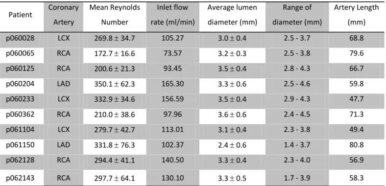
Patient Coronary Artery

Mean Reynolds Number

Inlet flow rate (ml/min)

Average lumen diameter (mm)

Range of diameter (mm)

Artery Length (mm) p060028 LCX 269.8  34.7 105.27 3.0  0.4 2.5 - 3.7 68.8 p060065 RCA 172.7  16.6 73.57 3.2  0.3 2.5 - 3.8 79.6 p060125 RCA 200.6  21.3 93.45 3.5  0.4 2.8 - 4.3 66.7 p060204 LAD 350.1  62.3 165.30 3.3  0.6 2.5 - 4.6 59.8 p060233 LCX 332.9  34.6 156.59 3.5  0.4 2.9 - 4.3 47.7 p060362 RCA 210.0  38.6 97.96 3.6  0.6 2.4 - 4.5 71.3 p061104 LCX 279.7  42.7 113.01 3.1  0.4 2.3 - 3.8 49.4 p061150 LAD 331.8  76.3 102.37 2.4  0.6 1.4 - 3.7 80.8 p062128 RCA 294.4  41.1 140.50 3.3  0.4 2.3 - 4.0 56.9 p062143 RCA 297.7  64.1 130.10 3.3  0.5 1.7 - 3.9 58.3

Table 3.1 - Patients, corresponding coronaries and some geometric and flow features of the ANGUS reconstructed vessels

3.1. Computational Fluid Dynamics

Computational fluid dynamics (CFD) simulations were executed thereafter, to

solve the Navier-Stokes equations (described in the Background chapter), which

(28)

Firstly, the discretization of the Navier-Stokes equations was executed by the

finite elements method (FEM). The geometries of the vessels were subdivided into

small cells (hexahedra) to form a mesh, by the finite element package Sepran (SEPRA

Analysis, Den Haag, The Netherlands). An example of the meshing of one

cross-section is shown in the left side of figure 3.1, while an example of the finite element

mesh of an entire coronary artery segment is shown in the right side of figure 3.1.

Figure 3.1 - Example of the finite element mesh of a coronary artery

Furthermore, in order to solve the Navier-Stokes equations (described in

Chapter 1.Background), it is necessary to prescribe both initial and boundary

conditions.

3.1.1. Assumptions and Boundary conditions

- No slip conditions at the walls: u(ux,uy,uz)=0;

- Rigid walls;

- Blood was modeled as an incompressible, homogenous and Newtonian;

(29)

Jorge Santos 29

Patients Pressure (Pa) Inflow rate (ml/min)

In Out Physiologic 50% 10% 1% p060028 464.02 -0.89 105.27 52.64 10.53 1.05 p060065 251.82 -0.13 73.57 36.79 7.36 0.74 p060125 178.99 -0.35 93.45 46.73 9.35 0.93 p060204 747.62 -0.66 165.30 82.65 16.53 1.65 p060233 288.74 -1.42 156.59 78.30 15.66 1.57 p060362 287.97 -0.85 97.96 48.98 9.80 0.98 p061104 407.31 -1.67 113.01 56.51 11.30 1.13 p061150 2518.70 -7.83 102.37 51.19 10.24 1.02 p062128 322.42 -0.31 140.50 70.25 14.05 1.41 p062143 828.96 -0.26 130.10 65.05 13.01 1.30

Average 629.66  697.00

-1.44  2.30

117.81  29.42

58.91  14.71

11.78  2.94

1.18  0.29

Table 3.2 - Inflow rate and pressure (in and out) values for the CFD calculations

3.2. Analysis

CFD calculations were performed for the three different geometries, according

to the ANGUS, QCA-3D and Straight 3D reconstruction method, of all ten vessels. The

output files from the CFD calculations, which contained information of the local SS,

flow velocity, pressure and geometry, were processed in MATLAB (Mathworks,

Natick, USA). The analysis of the calculations outcomes is hereby described.

3.2.1. ANGUS vs. Poiseuille

Primarily, the relationship between the average SS per cross-section based on

the CFD calculations and the lumen area were analyzed, and thereafter, the same

relationship was investigated using the SS based on the Poiseuille equation. The

average SS per cross section from the CFD calculations and the one based on

Poiseuille were then compared.

The next step was to analyze the influence of blood flow in the relationships

aforementioned. The input blood flow values in the CFD calculations were changed to

50%, 10% and 1% of the original (physiological) values, and new CFD calculations

were executed. Average SS and Poiseuille based SS, of the four different blood flow

values, were compared using regression analysis. In the Appendix is presented a table

(30)

Furthermore, Bland-Altman statistics were performed. Bland-Altman is a

statistical method that compares two measurement techniques [20]. In a

Bland-Altman plot, the x-axis stands for the average of the two techniques and the y-axis

stands for the difference between the two techniques. Horizontal lines were drawn at

the mean difference and at the limits of agreement, which were defined as the mean

difference plus or minus two times the standard deviation of the differences [21]. In

this case, the mean difference in average SS per cross section represents the

systematic error in average SS, and the regression line represents the proportional

error between techniques, meaning the error dependant on the mean magnitude of

the average SS.

In addition, a local wall SS histogram was built to visualize the local

distribution of both SS from the ANGUS method and Poiseuille based SS1.

Finally, the blood velocity profiles, from the four different blood flow values,

were analyzed. These cross-sections were located in specific regions of interest. Two

of them were located in a curved region and a highly stenotic region, respectively. For

the sake of comparison, the third cross-section, which was located in a “normal”

region (straight, and with low lumen area gradient), was analyzed.

All the results from these analyses are presented and described in Chapter 4.

3.2.2. ANGUS vs. Straight & ANGUS vs. QCA-3D

Since the analysis in these two chapters was similar, the methods used are

here described together.

In the first place, average SS per cross section and Lumen area plots for both

techniques were made, and compared. Then, the average SS from both methods

were compared using regression analysis. The correlation coefficients and the slope

and y-intercept values of the regression lines were registered.

Bland-Altman statistics and a local SS histogram, analogous to the ones

previously described, were also performed for both chapters.

(31)

Jorge Santos 31 The maximum SS value per cross section was also analysed, as well as the

longitudinal SS (exclusively in Chapter4. ANGUS vs. Straight).

Furthermore, high and low SS analyses were performed. These analyses were

performed per cross-section and per element (exclusively in Chapter 6 - ANGUS vs.

Straight). The low SS analyses, per element, consisted of locating the low SS elements

(<0.5 Pa) in both methods and calculate the percentage of elements that were

coincident (i.e. at the same location). The high SS analyses, per element, consisted of

locating the high SS elements in both methods and calculate the percentage of

coincident/overlapping elements. A high SS element was considered when the SS was

higher than the average SS per cross section plus the respective standard deviation (>





x Pa). A table with the threshold high SS values is presented in Chapter 5.

The high and low SS analyses per cross section were identical to the ones per

element. However, in this case, a high/low SS cross-section was counted when it

contained at least one element with high/low SS.

The sensitivity and specificity of the QCA-3D and Straight method when

predicting high or low SS elements (or cross-sections), comparing to ANGUS were

calculated. The sensitivity is a statistical measurement of the proportion of actual

positives which are correctly identified as such (e.g. the percentage of low SS

cross-sections determined by the QCA-3D or Straight method that are coincident with low

SS cross-sections determined by the gold standard ANGUS method). The specificity

measures the proportion of negatives which are correctly identified (e.g. the

percentage of non-low SS cross-sections determined by the QCA-3D or Straight

method that were also considered as non-low SS by the gold standard ANGUS

method.

The following table exemplifies how sensitivity and specificity were measured

for the calculation of low SS cross-sections. This procedure was analogous for the

(32)

ANGUS

Total cross-sections <0.5 Pa >0.5 Pa

QCA-3D

or

Straight

<0.5 Pa Overlapping

cross-sections (B) D - B

Low SS cross-sections from QCA-3D or Straight (D) >0.5 Pa C - B (A – D) – (C – B) A - D

Total cross-sections Low SS cross-sections

from ANGUS (C) A - C

Total cross-section of the vessel (A)

Sensitivity = B/C x 100% Specificity = ((A – D) – (C – B))/( A – C) x 100%

Table 3.3 – Measure of sensitivity and Specificity

The results from these analyses are presented and described in Chapter 5 and

Chapter 6.

3.2.3. Influence of geometric parameters

In Chapter 7 some geometric factors that are thought to be significant in the

SS calculations outcomes were analyzed. In the first place the lumen area gradient

was studied, which was compared with the average SS per cross section gradient, the

average SS and the local SS.

Additionally the curvature radius was analyzed, by comparing the curvature

radius and the Dean number with the maximum SS per cross section, using a

regression analysis.

As explained in section 3.2.1, the blood-flow was lowered to compare the

average SS based on ANGUS method and the Poiseuille equation based SS. The

lowering of the blood-flow reduces the presence of non-linearities in the average SS

vs. lumen area relationship. However these non-linearities do not disappear

completely. So, the presence of geometrical abnormalities in those specific regions

was investigated.

In the end, according to the factors previously studied, some guidelines with

(33)

Jorge Santos 33

Chapter 4. ANGUS vs. Poiseuille

One of the aims of this chapter was to prove the inverse relation between

average SS per cross section and the lumen area, by performing CFD calculations on

3D reconstructed geometries (from ANGUS) of real coronary arteries.

The main aim was to verify the relationship between the average wall SS

calculated by the finite element modeling and SS calculated by the Poiseuille

equation. Furthermore, the influences of blood flow in that relationship was tested.

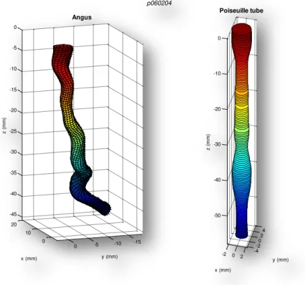
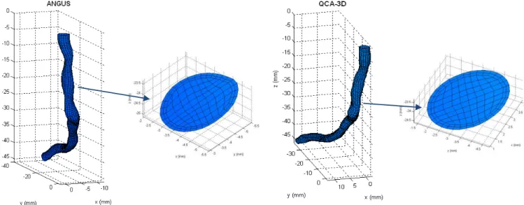
In figure 4.1, below, is represented an example of a left anterior descending

artery reconstructed by the ANGUS method (in the left) and a straight cylinder with

the same cross sectional area as the ANGUS one, which resembles a Poiseuille tube.

However, this tube has separated sections, which means that adjacent

cross-sections have no affect on each other.

Some geometrical and flow properties from the ten coronaries in study,

reconstructed by the ANGUS method, is available in the methods chapter.

Figure 4.1 - 3D reconstruction of a left anterior descending artery by the ANGUS method (in the left) and a Poiseuille cylinder with the same cross sectional area

0 10 20 -15 -10 -5 0 -45 -40 -35 -30 -25 -20 -15 -10 -5 0 y (mm) Angus x (mm) z ( m m )

-2 0 2

(34)

4.1. Results

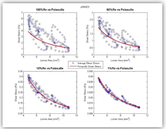
4.1.1. Average shear stress vs. Lumen area

The first question was whether it is accurate to determine the average SS in a

cross-section using the Poiseuille formula. Therefore, per cross-section, the average

SS was calculated, and compared with the SS based on the Poiseuille equation.

Figure 4.2 - Average SS vs. Lumen Area plots

Figure 4.2 shows the average SS vs. Lumen Area for four different arteries that

were randomly picked from the 10 studied arteries. It can be seen that the ASS over a

cross-section is inversely proportional to its area (see the bottom plots). Though, in

some patients this relation is not as linear as expected, like in the upper plots, where

the dots are more dispersed, and the inverse relationship is not so clear.

The following assignment was to calculate the average wall shear stress

according to the Hagen-Poiseuille’s equation: 4 ₃ R

Q

s _



(35)

Jorge Santos 35 (ml/min) and R is the cylindrical tube radius (m). The lumen radius was derived from

the lumen area. In order to put all the variables in S.I. units, the following equation

was used in MATLAB to calculate the shear stress: ₃

6 10 ) 6000 (

4

R Q

s

  

 



 

 . The

viscosity value used in this equation was 3.5 cP, which is an approximate value,

because the blood viscosity can differ a lot, depending on the hematocrit,

temperature and shear rate [22].

The Poiseuille SS values were plotted against the Lumen Area and then

superimposed on the Average SS vs. Lumen Area plots (example of four randomly

picked arteries is presented in figure 4.3).

Figure 4.3 - Average SS vs. Lumen Area, based on the CFD calculations (o) and the Poiseuille formula (

-

)

The plots above represent the average wall SS over a cross section calculated

by the finite element method (blue dots) and the wall shear stress calculated by the

Poiseuille equation (red line). It is observed that the blue dots are hardly equal, and

usually higher in value, to the SS values based on the Poiseuille equation. Hence, it is

(36)

probable cause for this is the geometric variability of the coronary vessels, since the

Poiseuille’s law only describes the flow in straight cylindrical tubes. In the appendix,

figure 11.1 displays analogous plots for all of the ten coronaries studied.

4.1.2. Influence of blood flow

The next question was how much the blood flow influences the relationship

between average SS and the lumen area. In order to investigate that, the input blood

flow rate values on the CFD simulations and in the Hagen-Poiseuille equation were

changed to 50%, 10% and 1% of the physiological values. Subsequently new Average

SS versus Lumen area plots were made.

By superimposing the Poiseuille based SS curve on these plots, the following

plots (figure 4.4) were obtained, which permit the comparison between calculated

average SS and Poiseuille SS for the different blood flows.

Figure 4.4 - Poiseuille shear stress versus Average shear stress – Influence of blood flow

The plot in the upper left side of the figure is the same that is shown at the

(37)

Jorge Santos 37 SS calculated by the Poiseuille equation (red line). By examining this plot it is seen

that the Poiseuille equation cannot accurately predict the wall SS of realistic coronary

arteries. However, when the blood flow rate is lowered (see the other three plots),

the average SS resemble the ones based on Poiseuille formula. This may happen

because when the flow rate is too low, geometric factors that can cause

non-linearities, such as curvature, torsion, sinuosity, among others, have much less

influence on the flow profile in the coronary arteries. However, even when the blood

flow rate is lowered to 1% of its physiological value there are some dots that don’t

follow the Poiseuille based line. The reason for this deviation from the Poiseuille

values will be discussed further in Chapter 7.

In addition, the Poiseuille SS was plotted versus the average SS based on CFD

calculation, in a scatter plot, with the intention of deriving the correlation coefficient

between them (figure 4.5).

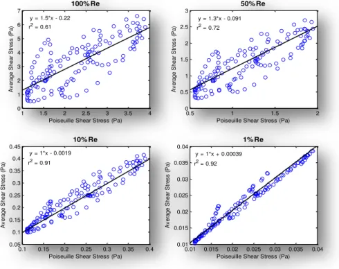
Figure 4.5 - Poiseuille and Average SS scatter plots for 100%, 50%, 10% and 1% of physiological blood flow

The correlation coefficient (r2) between the average SS and the Poiseuille SS is

presented in the table 4.1, below. A table with the regression line parameters is

available in the appendix (table 11.2).

0.01 0.015 0.02 0.025 0.03 0.035 0.04

Poiseuille Shear Stress (Pa)

A v e ra g e S h e a r S tr e s s ( P a ) 1% Re

y = 1*x + 0.00039

1 1.5 2 2.5 3 3.5 4

0 1 2 3 4 5 6 7

0.5 1 1.5 2

0 0.5 1 1.5 2 2.5 3

0.1 0.15 0.2 0.25 0.3 0.35 0.4

0.05 0.1 0.15 0.2 0.25 0.3 0.35 0.4 0.45

r2_{= 0.92}

y = 1.5*x - 0.22

r2_{= 0.61}

r2 = 0.72

y = 1*x - 0.0019

r2_{= 0.91}

(38)

Correlation coefficients (r2)

Patient 100%Re 50%Re 10%Re 1%Re p060028 0.61 0.72 0.91 0.92 p060065 0.59 0.68 0.80 0.83 p060125 0.61 0.76 0.93 0.94 p060204 0.52 0.61 0.86 0.94 p060233 0.67 0.74 0.86 0.86 p060362 0.80 0.84 0.93 0.95 p061104 0.61 0.71 0.90 0.94 p061150 0.68 0.73 0.90 0.97 p062128 0.61 0.67 0.88 0.98 p062143 0.81 0.89 0.90 0.99

Average 0.65  0.09 0.74  0.08 0.89  0.04 0.93  0.05

Table 4.1 - Correlation coefficients (r2)

Table 4.1 showed that, for every patient, the correlation between the average

SS and the Poiseuille based SS was increasing as the flow rate, or the Reynolds

number, became lower. The average r2 for the 100% Reynolds number was 0.65 

0.09 and for the 1% Reynolds number was 0.93  0.05, which was a significantly

different. The average r2 for the different blood flows was also presented in figure 4.6

as a bar plot.

100% Re 50% Re 10% Re 1% Re

0 0.1 0.2 0.3 0.4 0.5 0.6 0.7 0.8 0.9 1

Average r2

100% Re 50% Re 10% Re 1% Re

0 0.1 0.2 0.3 0.4 0.5 0.6 0.7 0.8 0.9 1

Average r2

Figure 4.6 - Average r2– Average SS vs. Poiseuille SS

4.1.3. Bland-Altman analysis

(39)

Jorge Santos 39 geometries, for the four different blood-flow percentages (100, 50, 10 and 1% of

physiological level). The Bland-Altman plot for the physiological Reynolds number is

presented next (figure 4.7).

Figure 4.7 - Bland-Altman plot (ANGUS vs Poiseuille)

The Bland-Altman analysis reveals that for all patients, and for 100% of the

physiological Reynolds number the average shear stress calculated from Poiseuille

underestimates the SS calculated from the CFD (from ANGUS) systematically by 1.43 

3.05 Pa, which is a significant error. The proportional error was also noteworthy

(Difference in SS = 0.79 x Average SS – 1.1), which means that the difference between methods gets larger as the average increases.

Reynolds Number Mean Difference ANGUS – Poiseuille (Pa)

b Average a

Difference   

a b

100% 1.43  3.05 0.79 -1.10 50% 0.32  0.99 0.55 -0.43 10% 0.13  0.088 0.23 -0.044

1% 7.6510-4  0.0047 0.12 -0.0022

Table 4.2 - Bland-Altman statistic results

In table 4.2 was presented the results of Bland-Altman statistics, and, as

expected, the systematic error got significantly lower (almost zero). Besides, the slope

of the regression line, which represents the proportional error, also decreased from

0.79 (at 100% Reynolds number) to 0.12 (at 1% Reynolds number); this means that

(40)

4.1.4. Local wall shear stress histogram

A local wall SS histogram was built (figure 4.8), to compare the local wall SS of

ANGUS with the SS calculated from the Poiseuille equation. Bars were created at 0.25

Pa intervals, resulting into 120 bars, in this case. The values from the ten patients

studied were included in the same histogram. A limitation of this analysis is that it

does not provide any information of the location of the SS values in the vessel.

Therefore geometrical information is lost.

The Poiseuille equation seems to give SS values lower than the SS derived

from the ANGUS method, since the number of elements at their peaks (both located

at relatively low SS values) is much higher for Poiseuille than for the ANGUS method.

The peak is situated in the 1 to 1.25 Pa interval, with 1693 elements in that wall SS

interval. While the Poiseuille peak is situated in the 1.25 to 1.5 Pa interval and has

4046 elements in that interval.

Taking in consideration that SS with values between 0 and 0.5 Pa is low SS and

SS with values >1.5 Pa is physiological shear stress and SS higher than the mean SS

plus one standard deviation (x = 3.88 + 5.50 Pa = 9.38 Pa) is high SS; for the

ANGUS vessels, the number of elements with low SS represent 7% of the total

number of elements, while 57% of the elements show physiological SS and 8% of the

elements exhibit high SS.

For the Poiseuille based SS,

there were no elements

with low SS (<0.5 Pa), while

the elements with

physiological SS represent

64% of the total number of

elements and only 2% of the

elements had high SS

values.

(41)

Jorge Santos 41 4.1.5. Velocity profiles

At some regions, with physiologic blood flow rate, the velocity profile per

cross-section exhibits an asymmetric distribution, which provokes asymmetric wall

shear stress. The patterns also demonstrate that the blood flow at physiological levels

is not Poiseuille like (parabolic distribution). However at low blood flow levels (10 and

1% of physiological) the velocity profile is parabolic. This, in combination to what is

seen at the lower two plots in figure 4.4, demonstrates that by lowering blood flow,

the calculated wall shear stresses are almost equal to the SS values based on the

Poiseuille formula.

Figure 4.9 represents a cross section that has a relatively large lumen area and

is located at a curved region of the artery. Consequently, the velocity profile (at

physiological and 50% Reynolds number) is asymmetric. The blood velocity is higher

near the outer side of the curvature and is lower at the inner side. However, at 10%

and 1% of the physiological Reynolds number, the velocity profile is reasonably close

to parabolic.

110th cross section

(42)

Furthermore, at some regions of the vessel where the lumen is narrowed, it is

observed that with physiological blood flow, the velocity profile is flattened. This

implicates that the wall SS at these sites is much higher than the corresponding SS

values based on Poiseuille parabolic flow. Figure 4.10 shows a cross section with a

small lumen area, which is located in a region where the lumen is gradually

narrowing. Therefore the velocity profile at physiological and 50% flow rate is

flattened, since the flow is probably turbulent. On the other hand at 10% and 1% flow

rate, the velocity profile is parabolic, as expected.

In addition, the table below presents, for the same cross section illustrated in

figure 4.10, the average SS from the CFD calculations, the Poiseuille SS and their ratio.

As seen in the table below, the difference between the average SS and the Poiseuille

SS, for 100% Reynolds number is 121% of the Poiseuille SS, while, for 1% Reynolds

number, it is only 7%. These values corroborate the fact that when the average SS is

much higher than the Poiseuille SS, the velocity profile in that cross section is

flattened. On the other side, when the average SS is similar to the Poiseuille SS, the

velocity profile is obviously parabolic.

Average SS from CFD calculations (Pa)

Poiseuille SS (Pa)

(Average SS – Poiseuille SS) / Poiseuille SS

100% Re 6.28 2.84 121%

50% Re 2.47 1.42 74%

10% Re 0.35 0.28 25%

1% Re 0.030 0.028 7%

Table 4.3 - Average SS from CFD calculations and Poiseuille SS for the 57th cross section of patient p060233. Re is an abbreviation for Reynolds number

Figure 4.11, below, shows the velocity profiles of a cross section in a region of

the vessel that is straight and has nearly constant radius. In this case, it is observed

that, even for physiological blood flow, the velocity profile is parabolic. This particular

cross section was chosen to serve as antagonism to the previous two examples,

because its average SS (for 100% Reynolds number) is almost the same as the

(43)

Jorge Santos 43

57th cross section

85th_{cross section}

Figure 4.10 - Velocity profiles for different blood flows (100%, 50%, 10% and 1%) for a stenotic cross section

(44)

Chapter 5. ANGUS vs. QCA-3D

The ANGUS technique, as described before, is a 3D reconstruction technique

based on the fusion of intravascular ultrasound (IVUS) and angiography, which

provide cross sectional and curvature information of the coronary arteries,

respectively. The QCA-3D is only based on multi planar angiography, so it only

provides accurate curvature information, lacking the exact cross sectional

information.

Therefore, the main aim of this chapter is to compare the SS based on the

QCA-3D reconstruction method with the SS based on ANGUS, and see how much

these differences between both methods influence the SS calculations outcome. So,

the CFD calculations described in the Methods chapter were repeated using the data

from the 3D reconstructions based on QCA-3D from the same vessel segments. The

CFD calculations made with the meshing from the QCA-3D method were performed

using analogous conditions used for the meshes from the ANGUS method, for each

similar vessel.

Some geometrical and flow properties from the ten coronaries in study,

reconstructed by the ANGUS method, is presented in the methods section. A similar

table (11.3) for the QCA-3D method is available in the Appendix. An example of a

coronary artery reconstructed by both these techniques is shown in figure 5.1,

located below.

The influence of geometric factors on the wall shear stress distribution in realistic human coronary arteries