On the interaction between financial constraints and economic growth

outubro 2019

João André Cimbron Cabral Mendes Jerónimo

On the interaction between financial

constraints and economic growth

Dissertação de Mestrado

Economia Monetária, Bancária e Financeira

Trabalho efetuado sob a orientação de

Professora Maria João Cabral Almeida Ribeiro Thompson

Professor José Assis Ribeiro de Azevedo

3

DECLARAÇÃO DE INTEGRIDADE

Declaro ter atuado com integridade na elaboração do presente trabalho académico e confirmo que não recorri à prática de plágio nem a qualquer forma de utilização indevida ou falsificação de informações ou resultados em nenhuma das etapas conducente à sua elaboração. Mais declaro que conheço e que respeitei o Código de Conduta Ética da Universidade do Minho.

Este é um trabalho académico que pode ser utilizado por terceiros desde que respeitadas as regras e boas práticas internacionalmente aceites, no que concerne aos direitos de autor e direitos conexos. Assim, o presente trabalho pode ser utilizado nos termos previstos na licença abaixo indicada. Caso o utilizador necessite de permissão para poder fazer um uso do trabalho em condições não previstas no licenciamento indicado, deverá contactar o autor, através do RepositóriUM da Universidade do Minho.

Atribuição CC BY

4

Resumo

Fricções financeiras constituem imperfeições nos mercados financeiros – por exemplo, mercados de crédito e de derivados - e, portanto, desvios dos quadros teóricos vigentes. Estas imperfeições constituem toda e qualquer situação passível de colocar um ou mais agentes económicos numa posição de vantagem comparativa em relação aos demais. Um exemplo recorrente de um tipo de fricções financeiras são as assimetrias de informação (Fu, 1996), que se podem manifestar de várias maneiras e, de acordo com a literatura empírica, ter vários tipos de repercussões. Com vista a contribuir para o corpo de literatura a ser produzido nesta área de investigação, e pela pertinência do tema à data da escrita desta dissertação, pretende-se construir um modelo teórico em que se estabeleça uma relação, na solução de equilíbrio da economia, entre um tipo específico de assimetrias de informação e o crescimento económico de longo prazo. No modelo proposto, o setor de bens de capitais opera num mercado monopolista, em que existem incentivos ao endividamento e posterior aquisição de patentes tecnológicas. Pretende-se ainda verificar a validade empírica do quadro teórico, com auxílio de estimadores Arellano-Bond (1998), aplicados em painéis dinâmicos.

5

Abstract

Financial frictions are imperfections observed in financial markets – e.g., credit and derivatives’ markets – and, therefore, deviations from the existing theoretical frameworks. These imperfections comprise every situation capable of putting some economic agent(s) in a position of advantage, relative to another(s). One common example of a type of financial frictions are informational asymmetries (Fu, 1996), that can express themselves in several way and, according to the empirical literature on the subject, have different kinds of consequences. With the purpose of contribute to the body of literature being produced in this research area, and by the relevance of this topic at the time of writing, we want to build a theoretical model in which we establish a relation between a particular kind of informational asymmetries and long term economic growth. In our proposed model, the capital goods’ sector operates in monopolistic competition, where there are incentives to indebtedness and consequent patents’ acquisition. We finally verify the empirical validity of our proposed theoretical framework with Arellano-Bond estimators (1998) applied to dynamic panels.

6

Content

2.2. On the financial sector: some relevant literature ... 20

2.3. BGG’s model ... 22

2.4. Some final considerations ... 26

3. Extending Romer’s model: an endogenous growth model with financial frictions ... 28

3.1. On the incompatibilities between the existing frameworks ... 28

3.2. The model ... 29

3.2.1. Balanced Growth Path Solution ... 37

3.3. Interaction between informational asymmetries and economic growth ... 40

3.4. Some final considerations ... 43

4. Testing the model: an empirical analysis ... 44

4.1. Data and Econometric Model ... 44

4.2.Interpretation and Discussion ... 51

5. Final Remarks ... 56

References ... 58

Appendix A ... 62

7

1. Introduction

With the latest financial crisis came the realization that finance’s impact on the real economy is definitely not innocuous. Not only have financial markets become greatly important for most developed countries, moving trillions of dollars on a daily basis, but they have also come to connect virtually all countries through increasingly complex and sophisticated instruments, thereby increasing the forms of liquidity available in the economy. Although these markets may present themselves as alternative sources of financing for traditionally bank-based economies such as the Eurozone, the ever-growing global interconnectedness carries some concerning drawbacks, such as important resource misallocations during the expansion phase of a financial cycle, and financial hyper-sensitivity due to increased systemic risk.

While one part of the existing literature already considers fluctuations in asset prices, credit and capital flows as some key factors of disturbance upon real macroeconomic variables (Claessens & Kose, 2018), another part does not acknowledge the role of financial frictions in the transmission of shocks through, e.g., asset prices, net worth, interest rates and/or monetary channels (Christiano, Eichenbaum, & Evans, 2005). The inexistence of consensus regarding the role of financial frictions in the real economy makes it hard to grasp and interpret in depth the whole economic reality. Reflecting this “academic and empirical controversy regarding the importance of financial channels” in the real economy (Gerke et al, 2012), most economic growth models do not contemplate financial frictions.

Jokivuolle and Tunaru (2017, pp. 1-7) do point out that every financial-economic crisis seems to be different from its predecessor, with no apparent regularity, although some specific types of asset, such as the real estate, appear to be more sensible to financial fluctuations. Nevertheless, crises can be interpreted, to some extent, as extreme manifestations of the existing relationship between the financial sector and the real economy (Claessens & Kose, 2013), which makes a strong call on economists to endeavor for a better understanding of macro-financial interactions. Plenty academic and policy literature has been produced in recent years on this topic. Even though there are still many questions unanswered, it is also true that some common denominators to financial dynamics have already been found. This claim is supported by the convergence of some key parameters used in policy models from institutions such as the Bundesbank, the European Central Bank, Banca d’Italia, Sveriges Riksbank and the National Bank of Poland (Gerke, et al., 2013).

8 It follows that Blanchard (2018), Borio (2018), Brunnermeier and Sannikov (2017), among others, regard existing theoretical models as no longer fully able to address current macroeconomic phenomena, specifically, that of the role of finance in the real economy. Notwithstanding, some notable advances have been made in recent years on this topic. Our work heavily relied on some significant studies such as Kiyotaki and More (1997) and, to a larger extent, Bernanke et al (1999). Wishing to contribute to this call for theoretical macroeconomic developments, we propose a growth model that contemplates financial frictions. This study explores the interactions between real growth variables and a particular kind of financial frictions that arises from informational asymmetries, within one economy, over an infinite horizon. Starting with a cost state verification problem, similarly to Morales (2003), we find the existence of a limit at which the existence of financial frictions appears to be irrelevant for economic growth, while the impact outside the neighborhood of this limit can either be negative or positive, depending on the possible marginal relations between an elasticity measure and growth.

We proceed as follows. In Section 2, we explain some of the literature’s and our model’s underlying roots and mechanics, with special emphasis on Romer’s model of endogenous growth (Evans, Honkapohja, & Romer, 1998), and the modelling of some types of financial frictions, with special emphasis on Bernanke, Gertler and Gilchrist (1999), hereafter referred as BGG. In particular, the choice of BGG as one of the underlying models has been made due to a perceived consensus in the literature regarding its importance in introducing and explaining financial frictions in dynamic economic modelling. In Section 3 we build our proposed model and proceed to find a balanced growth path solution and its main predictions. Here, we also focus on the main effects of informational asymmetries between the model’s agents on economic growth. Throughout section 4 we conduct an empirical analysis with dynamic panel data estimation methods, finishing with some concluding remarks in Section 5.

9

2. Literature Review

The matter of the determinants of economic growth and aggregate wealth distribution are key issues of macroeconomic studies and attempts to model these phenomena go far back. Solow (1956) developed a growth model based on physical capital accumulation with an exogenous household’s rate of savings, showing how long-run growth depends upon technical changes. Later, the Ramsey-Cass-Koopmans model endogenizes the saving rate, by deriving the evolution of capital stock from the interaction between maximizing firms and infinitely-lived households in competitive markets, thereby providing a check on Solow’s model, by showing that it survives once the analyst allows for more complex saving behavior. Both models build upon a one sector economy with a production function that takes as inputs 𝐾(𝑡) and 𝐴(𝑡)𝐿(𝑡), respectively, functions of capital and effective labor, the latter given by the labor function 𝐿(𝑡) and an effectiveness function 𝐴(𝑡) that proxies technological progress and, more precisely, a continuum of types of knowledge, ranging from the highly abstract to the highly applied. In both models, however, labor growth and technological progress are exogenous.

One could argue that the models that followed these studies were either based on human capital or technological progress as the main long-term growth determinants1. The first example of a

human capital-based macroeconomic growth model was developed by Lucas (1988). The author assumed a linear specification for the accumulation of human capital, which then allowed for endogenous growth. Earlier studies such as that of Becker (1964) helped the formulation of such theoretical models by drawing important macroeconomic implications from a microeconomic study of the links between education, output and overall economic performance. Despite the existence of a large body of literature on human capital-based growth models, we’ve chosen to support the endogenous growth on technological progress.

The case for the importance of technological progress – often measured as investment on research and development (R&D) - on economic growth is overwhelming. Perhaps one of the first relevant papers in doing so was that of Solow (1956), whose empirical work had as an important result the fact that accumulation of physical capital alone cannot account for most of the growth over time in the output per person – a very significant finding for the argument against the classical convergence hypothesis. Following works such as Arrow (1962), Phelps (1966) Evans et al (1998), Shell (2010)

1_{A third group of macroeconomic growth models, albeit less representative, eliminates the assumption of diminishing returns to capital in the}

10 made strong contributions for the current understanding of the role of technological progress in economic growth, suggesting that increases on the level of resources allocated to the R&D sector and consequent invention of new capital goods leads to a continuously increasing growth, through overall enhancements in terms of costs, output and resource allocation. The following subsection explains Romer’s model of endogenous growth in detail.

2.1. Romer’s model

The model of endogenous growth developed by George Evans, Seppo Honkapohja and Paul Romer (1998) comprises a set of properties that makes it utterly desirable to study and extend to the financial sector. First, the technology here is, to a large extent, endogenous2. This allows one to

fully analyze the system’s dynamics around the steady-state equilibria, regarding this unambiguously important variable. Second, building upon the rational expectations’ hypothesis, i.e., perfect-foresight, the model delivers multiplicity of equilibria in the (𝑔, 𝑟) space – common in Arrow-Debreu economies. This feature, and its extension by the introduction of expectational indeterminacy, delivers some convenient properties that characterize sequential economies, a framework often used to study the financial sector.

We start with a three-sector economy3 – final goods’, capital or intermediate goods’ and R&D

sectors. Labor is assumed to be fixed and positive in any moment in time. Furthermore, denoting 𝐿_𝐴(𝑡) as the function of labor devoted to R&D, and 𝐿_𝑌(𝑡) the function of labor devoted to the final goods’ sector, we’ll have that, in any moment in time, the existence of equilibrium in the labor market implies that

(2.1) 𝐿𝐴(𝑡) + 𝐿𝑌(𝑡) = 𝐿(𝑡)

The economy faces a Cobb-Douglas-like production function

2_{The authors design an output function of technology dependent on a parameter that reflects the incentives to R&D, which is formally exogenous.} 3_{The model’s derivation follows the works of Evans et al (1998), Thompson (2003) and Romer (2012).}

11 (2.2) 𝑌(𝑡) ∶= 𝐹(𝐿, 𝑥(. )) = 𝐿_𝑌(𝑡)1−𝛼(∫ 𝑥_𝑖(𝑡) 𝐴(𝑡) 0 𝑑𝑖) 𝛼

in which 𝐾(𝑡) = ∫₀𝐴(𝑡)𝑥_𝑖(𝑡)𝑑𝑖, which represents the capital at any given time, for 𝛼 ∈]0, 1[, 𝐴(𝑡), which is assumed to be continuous, represents the range of differentiated capital goods that have already been designed (proxy for technological progress and new ideas and designs), and

𝑥_𝑖(.) represents the number of units of capital of type i in use. The model, therefore, presents constant returns to scale, while 𝑥𝑖(.) presents diminishing returns to scale. However, given that

𝐴 is productive, technological growth compensates for the latter effect. Furthermore, it is assumed that the same production technology is used in all productive activities, i.e., (1) making consumption goods, (2) designs for new types of machines and (3) physical capital machines for types that have already been designed. Hence, the relative price of each output, given by the slope of the economy’s production possibility frontier, is linear.

The model also assumes an infinitely lived representative consumer that maximizes its discounted CRRA-like utility of future consumption 𝐶(𝑡)

(2.3) ∫ 𝑒−𝜌𝑡_{𝑢(𝐶(𝑡))𝑑𝑡} ∞ 0 , 𝑢(𝐶(𝑡)) =𝐶(𝑡) 1−𝜎 1 − 𝜎

subject to a budget constraint similar with that of the Ramsey-Crass-Koopmans model, where the present value of the lifetime consumption cannot exceed the consumer’s initial wealth plus the present value of his lifetime labor income, such that

(2.4) ∫ 𝑒−𝑟𝑡𝐶(𝑡)𝑑𝑡 ∞ 𝑡=0 ≤ 𝑋(0) + ∫ 𝑒−𝑟𝑡𝑤(𝑡)𝑑𝑡 ∞ 𝑡=0

12 from which results, by defining and calculating the Hamiltonian function, that the consumer faced with the constant rate of return 𝑟 will rationally choose to have his consumption growing at the rate given by the Euler equation

(2.5)

𝑔_𝐶 ∶=𝐶(𝑡)̇ 𝐶(𝑡) =

1

𝜎(𝑟 − 𝜌)

When dealing with time-varying production functions, one needs to address the matter of the inputs’ accumulation functions, i.e., the inputs’ production functions. Therefore, capital accumulation is given by

(2.6) 𝐾(𝑡)̇ = 𝑌(𝑡) − 𝐶(𝑡)

where the underlying assumption is that the real sector is always in equilibrium, that is, investment equals the private sector’s savings. This is an important observation to make, as it will follow us throughout the paper, being particularly relevant when analyzing the short-run capital structure model for the financial sector from Greenwald and Stiglitz (1993). Furthermore, given that the production function for new ideas is linear in the labor devoted to the R&D sector, and proportional to the existing stock of knowledge, its accumulation function is

(2.7) 𝐴(𝑡)̇ = 𝐵𝐿𝐴(𝑡)𝐴(𝑡)

where 𝐵 > 0 represents the efficiency of the research activities, and 𝐴(0) > 0. The linearity of 𝐴(𝑡)̇ in 𝐴(𝑡) implies the existence of a balanced growth path solution4. Knowledge interferes in

the production in two ways. First, a new design implies the production of a new capital good, which

4_{This is easily seen by solving the ordinary differential equation (2.7) for 𝐴(𝑡), from where we get that} 𝐴(𝑡) = 𝐴(0)𝑒∫ 𝐿0𝑡𝐴(𝜏)𝑑𝜏

13 will be, as I will soon explain, rented to the finalgoods’sector. Furthermore, it increases theexisting stock of knowledge, which constitutes a positive5 externality, given the non-rivalry property of

knowledge. This is the first important characteristic of knowledge that conveys important implications for the model. The other one is its partial excludability through patent laws, which is fundamental for the set of a monopolistic competition framework in the capital goods’ sector. Second, the higher the existing stock of knowledge 𝐴(𝑡), the higher the marginal productivity of researchers. This is a trivial consequence of the production function (2.2).

Unlike the capital goods’ sector, the final goods’ sector finds itself in a perfect competition environment. The latter rents capital goods at a rent 𝑅(𝑡) =𝑑𝑌(𝑡)

𝑑𝑥(𝑡) which it pays to the capital

goods’ sector which, in turn, faces the following supply curve6,

(2.8) 𝑅(𝑡) = 𝛼𝐿_𝑌1−𝛼𝑥(𝑡)𝛼−1

The problem lies, now, on how the capital goods sector, which operates in monopolistic competition, makes its production decisions. Assuming an unrestricted borrowing capacity at a fixed interest rate 𝑟, the monopolistic producers maximize their profits

(2.9) 𝜋(𝑡) = 𝑅(𝑡)𝑥(𝑡) − 𝑟𝑥(𝑡)

from where we, after taking the first order conditions, get the monopoly price

(2.10) _{𝑅 =} 𝑟

𝛼

5_{This is true because R&D firms are not required to compensate the researchers for past ideas. However, it is neglected by the authors, hence} creating a source of non-optimality of the final general-equilibrium solution, as it will be shown ahead.

6 _{The model enjoys the symmetry property, which means that 𝑥}

14 The background assumption that the developer of an idea has monopoly rights to the use of the idea implies that the developer can charge above the marginal production cost for the use of the idea. This generates profits that create incentives for R&D. The free-entry condition of the R&D sector implies that the present value of future discounted profits of selling the input embodying a new idea must, at least, equal the cost of creating. That is, the price of the initial investment is

(2.11) 𝑃_𝐴(𝑡) = ∫ 𝑒−𝑟(𝜏−𝑡)_{𝜋(𝜏)𝑑𝜏} ∞ 𝑡 = 𝑤(𝑡) 𝐵𝐴(𝑡)

where 𝑤(𝑡) represents the wage. By applying the Leibniz rule to its time differentiation, we get

(2.12) 𝑃_𝐴̇ (𝑡) = ∫ 𝑟𝑒−𝑟(𝜏−𝑡)_{𝜋(𝜏)𝑑𝜏} ∞ 𝑡 + [𝑒−𝑟(𝜏−𝑡)_𝜋(𝜏)] 𝑡 ∞ = 𝑟𝑃_𝐴(𝑡) − 𝜋(𝑡)

which Thompson (2003) interprets as being the trade-off that the companies face between investing the existing endowments at the risk-free return and investing on a patent and therefore opting for the risky monopoly rent returns, at any given time.

When we analyze the model’s long run dynamics, we are interested on a balanced growth path solution that, by (2.7), we know to exist. By observing that, on a balanced growth path, the rate of interest 𝑟 must be constant, we find, through (2.8), that the capital goods production

(2.13) 𝑥(𝑡) = 𝐿_𝑌(𝑡) [𝛼 2 𝑟 ] 1 1−𝛼

is also constant, giving that 𝐿_𝑌(𝑡) is fixed. This result consequently yields, by some substitutions in (2.2), that 𝐾 and 𝑌 grow at the same rate as 𝐴. Therefore,

15

(2.14) 𝑔𝑌 = 𝑔𝐾 = 𝑔𝐴

From which we can, by dividing (7) by 𝐴(𝑡), reach the technological progress growth mechanism

(2.15) 𝑔𝐴 = 𝐵𝐿𝐴(𝑡)

which implies that the growth rate of the technological progress depends on the number of researchers at any moment in time (assuming full employment of the production factor 𝐿). The assumption that the labor market is competitive implies that the wages are the same in every sector. Therefore, the intersection between the following equations

(2.16.1) 𝑤_𝑌 = 𝑑𝑌(𝑡) 𝑑𝐿𝑌(𝑡) = (1 − 𝛼) [𝐴𝑥 𝐿𝑌 ] 𝛼 (2.16.2) 𝑤𝐴 = 𝑑𝐴̇ 𝑑𝐿𝐴(𝑡) 𝑃𝐴 = 𝐵𝐴𝑃𝐴

yields the equilibrium price of investment in R&D

(2.17) 𝑃_𝐴 =1 − 𝛼 𝐵 [ 𝐴𝑥 𝐿_𝑌] 𝛼

16

(2.18) _{𝑟 =} 𝜋

𝑃𝐴

substituting in by the corresponding equations for the firms’ profits 𝜋(𝑡), (2.8) and (2.17), we get

(2.19) _𝑔

𝐴 = 𝐵𝐿̅ − 𝑟 𝛼

This important result can be extended, by working on the accumulation functions, hence concluding that the aggregate economy’s growth rate, under the perfect-foresight hypothesis, is given by

(2.20)

𝑔 = 𝛿𝛼𝐿̅ − 𝜌 𝛼 + 𝜎

The multiple equilibria appear when we introduce expectational indeterminacy in the model, under which changes in expectations cause the economy to switch between the high and low growth rate states, and when we combine complementarity effects between capital goods with a non-linear trade-off between investment and consumption. The first step is to define a state variable 𝑍

(2.21) 𝑍 = 𝑎𝐴(𝑡) + 𝐾(𝑡)

which comprises both physical capital and the patents. Hence,

17 Equation (2.22) characterizes a linear trade-off between consumption and investment. In order to introduce non-linearity (and, consequently, variability of the relative price of sectorial outputs), the authors create a convex cost function 𝜒(. ) such that

(2.23)

𝐶(𝑡) = 𝑦(𝑡) − 𝑍(𝑡)𝜒 (𝑍(𝑡 + 1) − 𝑍(𝑡) − 𝐷(𝑡)

𝑍(𝑡) )

in which 𝐷(𝑡) represents any depreciation of the physical capital stock. In order to later reach the BGP solution, the authors introduce the relative price of general capital 𝑍 given by7

(2.24) 𝑃_𝑍 = 𝜒′(𝑔_𝑍)

When considering equation (2.2), we realize that it implies that the capital goods are additively separable – therefore, independent. In order to introduce complementarity between capital goods, the authors specify

(2.25) 𝑦(𝑡) = 𝐿1−𝛼(∫ 𝑥(𝑡)𝛾 𝐴(𝑡) 0 𝑑𝑖) 𝜃

where 𝜃𝛾 = 𝛼, and 𝜃 > 1. If we assume that one unit of 𝑍 is required for the production each physical machine, we’ll have it distributed between machinery and new designs’ investment

7_{We take the limit, by ignoring the depreciation 𝐷(𝑡)}

𝑍(𝑡 + 1) − 𝑍(𝑡)

𝑍(𝑡) ≈

𝑍̇ 𝑍≡ 𝑔𝑍

18 (26) 𝑍(𝑡) = ∫ 𝑥𝑖(𝑡)𝑑𝑖 𝐴(𝑡) 0 + ∫ 𝑖𝜀𝑑𝑖 𝐴(𝑡) 0 = 𝐾(𝑡) + ∫ 𝑖𝜀𝑑𝑖 𝐴(𝑡) 0

in which 𝑖𝜀 _{represents the units of Z necessary for the production of the i-ith patent for a given}

capital good. To force the system to converge for a balanced growth path solution, the following restriction is made

(2.27)

𝜀 =𝜃 − 1 1 − 𝛼

which the authors have obtained through numerical methods. Similar assumptions of those made for solving the model without capital goods’ complementarities nor non-linear trade-off between investment and consumption lead to the multi-equilibria solution. The profit maximizing capital goods’ sector sets the monopolistic rent equal to their inputs’ marginal productivity

(2.28) 𝑅(𝑡) = 𝑑𝑦(𝑡) 𝑑𝑥(𝑡)= 𝜃𝛾𝐿 1−𝛼_𝑥(𝑡)𝛾−1_{(∫ 𝑥(𝑡)}𝛾 𝐴(𝑡) 0 𝑑𝑖) 𝜃−1

Now, the monopolistic firm maximizes it revenues 𝑅(𝑡)𝑥(𝑡), with respect to its expenditures 𝑟𝑃_𝑍𝑥(𝑡). The first order condition yields that

(2.29)

𝑅 =𝑟𝑃𝑍 𝛾

which enables us to, through the model’s symmetry properties, solve the problem for its balanced growth path, from where we get

19

(2.30) 𝑔𝑍 = 𝑔𝐾 = 𝑔𝑌 = (1 + 𝜀)𝑔𝐴

The key to determine 𝑔_𝐴 is to impose the non-transversality condition that arises from the Fisher equation on 𝐴(𝑡), such that

(2.31)

𝑃_𝑍𝐴(𝑡)𝜀 _{= ∫ 𝑒}−𝑟(𝜏−𝑡)_{𝜋(𝜏)𝑑𝜏} ∞

𝑡

which, by time-differentiating, with 𝑃_𝑍 held constant, gives

(2.32) 𝑔𝐴 = 1 𝜀(𝑟 − 𝜋 𝑃_𝑍𝐴(𝑡)𝜀)

We can reduce (2.32) by one degree of uncertainty by transforming the equation so it becomes dependent on the behavioral parameter 𝛼. This equation then delivers the new growth curve, given by a more complex form that generalizes (2.20). In any macroeconomics setting, whenever there are multi-equilibria, we have learned to accept that they have different degrees of stability. The concept of stability relates with the idea that, for a given set of initial values for the state variable, the system’s dynamic behavior will make it fluctuate between equilibriums. In particular, (2.32) provides us a multiple equilibrium framework, which will fluctuate between the high and low growth solutions, depending on time-specific phenomena and preferences. Therefore, the authors introduced the stability under learning criterium, implying that the agents will learn and react to the variables’ values at any given time, according to the following rule

(2.33)

𝑟(𝑡 + 1)𝑒 = 𝑟(𝑡)𝑒+ 𝛿(𝑡)(𝑟(𝑡) − 𝑟(𝑡)𝑒), 𝛿(𝑡) = 𝛿 𝑡

20 hence generating a dynamic interest rate that tells us how the equilibria fluctuate. Under this framework, agents base their consumption/investment choices on expected values for the future interest rate, 𝑟𝑒_{, which will, in turn, affect the aggregate growth rate. This aggregate growth rate}

is, in turn, considered on the firms’ production decisions, which require a sufficient amount of financial aid, which is dependent on the realization of the interest rate. This generates growth cycles, providing the existence of a dynamic rate of interest.

2.2. On the financial sector: some relevant literature

What the previous section fails to contemplate is the possibility of agent-based disturbance factors. These appear in the literature in many ways, such as intermediary rates and capital flows, or any type of information asymmetries. Their effects on financial markets are, however, controversial. Trivedi (2015) finds, by analyzing financial innovation8 on the Indian banking system, a positive

relation between innovation and enhanced bank performance, measured in terms of profitability and stability of the income. Similar conclusions regarding the beneficial effects of innovation are found in Guimaraes et al (2010), for whom it comprises dimensions such as strategic leadership, competitive intelligence, management of technology and some specific characteristics of the bank or firm’s change process used to conduct innovation projects. However, Epure and Lafuente (2015), by analyzing the Costa Rican banking sector, argue that, although the general average bank-specific inefficiency has decreased in the pre-2008 period, characterized by increased innovation practices, no such relation was observed during the post-crisis period, during which the average banking specific inefficiency scores from the authors’ technology concept, and the average return on assets and net interest margin all remained relatively unchanged. This second period faced a significant increase on the regulatory pressure, therefore jeopardizing innovative impulses and practices, on a global scale. Therefore, at least at a micro level, it may be reasonable to assume that the effects of financial frictions on economic performance aren’t all straightforward.

In a frictionless economy, funds can flow to the most profitable project, and such flows are determined by differences in productivity and risk aversion at the micro level, and differences in

8_{The author studies financial innovation as being foremost, but not exclusively, the search for development of new income sources and consequent} increases in portfolio diversification, at the bank-level. These include, e.g., non-loan related fees.

21 capital and labor at the macro level (Brunnermeier, Eisenbach, & Sannikov, 2013). In an economy with financial frictions, however, there is an inherent instability and the agent dynamics are utterly probabilistic, due to the existence of uncertainty. Hall (2013) suggests that such frictions can be thought of as a spread between the returns earned in businesses from the physical capital – plant and equipment – and the returns earned by savers, or the market cost of capital. This could suggest that the uncertainty sources of an economy are non-negligible for the purposes of economic and policy analysis. The accumulation of such frictions prevents funds from flowing to undercapitalized sectors, hence preventing Pareto-optimality, through resource misallocations, and generating unequal growth and development opportunities.

The dynamics of economies with financial frictions are highly non-linear9 (Brunnermeier & Sannikov,

2017), which is why small shocks can lead to significant economic dislocations10. This was the

case of the Lehman Brothers’ collapse in September 2008, which triggered a self-sustained sequence of balance-sheet defaults that spread worldwide. Brunnermeier and Sannikov point out that, while the financial markets are self-stabilizing in normal times, economies become quite vulnerable to a crisis after a run up of debt imbalances and credit bubbles. Greenwald and Stiglitz (1993) developed a simple model of economic fluctuations, that comprises some of the key issues that characterize the financial sector’s short-run dynamics, based upon the kinds of informational imperfections that are chiefly related to adverse selection and moral hazard.

There is a significant number of other models that assume various financing restrictions. Specifically, we can identify two main approaches of financial frictions in macroeconomics. The first approach is due to Kiyotaki and Moore (1997), which focuses on the idea of the inalienability of human capital. The assumption results in the lenders’ demand that the value of the borrowers’ durable assets must at least equal the value of the outstanding debt. Hence, these assets play a dual role – they are both means of production and serve as collateral for current loans. The second approach is that of BGG (1999). Despite the similarities between the approaches, such as the need of an optimal contract between the lender and the borrower as a solution to an agency problem and the feedback effects from asset markets, they are quite different. Essentially, BGG build upon a debt contract as a solution to a problem of asymmetric information between the lender and the borrower, which endogenously motivates the existence of an external financing premium. Later

9_{The very nature of these dynamics makes the system’s behavior inherently probabilistic.}

10_{The most important features of such shocks are their persistence, which refers to its duration in time, and amplification, which refers to its ability} to spread and reproduce its effects along a growing number of agents and economies.

22 models such as that of Morales (2003) build upon the same agency problem as in BGG, albeit in a fashion different from the standard sticky price DSGE framework. The following subsection explains the partial equilibrium framework of BGG, in the context of the authors’ log-linearized stochastic model.

2.3. BGG’s model

BGG give us two reasons for the introduction of financial frictions in macroeconomic models. First, doing so seems to enhance the models’ capacity of explaining cyclical fluctuations, such as credit supply in the economy. Second, a lot of empirical research on the determinants of aggregate supply and demand attributes an important role to financial frictions. Thus, the authors developed a variant of the dynamic new keynesian framework – i.e. stochastic aggregate growth that incorporates monetary policy, monopolistic competition and nominal price rigidity -, modified to allow for financial accelerator effects on investment. Their main purpose is to assess how credit market frictions influence the monetary policy transmission mechanisms.

The model comprises three kinds of agents: households, retailers and entrepreneurs. Similarly to Romer’s model, households are assumed to be infinitely lived. Furthermore, they hold the economy’s goods, services and interest bearing assets. Retailers are, together with entrepreneurs, market suppliers, and are assumed to work in monopolistic competition in order to introduce price stickiness in the model. This ensures a linear relation between the demand for capital goods and the net worth of this model’s most important agent.

Entrepreneurs have, indeed, a central role in BGG’s framework. Each single entrepreneur is finitely lived, with a constant probability 𝑃 ∈ [0,1] of surviving until the following period. At any given moment 𝑡, each entrepreneur buys physical capital, financed by their current net worth and external funds, combined with labor to generate output in 𝑡 + 1. The external funds thus finance the difference between input costs and the entrepreneur’s net worth, such that

(2.35) _𝐵𝑡+1𝑗

23 where 𝐵_𝑡+1𝑗 _{represents the debt amount that the 𝑗-th entrepreneur must incur in at 𝑡 + 1, 𝑄}

𝑡 the

price of capital goods at 𝑡, 𝐾_𝑡+1𝑗 _{the amount of capital goods purchased for use at 𝑡 + 1 and 𝑁} 𝑡+1

𝑗

its net worth at the end of 𝑡, going to 𝑡 + 1.

Building upon Townsend (1979) the authors introduced a cost state verification problem in order to endogenously motivate the existence of an external finance premium, which will depend on the borrower’s financial position at 𝑡 + 1. The nature of this problem implies that the entrepreneur holds more information than the lender, regarding its future net worth, to the extent that he can observe its capital returns at 𝑡 + 1. This means that there’s asymmetric information regarding the borrower’s ability to repay its loan at 𝑡 + 1, resulting in the need of an optimal contract to mitigate the risk of adverse selection and moral hazard. The optimal contract established between the lender and the borrower is characterized by the minimum requirement rule for external financing

(2.36) _𝑤̅𝑗_𝛾

𝑡+1𝑄𝑡𝐾𝑡+1 = 𝑍𝑡+1 𝑗

𝐵_𝑡+1𝑗

where 𝑍_𝑡+1𝑗 _{represents a gross non-default rate, 𝑤}

̅𝑗 the limit value of the idiosyncratic shock 𝑤𝑗 and 𝛾_𝑡+1 represents the aggregate risk of the economy. Both 𝑤𝑗 _{and 𝛾}

𝑡+1 are stochastic

variables. Upon the borrower’s net worth realization at 𝑡 + 1, one of two situations may occur. If 𝑤𝑗 _{≥ 𝑤̅}𝑗_{, the borrower is able to repay the loan at the rate 𝑍}

𝑡+1

𝑗 _{to the financial intermediary. If,}

however, 𝑤𝑗 _{< 𝑤̅}𝑗_{, the borrower goes bankrupt. This means that the intermediary incurs in an}

auditing cost ℎ𝑤𝛾_𝑡+1𝑄_𝑡𝐾_𝑡+1 and keeps what he finds, while the defaulting entrepreneur receives nothing. Given the finite cardinality of the relevant set of nature states of 𝑤𝑗 _{at any given moment,}

and assuming that the intermediary is able to diversify its portfolio, the loan contract satisfies

(2.37) {[1 − 𝐹(𝑤̅𝑗_)]𝑤̅𝑗 _{+ (1 − ℎ) ∫ 𝑤𝑑𝐹(𝑤)} 𝑤̅𝑗 0 } 𝛾_𝑡+1𝑘 _𝑄 𝑡𝐾𝑡+1 𝑗 = 𝑟_𝑡+1(𝑄_𝑡𝐾_𝑡+1𝑗 − 𝑁_𝑡+1𝑗 )

24 where 𝑟𝑡+1 represents the riskless rate at 𝑡 + 1. This way, we are able the express the lender’s

expect return as a function of the cutoff value of the idiosyncratic shock 𝑤̅𝑗 _{on the entrepreneur’s}

productivity. Once we’ve determined the value for 𝑤̅𝑗, contingent upon the ex post realization of the systemic shock 𝛾_𝑡+1𝑘 _{and the ex ante choices of 𝑄}

𝑡𝐾𝑡+1 𝑗 _{and 𝐵}

𝑡+1

𝑗 _{, we now address the}

entrepreneur’s optimal choice of 𝐾_𝑡+1𝑗 _{. By making expectations regarding the realization of 𝛾} 𝑡+1𝑘 ,

the entrepreneur maximizes

(2.38) 𝐸 {[1 − ℎ ∫ 𝑤𝑑𝐹(𝑤) 𝑤̅𝑗 0 ] 𝑈_𝑡+1𝑟𝑘 } 𝐸{𝛾_𝑡+1𝑘 }𝑄_𝑡𝐾_𝑡+1𝑗 − 𝑟_𝑡+1(𝑄_𝑡𝐾_𝑡+1𝑗 − 𝑁_𝑡+1𝑗 ) subject to (2.37), where 𝑈_𝑡+1𝑟𝑘 _≡ 𝛾𝑡+1𝑘

𝐸{𝛾_𝑡+1𝑘 }. The external finance premium is thus derived from the

monitoring costs, which the entrepreneur internalizes due to the assumption that he is risk neutral. The maximization of (2.38) relative to 𝐾_𝑡+1𝑗 _{and 𝑤}

̅𝑗 _{yields the following relation for optimal capital}

purchases: (2.39) _𝑄𝑡𝐾 𝑡+1 𝑗 = 𝜑(𝑠𝑡)𝑁𝑡+1 𝑗 , 𝑤𝑖𝑡ℎ 𝜑(1) = 1, 𝜑′(. ) > 0 where 𝑠_𝑡≡ 𝐸 {𝛾𝑡+1𝑘

𝑟𝑡+1} represents the expected discounted return to capital. This means that the

higher the expected capital returns relative to the riskless rate – i.e. the loan repayment’s rate minus the premium – the higher the capital investment and, consequently, the higher the indebtedness. There is also a multiplicative effect of the entrepreneur’s net worth on capital acquisition. Therefore, the higher the financial stability, the larger the credit and the capital investment. Furthermore, this implicitly means that the higher the expected discounted return, the lower the expected default probability.

This partial equilibrium is integrated within a broader framework. The authors specify an Romer’s-like aggregate production function for any 𝑡 given by

25

(2.40) 𝑌_𝑡 = 𝐴_𝑡𝐾_𝑡𝛼_𝐿 𝑡 1−𝛼

where 𝑌_𝑡 represents the aggregate output of wholesale goods, 𝐾_𝑡 the aggregate amount of capital purchased by entrepreneurs in period 𝑡 − 1 , 𝐿𝑡 the labor input and 𝐴𝑡 is an exogenous

technological parameter. The discrete accumulation function for the aggregate capital purchases is given by (2.41) 𝐾𝑡+1 = 𝜃 ( 𝐼_𝑡 𝐾𝑡 ) 𝐾𝑡 + (1 − 𝛿)𝐾𝑡, 𝜃(0) = 0, 𝜃′(. ) > 0

where 𝐼_𝑡 represents the aggregate investment expenditures and 𝛿 the depreciation rate. The inclusion of adjustment costs results in a variable price of capital, making price variability contribute to volatility in entrepreneurial net worth, which the authors define by

(2.42) 𝑁_𝑡+1 = 𝑃𝑉_𝑡+ 𝑊_𝑡𝑒 where (2.43) 𝑉_𝑡 = 𝛾_𝑡𝑘_𝑄 𝑡−1𝐾𝑡 − (𝑟𝑡+ ℎ ∫ 𝑤𝛾_𝑡𝑘𝑄𝑡−1𝐾𝑡 𝑑𝐹(𝑤) 𝑤̅𝑗 0 𝑄𝑡−1𝐾𝑡 − 𝑁𝑡−1 ) (𝑄𝑡−1𝐾𝑡 − 𝑁𝑡−1)

represents the entrepreneurial equity and 𝑊_𝑡𝑒 _{denotes the entrepreneurial wage}11. By further

specifying the total labor input as

11_{The authors assume that, besides their net worth and external funds, entrepreneurs finance their current period’s production through the inelastic} supply of one unit of labor to the labor market.

26

(2.44) 𝐿𝑡 = 𝐻𝑡Ω(𝐻𝑡𝑒)1−Ω

where Ω ∈]0,1[, the authors obtained the demand curves for household and entrepreneurial

labor, through which they deduced the aggregate entrepreneurial net worth

(2.45) 𝑁𝑡+1= 𝑃 [𝛾𝑡𝑘𝑄𝑡−1𝐾𝑡 − (𝑟𝑡+ ℎ ∫ 𝑤𝛾𝑡𝑘𝑄𝑡−1𝐾𝑡 𝑑𝐹(𝑤) 𝑤̅𝑗 0 𝑄𝑡−1𝐾𝑡 − 𝑁𝑡−1 ) (𝑄𝑡−1𝐾𝑡 − 𝑁𝑡−1)] + (1 − 𝛼)(1 − Ω)𝐴𝑡𝐾𝑡𝛼𝐻𝑡 (1−𝛼)Ω

Equation (2.45) thus describes the endogenous variation in the aggregate net worth, whilst the aggregate form of (2.39) describes how financial strength and expectations regarding future systemic shocks influence the cost of capital. After introducing household, retail and government sectors, the authors obtained the full model through regular Taylor approximations of the stochastic factors. The final set of log-linearized equations allows the researcher to assess the monetary policy transmission mechanisms in a macroeconomic environment with financial frictions.

2.4. Some final considerations

This section comprised some theoretical examples from the fields of economic growth and finance and was meant to explore the possibility of synergy between the two. Although some of the most relevant endogenous growth models don’t necessarily comprise agent-based financial frictions, some partial equilibrium frameworks have appeared in the literature to meet this area of research potential. Despite a perceived consensus in the literature regarding the relative importance of studies such as BGG (1999) and Kiyotaki and Moore (1997), others have managed to introduce different financial factors within more conventional frameworks. Greenwald and Stiglitz (1993), from a two-agent labor-dependent economy with risk averse firms, built a general price level which fluctuates according to a marginal bankruptcy cost. Similarly to BGG, firms make decisions according to an equation that reflects their solvency situation. By construction, they show that the

27 representative firm’s profit maximizing output is a linear function of their equity. Others, like Pietra and Siconolfi (1996), characterize the economy’s equilibrium as the representative household’s maximization problem, which depends on expectations about future realizations of stochastic variables – namely, the asset prices according to which their portfolio allocations vary. By representing the economy as a space of real open subsets representing the households’ utility functions, the authors represented the equilibrium price solution as a smooth manifold diffeomorphic to the space in which all states of nature are embedded. Hernández and Santos (1996) follow a similar methodology.

Given the in-depth analysis of Romer and BGG’s models, the following section will proceed to integrate some of the mechanisms. There are a few factors that motivated the choice of the latter in the proposed expansion. First, in both models we find three productive sectors, with at least one working in monopolistic competition. Second, in both models we find a retailer – albeit with different designations – and an intermediate goods sector whose production inputs are capital goods. These factors hint at a similar architecture base between the two models, which may suggest a possible complementarity between them.

28

3. Extending Romer’s model: an endogenous growth model with

financial frictions

In this section, we proceed as follows. First, we address some of the technical incompatibilities between Romer’s model and BGG’s partial equilibrium framework. The purpose is to help understand the specific challenges that one needs to face if we ought to create a full general equilibrium model with financial frictions. Second, we start building Romer’s model with our proposed modifications, whilst explaining why we believe they can be implemented. Third, we deduce the economy’s balanced growth path solution. Fourth, we analyze the transition dynamics of the expanded model, followed by some concluding remarks.

3.1. On the incompatibilities between the existing frameworks

We start by addressing the perfect-foresight hypothesis. Under BGG (1999), this does not hold, given that the entrepreneur’s net worth at 𝑡 + 1 is uncertain, subject to a decomposed risk measure which captures both the aggregate and the idiosyncratic risk. The uncertainty around the net worth’s realization (which we proxy by the capital firms’ profit functions) gives rise to an informational asymmetry between the lender and the borrower which, in turn, gives an endogenously motivated reason for the existence of an external finance premium within BGG, whose existence is meant to compensate the lender for a problem of adverse selection and moral hazard12. The asymmetry constitutes a financial friction that can lead to more pronounced

macroeconomic fluctuations, through BGG’s financial accelerator (Claessens & Kose, 2018, pp. 75-79). We would then argue that Romer’s deterministic setting constitutes a problem for the introduction of these financial imperfections.

Unlike the infinitely lived agents in Romer, the entrepreneurs in BGG are allowed to go bankrupt, should the cut-off value of the following period’s capital returns be belowthe outstanding debt value multiplied by the risk-free rate of the economy. This is the external finance rule that borrowers must meet at each moment in time, in order to get externalfinancing at 𝑡 andcontinue theproduction,

12_{The existence of uncertainty around the net worth’s realization and the drawing of an optimal contract as a solution to an agency problem is also} present in KM and other studies like Carlstrom and Fuerst (1997), who integrates collateral constraints on the firm’s side by assuming that labor employment must be partially financed through loans.

29 at least, until 𝑡 + 1. The idiosyncratic nature of the entrepreneurs’ bankruptcies holds the authors from assuming symmetry within their model, hence studying the partial equilibrium in terms of individual agents at arbitrary moments in time, in contrast with what happens in Romer’s framework. Given that macro-financial linkages originate at the microeconomic level, one would expect for any model with financial frictions to shed light over agent-based phenomena. However, given the very nature of the field, we ought to analyze aggregate dynamics and patterns. Therefore, under the integration of BGG’s partial equilibrium within a R&D-based endogenous growth framework, the agents’ finite horizons may be a concern.

So far, we’ve identified three incompatibilities between BGG’s partial equilibrium and Romer’s model: the latter is fundamentally deterministic, while BGG has a probabilistic setting; in the two models, agents present different time horizons; and, while Romer’s framework is derived in continuous time, BGG is written in discrete time, as suggested by the above mentioned one-period gap between the economic decision and the stochastic net worth’s realization. Our main purpose is to expand Romer’s model, so as to encompass BGG’s partial equilibrium. In the following section, we propose ways to surpass these incompatibilities, in order to build a complete general equilibrium model of endogenous growth with financial frictions.

3.2. The model

Let’s take the partial equilibrium setting of external finance dynamics in BGG, where the authors start by stating that

(3.1) _𝐵 𝑡+1 𝑗 = 𝑄𝑡𝐾𝑡+1 𝑗 − 𝑁_𝑡+1𝑗

where 𝐾_𝑡+1𝑗 _{represents the capital bought at 𝑡 by the 𝑗 -th entrepreneur, 𝑄} 𝑡𝐾𝑡+1

𝑗 _{the payoff}

realized at 𝑡 + 1, 𝑁_𝑡+1𝑗 _{the net worth of the 𝑗-th entrepreneur, realized at 𝑡 + 1, and 𝐵} 𝑡+1

𝑗 _{is the}

debt amount needed by the 𝑗-th entrepreneur at 𝑡 + 1, borrowed from a financial intermediary (e.g. a bank). This means that, at each period, each entrepreneur acquires physical capital through

30 his personal net worth and loans, which is combined with labor through some production technology to generate output in the following period.

In order for the entrepreneur’s net worth to influence the loan terms, the borrowers need to face finite time horizons. The rationale is pretty straight forward: the assumption of a Cost State Verification (CSV) problem in BGG gives an endogenously motivated reason for the existence of an external finance premium, i.e., an opportunity cost for internal funding, meant to compensate the lender for a problem of adverse selection and moral hazard. This premium will depend on the borrower’s ability to repay its loan at 𝑡 + 1 – i.e., its net worth –, which will be dependent on a default probability. For such a probability to exist, the entrepreneur must be allowed to go bankrupt, hence the purpose of the finite horizon, which captures the phenomenon of the continuous “birth” and “death” of firms, within a given economy.

We want the entrepreneurial sector in BGG to be analogous to Romer’s capital sector. There are two difficulties that we need to surpass. The first one is the extension of the partial equilibrium to a continuous framework, which implies reducing the one-period gap to an arbitrarily small gap between the agents’ decisions and the variables’ realization. Second, the entrepreneur’s finite horizon is incompatible with Romer’s framework, in which firms don’t go bankrupt. This constitutes a problem if we ought to integrate the financial accelerator mechanism. The problem of expanding Romer’s model such as to encompass BGG’s partial financial equilibrium is, we believe, intimately related with the solution of the two above mentioned incompatibilities13.

By looking at equation (3.1), one could argue that a continuous approximation would be fairly straight forward, given that 𝐵_𝑡+1𝑗 _{is linear both in 𝑄}

𝑡𝐾𝑡+1

𝑗 _{and in 𝑁} 𝑡+1

𝑗 _{. However, despite the}

mathematical validity, this approximation by time-differentiation wouldn’t be economically reasonable. To understand why, let us rewrite (3.1)

(3.2) _𝐵 𝑡+ℎ 𝑗 = 𝑄𝑡𝐾𝑡+ℎ 𝑗 − 𝑁_𝑡+ℎ𝑗

13_{The original authors introduced monopolistic competition in the retail sector so as to obtain nominal rigidity, intrinsic to the Dynamic New} Keynesian approach, suited for their purpose of monetary policy analysis. A monopolistic entrepreneurial sector would imply a non-linear relation between the entrepreneur’s net worth and his demand for capital. We believe that, by proxying the capital sector’s net worth by the profit function, the problem of a non-linear relation does not arise here.

31 with respect to an arbitrarily small time amount ℎ. When ℎ → 0, (3.2) implies that the borrower both receives and repays the external funds almost instantaneously, which not only is unintuitive, as it does not represent the reality of credit flows at the firm level.

We know that the free entry condition in Romer’s capital market implies that the investor needs to make an initial investment 𝑃𝐴(𝑡) to participate. If we assume that this initial cost is financed

through a loan, in a similar fashion of Carlstrom and Fuerst (1997) with the labor employment, we can introduce a model of debt management to replace the current loan dynamics present in BGG. We do this by stating that, in any given period, the firm pays some percentage of the outstanding debt, which corresponds to the initial investment cost 𝑃_𝐴(𝑡).14 The rationale is that some net losses

are expected at the beginning of the firm’s creation, which may turn to profits once it becomes fully developed. In order to preserve the aggregate capital accumulation, we introduce the following transversality condition (3.3) ∫ (𝑃𝐴(𝜏) − 𝛽(𝜏)𝑃𝐴(𝜏))𝑑𝜏 𝑡 0 = 0

where 𝛽(𝜏) > 0 represents a variable portion of outstanding debt paid at each moment in time. The condition implies the full repayment of outstanding debt, in the long run.

This is an important step in the model’s architecture. The optimal contract established between the lender and the borrower in BGG is characterized by the minimum requirement rule for external financing

(3.4) _𝑤̅𝑗_𝛾

𝑡+1𝑄𝑡𝐾𝑡+1 = 𝑍𝑡+1 𝑗

𝐵_𝑡+1𝑗

where 𝑍_𝑡+1𝑗 _{represents a gross non-default rate, 𝑤}

̅𝑗 the limit value of the idiosyncratic shock given by the stochastic variable 𝑤𝑗_{, which fluctuates in the interval [0,1], such that 𝑤}𝑗 _{≥ 𝑤̅}𝑗 _implies

that the lender is able to repay the loan at the rate 𝑍_𝑡+1𝑗 _{, and 𝛾}

𝑡+1 represents the aggregate risk

14_{Further in this study, we show how this introduction of indebtedness comes at the cost of the complementarities between capital goods} assumption.

32 of the economy. If, on the other hand, 𝑤𝑗 _{< 𝑤̅}𝑗_{, then the firm is unable to repay its loan and goes}

bankrupt. Under the proposed model of continuous debt management, we can adapt (3.4) to our capital sector

(3.5) 𝑤̅_𝑗𝛾𝑅_𝑗(𝑡)𝑥_𝑗(𝑡) = 𝑟𝑥_𝑗(𝑡) + 𝑍_𝑗(𝑡)𝛽_𝑗(𝑡)𝑃_𝐴,𝑗(𝑡)

where 𝑅_𝑗(𝑡) represents the 𝑗-th firm’s selling price of its capital goods 𝑥_𝑗(𝑡), and 𝑟 represents the risk-free rate. We omit the expected value operators so as to facilitate the exposition. Equation (3.5) implies that the capital firm must guarantee, at each moment, sufficiently large sales so as to meet both the required production inputs and debt obligations. This represents the minimum requirement to be met by the 𝑗-th capital firm and gives us a reinterpretation of the profit function in Evans et al (1998), expanded in order to include a decomposed risk measure. Hence, the profit of the 𝑗-th capital firm is given by

(3.6) 𝜋𝑗(𝑡) ≡ 𝑤𝑗𝛾𝑅𝑗(𝑡)𝑥𝑗(𝑡) − 𝑟𝑥𝑗(𝑡) − 𝑍𝑗(𝑡)𝛽𝑗(𝑡)𝑃𝐴,𝑗(𝑡)

where the optimal output level guarantees that 𝜋_𝑗(𝑡) > 0. Hence, liquidity and wealth distribution begin to matter. Levered capital firms become susceptible to adverse shocks, in the advent of which they may see a large fraction of their net worth wiped off which, in turn, may lead to systemic persistence and amplification of the financial shocks.

The households allocate their wealth between the riskless asset at the risk-free rate and loans to the capital firms, according to their risk aversion. Omitting the role of a financial intermediary15, the

households are able to diversify the idiosyncratic risk component through a sufficiently big number of granted loans, which implies that their opportunity cost is the riskless rate. Therefore, the applicable finance rule is

(3.7) 𝑤̅_𝑗𝛾𝑅_𝑗(𝑡)𝑥_𝑗(𝑡) = 𝑟𝑥_𝑗(𝑡) + 𝑟𝛽_𝑗(𝑡)𝑃_𝐴,𝑗(𝑡) 𝑤̅𝑗𝑅𝑘𝑅𝑗(𝑡)𝑥𝑗(𝑡) = 𝑟𝐷𝑗(𝑡)

33 We still need to find the external finance premium paid by the 𝑗-th capital firm. To do so, we need to introduce the monitoring cost ℎ𝑤𝛾(𝑡)𝑅_𝑗(𝑡)𝑥𝑗(𝑡), where ℎ ∈ [0,1[, in line with BGG’s CSV

problem. In order to do so, we need to observe that there are two possible outcomes in any given period. If 𝑤_𝑗 ≥ 𝑤̅_𝑗 , the lender pays 𝑟𝑥_𝑗(𝑡) + 𝑟𝑃_𝐴,𝑗(𝑡) and keeps the difference 𝑤_𝑗𝛾𝑅_𝑗(𝑡)𝑥_𝑗(𝑡) − 𝑟𝑥_𝑗(𝑡) − 𝑟𝑃_𝐴,𝑗(𝑡) . If, on the other hand, 𝑤_𝑗 < 𝑤̅_𝑗, the borrower goes bankrupt, whilst receiving nothing. The lender pays the monitoring cost ℎ𝑤𝛾𝑅_𝑗(𝑡)𝑥𝑗(𝑡) and

keeps what he finds. Following (3.7), we modify the rule so as to include the default probability 𝐹(𝑤̅𝑗) = Pr[𝑤𝑗 < 𝑤̅𝑗] and, by extension, the external finance premium, such that

(3.8) {[1 − 𝐹(𝑤̅_𝑗)]𝑤̅_𝑗+ (1 − ℎ) ∫ 𝑤𝑑𝐹(𝑤) 𝑤̅𝑗 0 } 𝛾𝑅_𝑗(𝑡)𝑥_𝑗(𝑡) = 𝑟(𝑥_𝑗(𝑡) + 𝛽_𝑗(𝑡)𝑃_𝐴,𝑗(𝑡))

Similarly to what happens under the original framework, we maintain the risk neutrality assumption in our borrowers. For that reason, they are willing to absorb the monitoring costs faced by the lenders, thus facing the external finance premium ℎ ∫ 𝑤𝑑𝐹(𝑤)𝑤̅𝑗

0 .

We are now capable of writing our optimization problem for the 𝑗-th firm. Naturally, the firm will ought to maximize its profits, subject to the finance constraint imposed by (3.8). The result is the following generalization of Romer’s original optimization problem

(3.9) _max

𝑥𝑗(𝑡),𝑤̅𝑗

(1 − Γ(𝑤̅_𝑗)) 𝑠𝑅_𝑗(𝑡)𝑥_𝑗(𝑡)

subject to

34 where Γ(𝑤̅_𝑗) ≡ ∫ 𝑤𝑓(𝑤)𝑑𝑤𝑤̅𝑗

0 + 𝑤̅𝑗∫ 𝑓(𝑤)𝑑𝑤

+∞

𝑤̅_𝑗 is the expected gross share of profits of the

lender, ℎΦ(𝑤̅_𝑗) ≡ ℎ ∫ 𝑤𝑓(𝑤)𝑑𝑤𝑤̅𝑗

0 are the expected monitoring costs and 𝑠 = 𝛾

𝑟. Moreover, 𝑓

represents a density function, which means 𝑓(𝑤) = 𝐹′(𝑤) . While Γ(𝑤̅𝑗) and ℎΦ(𝑤̅𝑗)

represent real numbers, 𝑠 remains variable in the steady state. Therefore, in order to obtain a balanced growth path solution, we define the following concept:

Def: we call a steady state solution to the vector 𝑅 ∈ ℝℱ_{𝑡 that solves the optimization problem}

(3.9) such that 𝐸{𝑠} =1

𝑟, where ℱ𝑡represents the cardinality of the set of capital firms in existence

at each moment 𝑡 in time.

By defining the steady state solution as we did and using it in order to find a balanced growth rate for the economy, we are stating that, in the equilibrium, we would expect for the absence of aggregate shocks, for any probability distribution of the variable 𝛾. After defining a new function and using Lagrange multipliers, the first order conditions for problem (3.9) are16

(3.11) _{[1 − Γ(𝑤̅} 𝑗) − 𝜆 (Γ(𝑤̅𝑗) − ℎΦ(𝑤̅𝑗))] 𝑠𝑅𝑗(𝑡) − 𝜆 = 𝜆𝛼𝛽𝑗(𝑡) 1 − 𝛼 𝛿 𝐿𝑌,𝑗 −𝛼_𝑥 𝑗𝛼−1 (3.12) _Γ′(𝑤̅ 𝑗)𝑠𝑅𝑗(𝑡) = 𝜆 (Γ′(𝑤̅𝑗) − ℎΦ′(𝑤̅𝑗)) 𝑠𝑅𝑗(𝑡)

where 𝜆 is the Lagrange multiplier. This is known to be true because the solutions are interior. From (3.12), it follows that

(3.13) 𝜆 = Γ ′_(𝑤̅ 𝑗) Γ′_(𝑤̅ 𝑗) − ℎΦ′(𝑤̅𝑗)

16_{The conditions follow from the existence of a perfectly competitive labor market under Romer’s framework, together with the accumulation of} intellectual stock 𝐴̇ = 𝛿𝐿𝐴(𝑡)𝐴(𝑡).

35 which is always a positive number. We can see this by assuming, like it was made in BGG, that (𝑤̅𝑗𝑓(𝑤̅𝑗)

1−𝐹(𝑤̅_𝑗)) ′

> 0. When solving (3.13), we get 𝑓(𝑤̅𝑗)(1−𝐹(𝑤̅𝑗)−𝑤̅𝑗𝑓(𝑤̅𝑗))

(1−𝐹(𝑤̅𝑗))2

> 0, which is the same as saying that Γ′_(𝑤̅

𝑗) > Φ′(𝑤̅𝑗) Now, let (3.14)

𝜌(𝑤̅_𝑗) = 𝜆

1 − Γ(𝑤̅_𝑗) − 𝜆 (Γ(𝑤̅_𝑗) − ℎΦ(𝑤̅_𝑗))

then, we find that the optimal rent level of the 𝑗-th capital firm is given by

(3.15)

𝑅_𝑗 = 𝜌(𝑤̅𝑗)(1 − 𝛼)

𝑠𝛼 [1 − 𝜌(𝑤̅𝑗) (Γ(𝑤̅𝑗) − ℎΦ(𝑤̅𝑗))]

where 𝜌(𝑤̅𝑗) is a measure of the elasticity between the lender’s expected return and that of the

borrower, relative to the total contractual expected return.

Let us denote by 𝑖 the generic element of the set of final goods’ firms in existence at any given moment in time. We know from Evans et al (1998) that this sector’s optimization problem yields the following conditions:

(3.16.1) 𝑤𝑌,𝑗(𝑡) = (1 − 𝛼) 𝑌𝑗(𝑡) 𝐿𝑌,𝑗(𝑡) (3.16.2) 𝑅(𝑡) = 𝛼 (𝐿𝑌,𝑗(𝑡) 𝑥𝑗(𝑡) ) 1−𝛼

By intersecting the final goods’ demand with the equilibrium rent, we find that the equilibrium capital consumption of a non-symmetric economy with financial frictions is given by

36 (3.17) 𝑥_𝑗(𝑡) = 𝐿_𝑌(𝑡) [ 𝑠𝛼2(1 − 𝜌(𝑤̅_𝑗) (Γ(𝑤̅_𝑗) − ℎΦ(𝑤̅_𝑗))) 𝜌(𝑤̅_𝑗)(1 − 𝛼) ] 1 1−𝛼

Our next goal is to integrate the possibility of bankruptcy within our capital sector, such that it is possible to evaluate long term dynamics – agents’ optimal choices, balanced growth paths - of a given economy, over an infinite horizon.

Let ℱ_𝑡 ⊂ ℕ be the non-empty number of capital firms in existence at any given moment 𝑡 ∈ 𝑇. Although individual firms can disappear, by guaranteeing that there will always be at least one firm in existence at any given moment, one could study the optimal behavior of those in existence when 𝑡 → ∞. Hence, in order to study the aggregate dynamics of some economy through the optimal behavior of capital firms, we need to guarantee both intra-temporal and intertemporal symmetry, i.e., to guarantee the existence of a representative firm at any given moment, whose optimal behavior is invariant across time. Following Acemoglu’s theorem of the representative firm (2009, pp. 229-231), let 𝑋_𝑡 = {∑_𝑗∈ℱ𝑥_𝑗: 𝑥_𝑗 ∈ 𝑋_𝑗 𝑓𝑜𝑟 𝑒𝑎𝑐ℎ 𝑗 ∈ ℱ_𝑡} be the economy’s set of production possibilities and 𝑋̂(𝑅̂) ⊂ 𝑋 the set of profit maximizing net supplies. Let 𝑥̂ = ∑_𝑗∈ℱ𝑥̂_𝑗 be the optimal production decision of a representative firm, for the optimal capital goods’ price vector 𝑅̂ ∈ ℝ𝐹_{, which corresponds to (3.15). Let’s assume that 𝑥̂ ∉ 𝑋̂(𝑅̂). This implies the}

existence of 𝑥´ such that 𝑅̂𝑥´ > 𝑅̂𝑥̂. By definition of 𝑋, there exists {𝑥𝑗}_𝑗∈ℱ with 𝑥𝑗 ∈ 𝑋𝑗 such

that (3.18) 𝑅̂ (∑ 𝑥_𝑗 𝑗∈ℱ ) > 𝑅̂ (∑ 𝑥̂_𝑗 𝑗∈ℱ )

such that there is at least one 𝑗′ ∈ ℱ such that 𝑅̂𝑥𝑗′> 𝑅̂𝑥̂𝑗′, which contradicts the hypothesis

that 𝑥̂𝑗 ∈ 𝑋̂𝑗(𝑅̂) . Hence, we are in sufficient conditions to guarantee the existence of a

37 on the final goods’ sector, we can deduce symmetry over the individual rents, in order to find the following optimal equations for the representative capital firm

(3.19) 𝑅 = 𝜌(𝑤̅)(1 − 𝛼) 𝑠𝛼 (1 − 𝜌(𝑤̅)(Γ(𝑤̅) − ℎΦ(𝑤̅))) (3.20) 𝑥(𝑡) = 𝐿𝑌(𝑡) [ 𝑠𝛼2_{(1 − 𝜌(𝑤̅)(Γ(𝑤̅) − ℎΦ(𝑤̅)))} 𝜌(𝑤̅)(1 − 𝛼) ] 1 1−𝛼

that aggregate the dynamics of the individual firms. In appendix A, we prove that equations (3.19) and (3.20) are consistent with the accumulation of physical capital within Romer’s framework. From Acemoglu’s theorem and proof of consistency, 𝜌(𝑤̅) in equations (3.19) and (3.20) represents a sum of the individual 𝜌(𝑤̅_𝑗), over the set ℱ_𝑡 ⊂ ℕ. Given that ℱ_𝑡 is non-empty, while individual capital firms can go bankrupt – meaning, in the steady state, 𝜌(𝑤̅_𝑗) = 0 – the representative agent has an infinite horizon. We can thus proceed to find the balanced growth path of the economy.

3.2.1. Balanced Growth Path Solution

From Romer’s representative household’s optimization problem

(3.21) max 𝐶(𝑡) ∫ 𝑒 −𝜌𝑡_{𝑢(𝐶(𝑡))𝑑𝑡} ∞ 0 𝑠. 𝑡. 𝐵(𝑡)̇ = 𝑟𝐵(𝑡) + 𝑟𝛽(𝑡)𝑃_𝐴(𝑡)𝐴(𝑡) + 𝑤(𝑡)𝐿(𝑡) − 𝐶(𝑡) − ∫ (𝑃𝐴(𝜏) − 𝛽(𝜏)𝑃𝐴(𝜏))𝑑𝜏 𝑡 0

38 we get the Euler equality

(3.22)

𝑔𝑐 = 1

𝜎(𝑟 − 𝜌)

The consumer side of the economy in our model is equivalent to the one in Romer’s model, hence the use of (3.22) and the assumption of a constant real interest rate up until now. Taking our definition of the steady state solution and applying it in order to calculate the growth rate of the economy, we find that the amount of capital goods given by (3.20) is constant. Therefore, the patent price

(3.23)

𝑃_𝐴 =1 − 𝛼 𝛿 𝐿𝑌

−𝛼_𝑥𝛼

is also constant. This holds true because, by (3.20), the ratio 𝑥(𝑡)

𝐿_𝑌(𝑡) is constant. In the appendix A,

we deduct the Bellman-Hamilton-Jacobi equation for the patent price, in terms of the capital firm’s profit. By showing that (3.23) is constant, we find that

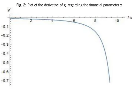
(3.24) 𝑟 = 𝛿𝛼 (1 + 𝛽)(1 − 𝛼)𝐿𝑌(1 − 𝛼𝑙(𝑤̅) 1 − 𝛼) where (3.25) 𝑙(𝑤̅) ≡(1 − 𝜌(𝑤̅)(Γ(𝑤̅) − ℎΦ(𝑤̅))) 𝜌(𝑤̅)

39 (3.26) { 𝑔_𝑐 = 1 𝜎(𝑟 − 𝜌) 𝑔_𝑌 = 𝛿𝐿̅ −𝑟(1 + 𝛽)(1 − 𝛼) 𝛼 (1 −𝛼𝑙(𝑤_{1 − 𝛼}̅)) 𝐾(𝑡)̇ = 𝑌(𝑡) − 𝐶(𝑡) − ∫ (𝑃_𝐴(𝜏) − 𝛽(𝜏)𝑃_𝐴(𝜏))𝑑𝜏 𝑡 0

which, because of the transversality condition (3.3), and because the model is to hold over an infinite horizon, gives us the balanced growth path solution

(3.27)

𝑔 =

𝛿𝐿̅𝛼 (1 −𝛼𝑙(𝑤_{1 − 𝛼}̅)) − 𝜌(1 + 𝛽)(1 − 𝛼) 𝛼 (1 −𝛼𝑙(𝑤_{1 − 𝛼}̅)) + 𝜎(1 + 𝛽)(1 − 𝛼)

which is a generalization of the original framework that encompasses the effects of financial frictions in the economy, through 𝑙(𝑤̅). Further details are available in appendix A. What we’ve done to prove equality between the growth rates was to take the limit of 𝐾(𝑡̇ )

𝐾(𝑡) when 𝑡 → ∞.

Because of the transversality condition, the third term disappears, rendering the capital accumulation equivalent to that of Romer’s original framework. Figure 1 represents a simulation ran for the general equilibrium solution.