Biostatistics: fundamental
concepts and practical applications
Bioestatísticas: conceitos fundamentais e aplicações práticas
Bernardo Lopes
1,Isaac C Ramos ¹, Guilherme Ribeiro², Rosane Correa¹, Bruno Valbon¹; Allan Luz¹; Marcella
Salomão¹, João Marcelo Lyra², Renato Ambrósio Junior
1A
BSTRACTThe biostatistics has gained significant importance in recent years, being one of the mainstays of current scientific research. It has a series of concepts and rules that must be understood to carry out or analyze an article. In this review we will discuss some of main tools utilized in works of interest in ophthalmology, its applications and limitations.
Keywords: Biostatistics/methods; Statistical distributions; Data Interpretation, statistical
R
ESUMOA bioestatística ganha crescente importância e relevância nos últimos anos, sendo um dos principais pilares da investigação científica. Possui uma série de conceitos e regras que devem ser bem compreendidos para se realizar ou analisar um artigo. Nesta revisão são abordadas algumasdas principais ferramentas utilizadas nos trabalhos de interesse da área oftalmológica, suas aplicações e limitações.
Descritores: Bioestatística/métodos; Distribuições estatísticas; Interpretação estatística de dados
·
1Rio de Janeiro Corneal Tomography and Biomechanics Study Group, Rio de Janeiro, RJ, Brasil. 2Brazilian Study Group of Artificial Intelligence and Corneal Analysis (BrAIn), Brazil.
The authors declare no conflicts of interest
I
NTRODUCTIONT
he advent of Evidence-Based Medicine has brought new standards and requirements, producing significant change in medical practice. Knowledge is no longer obtained solely through clinical experience, which is important but limited; instead, it is now acquired through the scientific method, which relies on statistics as one of its essential elements(1). Thus,understanding biostatistics is essential to adequately conduct, assess, and interpret scientific work. However, physicians often have difficulties and prejudices related to this area. In this review, we will discuss the practical aspects of some of the key tests of interest to ophthalmology studies.
Hypothesis testing
When conducting a statistical test, the first to do is to develop hypotheses. For example, to assess whether central corneal thickness (CCT), thickness at the thinnest point (TP), and central keratometry values (K1 and K2) can be used to differentiate normal eyes from eyes with keratoconus, two hypotheses should be formulated. The hypothesis that there is no difference in the values of these variables between the two groups is called the null hypothesis (H0), while the alternative hypothesis (H1) assumes that there is a difference between the normal group and the keratoconus group.
Sampling
To start the proposed test the study samples need to be determined. For the results of a study to be valid it is essential that each sample represents the various characteristics of the population as reliably as possible. The most relevant characteristics of a sample include how it was obtained, its size, distribution of variables, and pairing. With this, the potential sources of bias can be identified and the best methods and statistical tests to prevent bias can be selected.
Sample distribution
The sample distribution should be tested to determine whether it is parametric or not. Statistical tests are highly dependent on the distribution of values obtained from the sample. The normal or Gaussian (parametric) distribution is one of the most studied types of distribution in biostatistics. It is defined by two parameters: mean (ì) and variance (ó²). Among its features are the typical bell-shaped symmetrical distribution around the centre and the presence of two inflection points (right and left) whose distance from the centre corresponds to the standard deviation or sigma (ó). Using these data the probabilities related to a continuous variable can be calculated(2).
When the sample is relatively large, the central limit theorem can be applied to infer the normality of the distribution. This theorem states that as the size of a sample increases, the sample distribution of its mean increasingly approaches the nor-mal distribution(3).
However, tests can be used to assess the normality of a distribution. They include the Kolmogorov-Smirnov test, the Lillefors test, and the Shapiro-Wilk test. The latter was initially described for small samples(4). In these tests the aim is to find the
null hypothesis, in which there is no difference between the sample distribution and the normal distribution. In general these tests are quite rigorous and easily reject the hypothesis of normality. Other tools include descriptive methods such as histogram analysis (Figure 1), coefficients of skewness, and kurtosis. When normality can not be inferred, non-parametric tests or data
transformation can be used. The most commonly-used transformation is logarithmic transformation, which is primarily indicated for asymmetrical data. Other transformations such square root or inverse transformation can also be used in certain cases(5).
Dependent and independent samples
In selecting the type of test to use, another feature of the sample should be considered: whether it is paired (dependent) or unpaired (independent). A study with paired samples occurs when each observation in the first group is paired with the same observation in the second group. In ophthalmology, this is most often used where the same sample is observed at two or more different time points, such as pre- and postoperatively. In this case, the two groups are composed of the same individuals.
In unpaired cases each group is composed of distinct individuals, for example in order to compare subjects with a certain disease with healthy subjects.
It is important to highlight this feature of the sample, because two observations in the same individual are more likely to be similar than two observations in two different individuals; therefore, they are more likely to be statistically dependent. This should be considered by the test in order to find the statistical validity of differences between samples.
Another implication of pairing is the fact that the eyes are paired organs. There is a symmetry between the right and left eye of the same individual. If both eyes of a patient are used, dependent and independent data could get mixed, thus producing a methodological error(6). Thus, using only one randomly-chosen
eye of each patient is a good way to conduct studies(7).
Types of tests
Statistical tests should conform to the sample features cited above: distribution and pairing. But in order to select the best test, the number of groups or observations should also be considered. The main tests for each situation are summarised in Flowchart 1.
Example of a study
In the following example we will consider the comparison of two groups. The samples consist of 114 randomly-selected healthy eyes (one eye per subject) and 44 eyes with keratoconus(8). The next step is to determine the study variables.
Since the aim is to assess a variable’s ability to be used as a
Figure 1. Histograms. A: Histogram for K2 showing a normal distribution in patients with healthy corneas. B: Histogram for corneal astigmatism showing a non-normal distribution in patients with healthy corneas.
A
B
Frequency Frequency
Astigmatism
Mean = 45,33 Standard Deviation = 1,473 N = 682
Mean = 0,98 Standard Deviation = 0,757 N = 682
K2
diagnostic test, one should test whether the differences between groups are significant. Knowing that the samples are unpaired, the test should be selected based on whether the distribution is normal (parametric) or not. This test will determine whether the difference could be due to chance. A test such as the Kolmogorov-Smirnov test should be used to verify whether the variables in each group are normally distributed (p>0.05), i.e. whether there is no statistically-significant difference between the data distribution in the sample and the normal distribution. Histograms can also be used to visualise the bell-shaped or Gaussian distribution.
Student’s t test can be used if both samples are parametric. According to the central limit theorem, since this is a large sample with more than 30 individuals, using a parametric test can be considered “correct” a priori. However, if the sample was small and the distribution was not normal, data transformation or a parametric test could be used, as mentioned above. A non-parametric test such as the Mann-Whitney test (Mann-Whitney U test or Wilcoxon rank-sum test) would be a good alternative.
Using the parametric test for the variables K1, K2, CCT, and TP, a p-value (the probability of error in concluding that there is a statistically-significant difference) lower than 0.001 was found (Table 1), confirming that there is a statistically-significant difference between normal and keratoconus eyes for each of these variables. When the same test was used for the axis of astigmatism a p-value of 0.12 was found, i.e., there is a 12% probability of error in concluding that there is significant difference between the two samples. In general, a result is considered statistically significant when there is a 5% chance that the difference found in the sample does not represent a real
difference between the populations, that is, that the result was due to chance alone. Thus, due to this high margin of error, it can be considered that there is no statistically-significant difference between the two populations for this variable (Table 1).
The box-plot and dot-plot charts shown in Figure 2 illustrate the distribution of CCT values in the normal and keratoconus groups. The charts show that although there were significant differences between groups, there is considerable overlap in values , making it impossible to separate them completely. Thus, the variable has limitations in differentiating normal and keratoconus eyes, as this overlap produces a greater chance of error.
Classification errors and cut-off point
Two types of error can occur while trying to classify or differentiate normal and keratoconus eyes using variables such as CCT values. Type I error, or á, refers to a positive result in the group of eyes classified as normal, i.e. a false-positive result. Type II error, or â, refers to a negative result in the group of eyes classified as ill, i.e. a false-negative result (Table 2).
However, whether a diagnostic test (or classifier) is “positive” depends essentially on a set cut-off point. Since the variable is a continuous quantitative or ordinal variable, each value can be tested as a cut-off point to determine the presence or absence of disease. For example, for a CCT cut-off point of 540 ìm (under 540 ìm = keratoconus), 37 (32.4%) of the 114 eyes with normal corneas would present a type I or á error, while only one eye with keratoconus would present a type II or â error. The hypothetical sensitivity and specificity of the test can thus be calculated for each tested cut-off point (Table 3).
Flowchart 1
Normal Keratoconus
Mean ± Standard Deviation Range Mean ± Standard Deviation Range p-value*
K1 42.68 ± 1.47 39.5 - 46.7 49.35 ± 7.64 38.6 - 71.6 < 0.001
K2 43.66 ± 1.58 39.8 - 48.2 51.58 ± 9.1 42.6 - 77.5 <0.001
CCT 550 ± 35 444 - 632 460 ± 57 283 - 548 <0.001
TP 544 ± 35 443 - 629 443 ± 60 254 - 542 <0.001
Astig Axis 97 ± 71 1 - 180 76 ± 64 0 - 179 0.12
* Student’s t test
Table 1
Sensitivity and specificity
Sensitivity is a test’s chance of showing a positive result in an individual affected by a disease. It is calculated using only ill individuals as the ratio between the number of ill subjects that had a positive result (true positives, or TP) and the total number of ill subjects, which also includes false negatives (FN).
Specificity is a test’s chance of showing a negative result in a healthy individual. It is calculated using only healthy individuals as the ratio between the number of healthy subjects that had a negative result (true negatives, or TN) and the total number of healthy subjects, which also includes the false positives (FP).
The concepts of sensitivity and specificity will now be used to quantitatively describe the performance of a diagnostic test by constructing its ROC curve.
ROC1 curve and accuracy of a test
The ROC curve is constructed on a Cartesian plane, with sensitivity in the Y axis and 1 minus specificity (1-S) in the X axis, both in decimal values. Sensitivity and specificity are calculated for each cut-off value and inserted as a point on the plane. The ROC curve is formed by linking these points.
Receiver Operating Characteristic
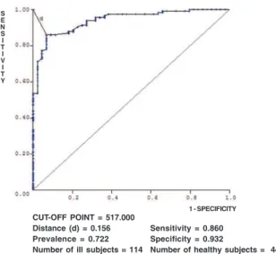
In the case of CCT, the best cut-off value was 517ìm, with a sensitivity of 86% and a specificity of 93.2%. The respective ROC curve can be seen in Figure 3.
The area under the curve (AUC) represents the accuracy or global performance of a test because it considers all the sensitivity and specificity values for each value of the test variable. The greater the test’s power to discriminate between ill and healthy subjects, the more the curve approaches the upper left corner at the point that represents the sensitivity and 1 minus specificity of the best cut-off value. The better the test, the more the area under the ROC curve approaches 1. A test with a weak diagnostic power will show a more flat curve. A test that simply represented chance (like flipping a coin to obtain random binary results) would roughly have a 50% chance of a positive result and a 50% chance of a negative result, regardless of the group, and its area under the curve would be very close to 0.50 (Figure 4).
Comparing areas under ROC curves
After establishing that there is a statistically-significant difference between the variables in healthy and ill patients, it is necessary to determine whether the test has good diagnostic accuracy. As mentioned above, this can be done by building an ROC curve and finding the best cut-off value.
If there are two different diagnostic methods, they can be compared using the area under the ROC curve. To know whether the difference between the two is statistically significant a test is needed to compare them, such as the DeLong test(9). In the Figure 2. Box-plot and dot-plot charts for CCT values
Cut-off point Sensitivity (%) Specificity (%)
< 283 0 100
<= 435 20.45 100
<= 444 20.45 99.12
<= 456 34.09 99.12
<= 459 34.09 98.25
<= 460 36.36 98.25
<= 462 36.36 97.37
<= 477 61.36 97.37
<= 479 63.64 96.49
<= 483 63.64 95.61
<= 493 68.18 95.61
<= 496 68.18 93.86
<= 498 72.73 93.86
<= 501 72.73 91.23
<= 502 75 91.23
<= 504 77.27 90.35
<= 505 79.55 88.6
<= 506 79.55 87.72
<= 507 81.82 87.72
<= 508 81.82 86.84
<= 509 88.64 85.96
<= 516* 93.18 85.96
<= 523 93.18 78.07
<= 524 95.45 77.19
<= 529 95.45 72.81
<= 532 97.73 71.05
<= 547 97.73 53.51
<= 548 100 53.51
<= 632 100 0
Table 3
Sensitivity and specificity for each cut-off point
Test III Group Normal Group
(no disease)
Positive for Correct decision, Type II or β error,
Disease True Positive (TP) False Negative (FN)
Negative for Type I or α Correct decision,
Disease False Positive (FP) True Negative (TN)
Table 2
Results of a diagnostic test
Sensitivity =
TP
(TP+FN)
Specificity =
TN
(TN+FP)
Keratoconus
Normal Normal Keratoconus
Figure 3. ROC curve and cut-off point for CCT in normal versus keratoconus eyes
AUC
K1 0.865
K2 0.859
CCT 0.939
TP 0.957
Table 4
Area under the ROC curve
Table 5
Pairwise comparison of AUCs using the DeLong test (p-values)
previous example with the ROC curves for K1, K2, CCT, and TP variables, it was found that the measures of thickness performed better than the measures of curvature. Among the former, the AUC of TP (0.957) is greater than CCT (0.939). Comparison using the DeLong test shows p=0.003, therefore the higher accuracy of CCT is statistically significant. These results are summarized in Figure 5 and Tables 4 and 5.
Statistical significance versus clinical significance
To verify whether a difference found in a diagnostic test is statistically significant one must calculate the p-value, termed the descriptive level, which is directly related to the test’s power. It can be defined as the “minimum probability of error in concluding that there is statistical significance”(10).
A result is considered to be statistically significant when its p-value is lower than a set value deemed “acceptable” for type I error, which is generally 0.05 (a 5% chance of error, i.e., of concluding that the difference found is significant when it actually reflects chance alone).
Statistical significance, however, is not necessarily the same as clinical significance. The p-value is influenced by sample size. Large samples tend to have lower p-values, and their results tend to have less practical significance. Conversely, small samples tend to have higher p-values.
In this case, although there is clinical relevance, results can be misinterpreted due to the inadequate sample size(11). Therefore
it is not the p-value but AUC that determines the accuracy of a test, as stated above.
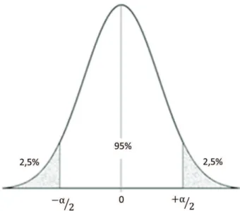
Confidence interval
The concept of confidence interval is related to the variability in accuracy estimates. Its calculation is directly related to type I error or α, as shown in Figure 6. The lower the α, the wider the confidence interval, i.e., the more reliable the estimator. In the example in Figure 6, a 5% á was chosen in a two-tailed
Figure 4. Areas under ROC curves
Figure 5. Comparing ROC curves
S E N S I T I V I T Y
CUT-OFF POINT = 517.000 Distance (d) = 0.156 Prevalence = 0.722 Number of ill subjects = 114
Sensitivity = 0.860 Specificity = 0.932
Number of healthy subjects = 44 1 - SPECIFICITY
TP Astig Axis
K1 K2 CCT TP
K1 K2 CCT TP
K1
K2
CCT
test, therefore there is a 95% probability that the value will be in the range between -α/2 and +α/2. Both the confidence interval and the standard error are calculated based on the sample characteristics and results, being used to interpret the clinical relevance of a diagnostic variable(12).
Improving diagnostic tools
While CCT (K1 and K2) values can not be used alone to differentiate normal and keratoconus eyes, other variables derived from corneal tomography can be considered in isolation or combined(13). Topometric curvature mapping provides data on
the steepest point of the anterior surface. This index is more accurate (higher AUC) than central curvature indices. With tomographic thickness mapping the TP value can be obtained; as seen above, this is a better measure to detect keratoconus than CCT.
Combining variables
To improve diagnostic accuracy even more, different variables can be combined, which can be done through a funda-mental mathematical operation. This is the case of Ambrosio’s Relational Thickness (ART), which is the ratio of corneal thickness at the thinnest point to pachymetric progression. This index has shown a high diagnostic power in detecting keratoconus(8).
Other more sophisticated ways to combine variables are linear discriminant analysis and logistic regression analysis, which can be used to differentiate individuals in groups based on a set of weighted variables. This type of combination is of great value in diagnostic testing, as the method can more accurately differentiate normal and ill patients based on the various data points obtained from tests.
Using the samples above, logistic regression can be performed on data from topographic (Kmax) and tomographic (TP) mapping. The following formula is thus obtained:
This formula is then used to calculate the values for each individual in the sample, obtaining a new variable. By constructing the box-plot and dot-plot charts and the ROC curve a perfect separation between groups is found, as shown in Figure 7. However, formulas obtained through these methods should be validated in other samples to have their applicability demonstrated in diverse populations.
Other more sophisticated methods have been implemented in the study of eye diseases, such as complex artificial intelligence algorithms. It has been shown that such methods significantly increase the effectiveness of disease detection(14,15).
C
ONCLUSIONThis review aimed to present the main concepts of biostatistics and certain tests used to analyse the results of a scientific study and their applicability. This is broad topic and this text does not intend to exhaust it, but only to present a study guide, as the issue is very important in medical practice.
In fact, given the large volume of information produced each day, it is necessary to draw the attention of ophthalmologists to biostatistics, because critical analysis of the statistics with which healthcare professionals deal is critical to improve their clinical practice.
R
EFERENCES1. El Dib RP. [How to practice evidence-based medicine]. J Vasc Bras. 2007;6(1):1-4. Editorial. Portuguese.
2. Abrão FP, Araújo WA, Vieira GM. [Tonometer calibration in Brasília, Brazil]. Arq Bras Oftalmol. 2009;72(3):346-50. Portuguese.
3. Altman DG, Bland JM. Statistics notes: the normal distribution. BMJ. 1995;310(6975):298.
Figure 7. Dot-plot and box-plot charts of logistic regression (LR) created from Kmax and CT, and an ROC curve nearest to the upper left corner (normal: n=114, keratoconus: n=44).
Figure 6. Confidence interval in a two-tailed test, α=5%
- 960,27 + 44,29 * Kmax - 2,27 * TP
LR LR
Normal Keratoconus
4. Flynn MR. Analysis of censored exposure data by constrained maxi-mization of the Shapiro-Wilk W statistic. Ann Occup Hyg. 2010;54(3):263-71.
5. Bland JM, Altman DG. Transformations, means, and confidence inter-vals. BMJ. 1996;312(7038):1079.
6. Holopigian K, Bach M. A primer on common statistical errors in clini-cal ophthalmology. Doc Ophthalmol. 2010;121(3):215-22.cReview. 7. Altman DG, Bland JM. Statistics notes. Treatment allocation in
con-trolled trials: why randomise? BMJ. 1999;318(7192):1209. Review. 8. Ambrósio R Jr, Caiado AL, Guerra FP, Louzada R, Roy AS, Luz A, et
al. Novel pachymetric parameters based on corneal tomography for diagnosing keratoconus. J Refract Surg. 2011;27(10):753-8. 9. DeLong ER, DeLong DM, Clarke-Pearson DL. Comparing the areas
under two or more correlated receiver operating characteristic curves: a nonparametric approach. Biometrics. 1988;44(3):837-45.
10. Paes ÂT. Itens essenciais em bioestatística. Arq Bras Cardiol. 1998;71(4):575-80.
11. Altman DG, Bland JM. Absence of evidence is not evidence of ab-sence. BMJ. 1995;311(7003):485.
12. Azeredo AP. Prestígio clínico da estatística. Rev Bras Oftalmol. 2007;66(6):367-8. Editorial.
13. Ambrósio R Jr, Belin MW. Imaging of the cornea: topography vs to-mography. J Refract Surg. 2010;26(11):847-9.
14. Maeda N, Klyce SD, Smolek MK. Neural network classification of corneal topography. Preliminary demonstration. Invest Ophthalmol Vis Sci. 1995;36(7):1327-35. Erratum in: Invest Ophthalmol Vis Sci 1995;36(10):1947-8.
15. Lyra JM, Machado AP, Ventura BV, Ribeiro G, Araújo LP, Ramos I, et al. Applications of artificial intelligence techniques for improving to-mographic screening for ectasia. In: Belin MW, Khachikian SS, Ambrósio Jr R. Elevation based corneal tomography. City of Knowl-edge: Jaypee Highlights Medical Publishers; 2012. p.123-36.
Corresponding author: