Laboratory Evaluation of the Shinyei
PPD42NS Low-Cost Particulate Matter Sensor
Elena Austin1*, Igor Novosselov2, Edmund Seto1, Michael G. Yost1
1Department of Environmental and Occupational Health Sciences, University of Washington, Seattle, WA, United States of America,2Department of Mechanical Engineering, University of Washington, Seattle, WA, United States of America
*elaustin@uw.edu
Abstract
Objective
Finely resolved PM2.5 exposure measurements at the level of individual participants or over a targeted geographic area can be challenging due to the cost, size and weight of the monitoring equipment. We propose re-purposing the low-cost, portable and lightweight Shi-nyei PPD42NS particle counter as a particle counting device. Previous field deployment of this sensor suggests that it captures trends in ambient PM2.5 concentrations, but important characteristics of the sensor response have yet to be determined. Laboratory testing was undertaken in order to characterize performance.
Methods
The Shinyei sensors, in-line with a TSI Aerosol Particle Sizer (APS) model 3321, tracked particle decay within an aerosol exposure chamber. Test atmospheres were composed of monodisperse polystyrene spheres with diameters of 0.75, 1, 2 3 and 6 um as well as a polydisperse atmosphere of ASHRAE test dust #1.
Results
Two-minute block averages of the sensor response provide a measurement with low ran-dom error, within sensor, for particles in the 0.75–6μm range with a limit of detection of 1μg/
m3. The response slope of the sensors is idiomatic, and each sensor requires a unique response curve. A linear model captures the sensor response for concentrations below 50μg/m3 and for concentrations above 50μg/m3a non-linear function captures the
response and saturates at 800μg/m3. The Limit of Detection (LOD) is 1μg/m3. The
response time is on the order of minutes, making it appropriate for tracking short-term changes in concentration.
Conclusions
When paired with prior evaluation, these sensors are appropriate for use as ambient particle counters for low and medium concentrations of respirable particles (<100 ug/m3). Multiple
sensors deployed over a spatial grid would provide valuable spatio-temporal variability in OPEN ACCESS
Citation:Austin E, Novosselov I, Seto E, Yost MG (2015) Laboratory Evaluation of the Shinyei PPD42NS Low-Cost Particulate Matter Sensor. PLoS ONE 10(9): e0137789. doi:10.1371/journal. pone.0137789
Editor:Jeffrey Shaman, Columbia University, UNITED STATES
Received:May 8, 2015
Accepted:August 21, 2015
Published:September 14, 2015
Copyright:© 2015 Austin et al. This is an open access article distributed under the terms of the Creative Commons Attribution License, which permits unrestricted use, distribution, and reproduction in any medium, provided the original author and source are credited.
Data Availability Statement:All relevant data are within the paper and its Supporting Information files.
PM2.5 and could be used to validate exposure models. When paired with GPS tracking, these devices have the potential to provide time and space resolved exposure measure-ments for a large number of participants, thus increasing the power of a study.
Introduction
Exposure to fine particulate matter (PM2.5) air pollution is associated with a variety of adverse health outcomes, including all-cause mortality, cardiovascular disease, cardiopulmonary dis-ease, and lung cancer [1–9]. The health burden attributable to PM2.5 exposures is large: the most recent global assessment estimates 3.3 million deaths (7.1% of the world’s deaths in 2004) were attributable to PM2.5 exposure, including 2.5 million cardiopulmonary disease and 1.3 million ischemic heart disease deaths [10]. These estimates are higher than previous World Health Organization estimates [11], reflecting improvements in exposure assessment [12]. Even in regions of the developed world, where strong health-protective standards exist, efforts to reduce the impacts of air pollution continue. For example, in the United States, 123 counties do not meet the 24-hour PM2.5 standard [13], and short-term increases in PM2.5 levels are estimated to cause tens of thousands of excess deaths per year [7,14–16].
Efforts to understand aerosol dynamics, reduce PM2.5 concentrations in communities, inform environmental justice studies, reduce exposure assessment errors for epidemiologic studies, and facilitate new models of community-led or community-engaged research may ben-efit from improved understanding of the spatiotemporal distribution of PM with respect to mobile and stationary sources of particulate emissions. Due to the limitations in the coverage and density of U.S. EPA monitoring sites, various modeling approaches have been used to spa-tially resolve air pollution patterns in urban areas and map pollutants on finer scales [17]. An alternative to modeling that provides ongoing empirical data on air pollution concentrations at the neighborhood level, involves augmenting the existing network of EPA sites, with additional monitoring locations [18]. The cost of Federal Reference Method (FRM) continuous monitor-ing PM2.5 instruments, has made it infeasible to establish large dense networks of real-time FRM aerosol monitors. But, short-term monitoring studies of certain urban environments, notably immediate areas downwind of major roadways, have measured elevated concentrations of ultrafine PM, black carbon (BC), elemental carbon (EC) and metals [19],which have led to efforts to protect public health [20].
The recent availability of new low-cost optical aerosol sensors based on the principle of par-ticle light scattering, has motivated new research to evaluate their performance characteristics. We are interested in understanding the environmental health applications in which such sen-sors may be useful, as well as understanding the limitations of these sensen-sors in terms of sensi-tivity, upper and lower limits of detection, sensor to sensor variability, and the dynamics of their response to changing concentrations. This current study builds upon prior work in which we conducted field calibrations of a low-cost sensor, the Shinyei PPD42NS [21]. In that study, the sensor was co-located with a various commercially available particle counters as well as a Federal Equivalent Method (FEM) beta attenuation monitor. Short-term measurements indi-cated strong correlation between the Shinyei and particle counters costing orders of magnitude more. Long-term measurements (approximately 4 months) indicated lower, but still moder-ately good correlation with the FEM beta attenuation monitor. In addition, this sensor was deployed in a high concentration urban setting alongside reference optical and gravimetric methods and shown to have good correlation [22]. While these studies suggest that the sensor
could be used to augment existing regulatory monitoring networks, they also raise numerous questions as to the limits of the sensor’s performance that are best answered in more controlled laboratory environments. This study presents our findings from laboratory work, evaluating the Shinyei PPD42NS for a variety of known particle compositions and concentrations.
Methods and Materials
The Shinyei PPD42NS
The Shinyei PPD42NS is an inexpensive particle counter that costs approximately $10 in small quantities, and can be obtained easily from various electronics retailers (Fig 1). It consists of a light chamber that routes air past a light emitting diode and photo-diode detector that mea-sures the near-forward scattering properties of particles in the air stream. A resistive heater located at the bottom inlet of the light chamber helps move air convectively from the bottom inlet to the top outlet of the chamber. Additional electronics control the underlying detection and signal processing, which results in a digital pulse width modulated output. The raw sensor signal consists of low pulse occupancy (a duration of time that digital signal is held low), which is proportional to particle count concentration. For our laboratory experiments the PPD42NS was connected to a small custom microprocessor circuit developed by our group that reads and stores the low pulse occupancy signals at 1-second intervals.
Laboratory Chamber and Reference Instrument
The comparison instrument for this test was a TSI Aerodynamic Particle Sizer (APS) Spec-trometer 3321. This instrument provides real-time size-resolved counts for particles ranging in size from 0.5–20 microns. Mass is not directly measured by this instrument. However, for
Fig 1. Shinyei PPD42NS.On the left is an exterior image of the sensor. On the right a view of the inside showing the positioning of the various sensor components. (A) Exterior view of sensor. (B) Interior view of sensor. This image was initially published on http://www.takingspace.org/make-your-own-aircasting-particle-monitor
polystyrene particles of known diameter, this instrument provides highly accurate count and mass data [23,24]. Particle count information is converted to mass by inputting the known density of polystyrene beads usingEq 1:
dM¼dNp
6 D
3
pr ð1Þ
Where the density (ρ) is that of the material being aerosolized, the change in number
con-centration (dN) and the diameter of the particle (Dp) are directly measured by the APS as aero-dynamic diameter.
The inherent assumption in this calculation is that the particles are spherical which is true in the case of the polystyrene test aerosol. The number concentration of the test aerosol was maintained below 1500 #/cc to minimize the coincidence errors in the APS counts. Size distri-butions of the test aerosols are provided in the supporting information to demonstrate the monodisperse properties of the aerosol generated. We tested four different PPD42NS sensors over the course of this lab study. The sensors were labeled 1 through 4 and were tested in pairs.
Two sensors were mounted along the interior wall of an airtight box that measured 6 x 21 x 8 cm. This box was placed downstream of the mixing chamber described in the following para-graph. The interior volume within the box was reduced to approximately 500 cm3by placing a fixed baffle along the inner length of the box (Fig 2). Air was actively aspirated at 5 lpm through
Fig 2. Schematic of Experimental Set-Up.The blue circles indicate the location of the mixing fans inside the chamber.
the sensor enclosure using the internal pump of the APS. The sensors were placed in the air-tight enclosure arranged in series upstream of the APS inlet. Static-dissipative silica rubber tub-ing (McMaster-Carr) was used to minimize particle deposition on the inner walls of the sampling train. The sensors were provided 5V of power, as per their operating instructions, output was captured by an Arduino microcontroller and output to a laptop using a serial con-nection. The raw sensor output is on the 1 second reporting interval. Raw sensor output corre-sponds to the photodiode pulse width in a 1 s period. This is called the Lo Pulse Occupancy by the manufacturer and is purported to be proportional to PM2.5mass concentration.
Two different chambers were used as part of these experiments. The first, was 0.3 m3in vol-ume and maintained a slight negative pressure through an exhaust flow. This flow was set at 5 lpm (with a tolerance of 20%). Mixing fans were located in the corners of the chamber to ensure the air was well-mixed. The second chamber was a bench-top model with an internal volume of 0.45 m3. Walls were acrylic and all inputs were sealed. Negative pressure was main-tained through outflow to the APS and sensors (5 lpm). The same aerosol generating mecha-nism was used for both these chambers. The size distribution of the particles between the two chamber set-ups was very similar for the 1μm particles (S3 FigandS4 Fig). In addition, the
half-life of the particles in each experiment was similar (25 ± 3 minutes residence time).
Experimental approach
Test aerosols considered during this series of experiments were monodisperse 0.75, 1.0, 3.0 and 6.0μm polystyrene microspheres in solution (Polysciences, Inc. Warrington, PA); polydisperse
ASHRAE test dust #1. ASHRAE 52.1/52.2 standard test dust composed of 72% ISO 12103–1, A2 Fine Test Dust, 23% powdered carbon and 5% milled cotton linters (purchased from Air Filter Testing Laboratories, Inc. 4632 Old LaGrange Road Buckner, KY). Size distributions of this test atmosphere is provided as supporting information (S1 Fig).
Aerosol, both liquid and dry dust, was generated using a Lovelace nebulizer and introduced into the chamber using 1.5 meter, 2”diameter stainless steel tubing and mixed with a 5 lpm dry air flow to allow for drying prior to introduction. The stainless steel tubing was heated using a heated tape set to 200 C. Aerosol was generated until the concentration inside the chamber was above 1000 #/cc. The aerosol generation then was halted and the decay of the remaining parti-cles was tracked using both the APS and the sensors in series. A small exhaust flow was main-tained throughout the experiments.
Analyses
All collected data were time-matched to the nearest second prior to analysis. The APS data were aggregated over 5-second intervals, and a spline function was used to interpolate concen-trations between these 5-second time points. The Shinyei sensors collected data over 1-second intervals. After being time-matched, the data were transformed using a 2-minute moving aver-age. Models were fit individually for each sensor because of sensor-specific responses.
The relationship between mass concentration as determined by the APS and the raw sensor readings (low pulse occupancy) from the Shinyei was described using three alternative models: a linear model, a polynomial model and a Generalized Additive Model (GAM) that incorpo-rated semi-parametric spline terms. The number of terms to include in the polynomial model was determined based on the Bayesian information criteria (BIC). The spline model was devel-oped using thegamfunction in R and fitted with a penalized thin-plate spline created with the
sfunction.
in less than a 0.2 reported change in Lo Pulse occupancy time on the Shinyei sensor. An alter-native saturation point of the sensor response was determined using a non-linear, least squares model. The model is a von Bertalanffy growth equation with two parameters, presented as
Eq 2:
Shinyeii¼A ð1 e
KAPSiÞ ð2Þ
Where A is the asymptotic Shinyei value K is the growth rate.
APSiis the APS concentration at time i Shinyeiiis the Shinyei value at time i
This model was fit to the data using non-linear least square estimates (nls) package in R. This model was chosen because it captured the shape of the experimental curves and it directly estimates the asymptotic growth parameter. The parameters were initialized with starting val-ues of A = 100 and k = 0.1 and all model runs converged within 50 iterations. The estimated value of A was used to calculate the maximum detection limit (APS mass values) of the sensors for different experimental conditions.
The lower limit of detection (LOD) was calculated as 3 times the standard deviation of the sensors’response for readings on the APS that were less than 1μg/m3. To facilitate
interpret-ability, this LOD was converted toμg/m3using the response plot based on exposure to 1μm
and 3μm diameter polystyrene.
Bland-Altman plots were used to judge the correlation between the Shinyei PM2.5reading, after applying our response curve to 1 um polystyrene beads over a range of concentrations. The model applied was the penalized spline model described above. Data were fit using the pre-dictfunction in R. These plots show the mean of the two measured values on the x-axis and the difference between the measurements on the y-axis. In addition, the Bland-Altman plots were used to contrast the performance of the two different non-linear models applied to the data.
The response times of the sensors were judged based on a step-function experiment. The air drawn through the APS and sensors alternated between room air and air from the chamber containing a 1μm polystyrene test atmosphere.
Analysis was performed in R version 3.0.2.
Results
Fig 3shows the response of the four different sensors to a test atmosphere of 1μm polystyrene
beads. The response of the Shinyei sensors compared to the APS was non-linear over the con-centration range examined. For this section, results are presented as a function of mass concen-tration. This is for interpretability with respect to ambient concentrations. As described above, the conversion from number concentration to mass concentration in the case of a monodis-perse aerosol constitutes of a simple constant adjustment. From 0–50μg/m3the response of
the Shinyei was essentially linear for all test atmospheres. Above 50μg/m3the response was
attenuated. InFig 4, the response between 0–50μg/m3is presented. On this more restricted
range, the response of the Shinyei sensors is well-captured by a linear function.Table 1shows the linear fit of two sensors to different test aerosols from 0–50μg/m3. The output of Sensor 2
was not recorded (serial bus malfunction) for the 0.75μm test atmosphere.
The LOD of the Shinyei sensor was calculated based on 348 observations for which the APS measurement was 1μg/m3or less. As with our measurements, these observations were based
concentrations below 50μg/m3to determine that the LOD was:
LOD¼3SD
iSlopei ð3Þ
Where, SD is the standard deviation of the Shinyei readings when exposed to air with less than 1μg/m3particles
Slopeiis the slopes calculated inTable 1.
The LOD for 1μm polystyrene is 1.0μg/m3and for 3μm it is 1.9μg/m3.
In order to capture the non-linear response of the Shinyei sensor to 1μm particles at higher
concentrations two different models were tested. The first was a polynomial model with five terms. Polynomials with 2 to 6 terms were considered, but the 5 term polynomial model was deemed to have a best fit based using the BIC as a statistical criteria. The second was a semi-parametric penalized thin-plate spline model that captured the non-linear relationship between the Shinyei response and the aerosol mass concentration. The advantage of the polynomial model is that it can easily be parametrized and extrapolated. The advantage of the penalized spline model is that it uses the data variability to produce a non-linear fit that best describes the
Fig 3. Response to a test atmosphere composed of 1μm polystyrene beads.This figure includes raw-data and a penalized spline to describe the response shape.
shape of the response while penalizing for overfitting. The results of the two models were com-pared using a Bland-Altman plot in order to select the model with the best predictive power (Fig 5). For concentrations below 150μg/m3the penalized spline models performed better
than the polynomial model, with the difference between the modeled Shinyei and APS
Fig 4. Response to low concentrations of Polystyrene.
measurements consistently below 10% of the mean of the measurements. Therefore, we con-clude that the penalized spline model performs better than the polynomial model, acknowledg-ing that the response differs by sensor, and hence, the splines will be sensor-specific. Although
Table 1. Linear Model for concentrations below 50 ug/m3.The response of the sensors to test atmospheres is given in terms of a linear slope and error.
Sensor 1 Sensor 2
Slope adj. R2 Slope adj. R2
0.75μm 1.02±0.06 0.66 -
-1.00μm 3.05±0.05 0.99 2.75±0.18 0.98
2.00μm 5.13±0.05 0.99 5.25±0.03 0.99
3.00μm 12.00±0.17 0.99 9.93±0.07 0.99
6.00μm 12.43±0.13 0.86 25.79±0.33 0.80
ASHRAE 5.40±0.03 0.97 8.15±0.04 0.97
doi:10.1371/journal.pone.0137789.t001
Fig 5. Bland Altman Plots (4 sensors pooled together).The red dashed lines represent a 10% error on the mass measurement. The black vertical dashed line represents the LOD.
the spline model produces a semi-parametric response, it can still be used to convert Shinyei observations to equivalent APS measurements using a prediction function implemented in R.
The von Bertalanffy growth equation (Eq 2) allowed for the estimation of the saturation point for the different experimental atmospheres.Table 2presents these results for all polysty-rene experiments. Because the ASHRAE atmosphere was not generated in concentrations high enough to estimate the maximum response, these were not included in this table.
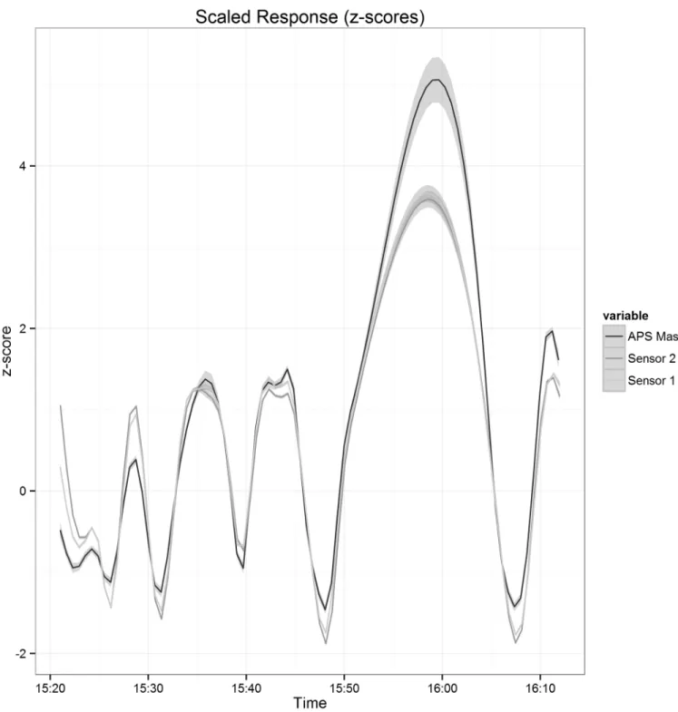
The result of the response time experiment was presented graphically in order to judge the response time of the instruments (Fig 6). The time it took for the instruments to return to a baseline reading after the exposure was switched from polystyrene to filtered air was deter-mined as the response time in this experiment. The mean response time, over 4 repetitions, was 3m:45s (sd 27s) for the APS, 3m:45s (sd 8s) for sensor 1 and 3m:50s (sd 1s) for sensor 2. Thus, the response time of the Shinyei is highly comparable to that of the APS, typically judged to be a fast response instrument.
Discussion
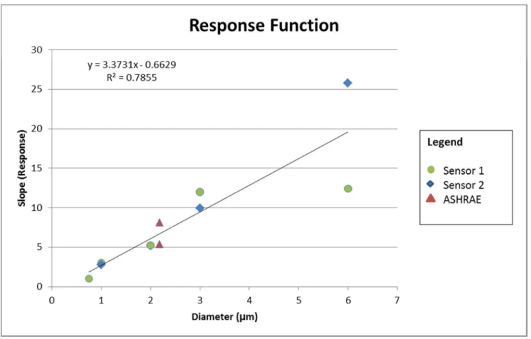
Several questions were explored in this comparison between the Shinyei particle counter and the validated TSI APS instrument that could not be determined in field deployments. The first was the LOD of the Shinyei to a variety of particle sizes, which proves to be low enough to make this an appropriate sensor in most ambient and indoor conditions. The second was the relationship between the sensor response and particle diameter. In fact, as can be expected from an instrument relying on the principle of near-forward scattering, there is a linear rela-tionship between particle diameter and sensor response (Fig 7). For particles under 3 um, the relationship is consistent for the different sets of experimental conditions. For particles in the 6 um diameter range, the response is consistent with the established linear trend, but clearly sub-ject to unacceptable variability for use in field conditions. This suggests that these sensors would benefit from the addition of a size-selective inlet in order to reduce interference from particles with aerodynamic diameters greater than 2.5μm.Fig 7also indicates that the smallest
particle detected with this sensor is 0.5μm. We conclude that this particle sensor is best suited
to detecting particles in the accumulation mode, but is not appropriate for assessing exposures to ultrafine or coarse mode particles.
This comparison also demonstrates that the precision of the Shinyei sensors, when com-pared to the APS is quite high with extremely small standard deviations estimated for the slope and high R2(Table 1). In addition, when the results of all the experiments are pooled, the response of the instruments is highly associated with the diameter of the challenge particle (R2= 0.80). The Bland-Altman plots demonstrated that when the sensors are corrected for their idiomatic response, the results agree with the APS count data within 10% for concentra-tions below 150μg/m3. This suggests that the accuracy of the Shinyei, when the idiomatic
sen-sor response is accounted for, is acceptable for deployment conditions.
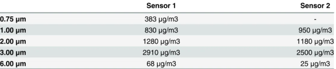
Table 2. Maximum detection limit (determined by modeling sensor response).
Sensor 1 Sensor 2
0.75μm 383μg/m3
-1.00μm 830μg/m3 950μg/m3
2.00μm 1280μg/m3 1180μg/m3
3.00μm 2910μg/m3 2500μg/m3
6.00μm 68μg/m3 25μg/m3
The Shinyei sensors can be reliably used to detect particles ranging in size from 0.5–2.5μm
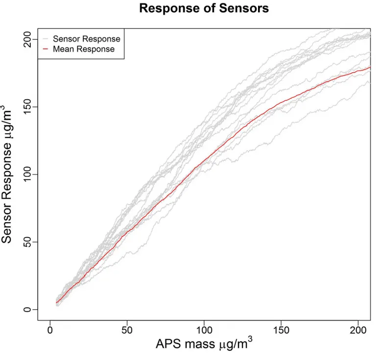
within a set of specified conditions. This corresponds to particles in the respirable range as described by the EPA. The response of these sensors to generated aerosol atmospheres is idio-matic, meaning each sensor follows its own response curve. This was further confirmed by
Fig 6. Response time of the sensors and APS to changes in concentration of a 1μm test atmosphere.
testing of a 20 additional sensors using a 2μm polystyrene test atmosphere (Fig 8) using the
same set-up described above. In addition, the accuracy of the mean response of these 20 sensors in the linear 0–50μg/m3range was judged to be 9% after converting each sensor response to a
mass concentration using a linear regression, as described in the methods section. These results are presented in the supporting information (S7 Fig). Therefore, before being deployed, each sensor requires comparison, either through co-location or laboratory challenges, along the entire range expected to be encountered during sampling. This could be accomplished as we have in this study with a test chamber with monodisperse 1μm polystyrene beads, or
alterna-tively as we have done previously by colocation with reference instruments [21,22]. Secondly, the magnitude of the response of the sensors depends on the diameter of particles being mea-sured. The change in slope between 1 and 3μm polystyrene beads is consistent between
sen-sors; however the response to larger particles is highly variable. This suggests that these sensors would benefit from the addition of a size-selective inlet in order to reduce interference from particles with aerodynamic diameters greater than 2.5μm.
The saturation of the sensors at moderately high concentrations has relevance to their use in certain applications. For ambient monitoring within European and North American urban environments these sensors have adequate limits of detection and maximum limits of detec-tion. However, if these monitors are to be used in environments with PM2.5concentrations
Fig 7. Relationship between sensor response and particle diameter.
that routinely exceed 500μg/m3, they will likely saturate and possibly not capture the true
range of concentrations. Therefore, in these types of monitoring situations other sensors, or possibly dilution with a filtered air stream should be considered.
Because of the low-cost associated with these sensors, and the possibility to calibrate them for field use, they can serve as new tool to reliably obtain continuous exposure estimates over finely detailed spatial areas. The results of this paper suggest that if such sensors are deployed in communities to augment current regulatory monitoring networks, measurements are
Fig 8. Idiomatic response of Shinyei sensors.
expected to be reasonably accurate and precise. However, the conversion from particle count to mass concentrations may be difficult. A possible solution would be to centrally locate a vali-dated method such as an impactor or TEOM in order to calibrate the sensor data. Having a continuous monitoring network with high spatial coverage would have the advantage of allow-ing for more accurate exposure estimates. This type of coverage would also be valuable in cali-brating spatio-temporal PM2.5distribution models. Future work needs to be performed to assess the parameters of such a network given the inherent errors associated with individual sensors as well as inherent errors associated with the deployment of a large number of sensors over a small spatial area.
The small size, low power requirements and the ability for the Shinyei sensors to be inte-grated with other monitoring devices such as GPS or mobile phones, make this sensor a prom-ising tool for personal monitoring studies, in which a study participant could wear such a monitor. The ability to obtain detailed continuous exposure information from a large number of study participants may allow for additional insight into the association between short-term exposures to respirable PM2.5and their acute health effects. Such a monitor would might also provide spatial and time resolved data and allow for the determination of where and when indi-vidual participants receive the bulk of their exposure. Again, the applicability of the Shinyei to personal monitoring studies largely depends on whether the upper limit of detection might be exceeded. The monitor could be saturated in certain occupational and developing world studies.
One important limitation to integrating these sensors into larger studies at this time is that we have not evaluated their long-term performance. Possible problems that may arise are drift in the sensor’s response, as well as the sensors failing during deployment. Sensor drift might occur due to deposits forming on the lens of the optical sensor. While we do not know the length of time the sensors can perform without appreciable drift, it is possible to develop field protocols in which sensors are routinely recalibrated. This is no different from the traditional and more costly instruments that also require routine recalibration.
A possible solution to the recalibration concerns may be ongoing field co-locations of the low cost sensors with reference instruments. Routine checks for deviation over time from initial calibration curves, may indicate that it may be time to recalibrate all the deployed sensors in a network, through some combination of cleaning the lenses, replacing worn sensors (after all, they are inexpensive), and re-estimation of the individual calibration regression models. Such a protocol might accommodate regional variations in drift time. For example, deviations from the original calibration curves might occur quicker in higher concentration applications.
The sensor may have use outside of ambient air monitoring situations including indoor monitoring and in-vehicle monitoring. Recent work by Burnet et al., 2014 has described poten-tial real-world exposures to different types of PM2.5as spanning orders of magnitude in range of concentration. This implies that the maximal response concentration of the sensors must be considered when designing an exposure assessment study.Table 2presents the maximum detection limit of these sensors for different particles sizes, based on modeling the responses obtained in this laboratory study. Based on these results it may not be appropriate to deploy these sensors in locations with high indoor particle concentration. Because the sensitivity of the sensor decreases as the concentrations approaches the maximum detection limit, distin-guishing between levels of exposure at high concentrations may not be possible using this monitor.
5-minute average concentration of PM2.5in the homes of smokers (n = 58) in the UK was 491μg/m3in the maximum 5-minute average concentration in the home of smokers was much
higher than the maximum 5-minute average in the home of non-smokers. The Shinyei sensors might be useful for counting smoking events in the home. Another important source on indoor exposure to PM2.5is biomass burning. In Pakistan Siddiqui et al. [26] reported that mean day-time concentration of PM2.5in homes using wood as fuel was 2.74 mg/m3.The Shinyei sensors could be useful in monitoring biomass cooking and/or heating events but would fail to discrim-inate between exposure levels in different homes using biomass sources.
We conclude that the sensitivity of this sensor is appropriate for most outdoor locations within the US and Europe, but without modification of the sensor, may not be adequate to cap-ture the full range of higher indoor exposures in homes of smokers or homes where biomass is a source of energy for heat or cooking. It is important to remember that the sensor is a particle counter, and in cases of exposure to polydisperse aerosol of unknown composition, conversion to mass may be difficult without the availability of a concurrent gravimetric sample.
Supporting Information
S1 Data. Underlying data used to generate figures and tables in this paper.Includes the time matched response of the APS and Shinyei sensors for a variety of test atmospheres. (XLSX)
S1 Fig. Size Distribution of ASHRAE dust. (DOCX)
S2 Fig. Distribution of the 0.75μm polystyrene test atmosphere. (DOCX)
S3 Fig. Distribution of the 1μm polystyrene test atmosphere (Large Chamber). (DOCX)
S4 Fig. Distribution of the 1μm polystyrene test atmosphere (Small Chamber). (DOCX)
S5 Fig. Distribution of the 3μm polystyrene test atmosphere. (DOCX)
S6 Fig. Distribution of the 6μm polystyrene test atmosphere. (DOCX)
S7 Fig. Percent difference between the mean sensor response and APS values after convert-ing the sensor response to a mass concentration usconvert-ing a linear regression.
(DOCX)
Acknowledgments
The authors would like to thank the Department of Environmental and Occupational Health Sciences at the University of Washington for its support of this project.
Author Contributions
References
1. Dockery DW, Pope CA III, Xu X, Spengler JD, Ware JH, Fay ME, et al. An association between air pol-lution and mortality in six US cities. N Engl J Med 1993; 329(24):1753–1759. PMID:8179653 2. Krewski D, Burnett RT, Goldberg MS, Hoover K, Siemiatycki J, Jerrett M, et al. Reanalysis of the
Har-vard Six Cities Study and the American Cancer Society Study of particulate air pollution and mortality. Cambridge, MA: Health Effects Institute 2000;295.
3. Krewski D, Jerrett M, Burnett RT, Ma R, Hughes E, Shi Y, et al. Extended follow-up and spatial analysis of the American Cancer Society study linking particulate air pollution and mortality.: Health Effects Insti-tute Boston, MA; 2009.
4. Lipfert F, Wyzga R, Baty J, Miller J. Traffic density as a surrogate measure of environmental exposures in studies of air pollution health effects: Long-term mortality in a cohort of US veterans. Atmos Environ 2006; 40(1):154–169.
5. Peng RD, Dominici F, Pastor-Barriuso R, Zeger SL, Samet JM. Seasonal analyses of air pollution and mortality in 100 US cities. Am J Epidemiol 2005 Mar 15; 161(6):585–594. PMID:15746475
6. Pope CA III, Burnett RT, Thun MJ, Calle EE, Krewski D, Ito K, et al. Lung cancer, cardiopulmonary mor-tality, and long-term exposure to fine particulate air pollution. JAMA 2002; 287(9):1132–1141. PMID: 11879110
7. Pope CA 3rd, Dockery DW. Health effects of fine particulate air pollution: lines that connect. J Air Waste Manag Assoc 2006 Jun; 56(6):709–742. PMID:16805397
8. Samet JM, Dominici F, Curriero FC, Coursac I, Zeger SL. Fine particulate air pollution and mortality in 20 U.S. cities, 1987–1994. N Engl J Med 2000 Dec 14; 343(24):1742–1749. PMID:11114312 9. Zeger SL, Dominici F, McDermott A, Samet JM. Mortality in the Medicare population and chronic
expo-sure to fine particulate air pollution in urban centers (2000–2005). Environ Health Perspect 2008; 116 (12):1614–1619. doi:10.1289/ehp.11449PMID:19079710
10. Evans J, van Donkelaar A, Martin RV, Burnett R, Rainham DG, Birkett NJ, et al. Estimates of global mortality attributable to particulate air pollution using satellite imagery. Environ Res 2013; 120:33–42. doi:10.1016/j.envres.2012.08.005PMID:22959329
11. Cohen AJ, Ross Anderson H, Ostro B, Pandey KD, Krzyzanowski M, Künzli N, et al. The global burden of disease due to outdoor air pollution. Journal of Toxicology and Environmental Health, Part A 2005; 68(13–14):1301–1307.
12. van Donkelaar A, Martin RV, Brauer M, Kahn R, Levy R, Verduzco C, et al. Global estimates of ambient fine particulate matter concentrations from satellite-based aerosol optical depth: development and application. Environ Health Perspect 2010 Jun; 118(6):847–855. doi:10.1289/ehp.0901623PMID: 20519161
13. US EPA.Fine Particle (PM2.5) Designations. 2013; Available:http://www.epa.gov/airquality/ particlepollution/designations/index.htm. Accessed 2014 Aug 11.
14. Brook RD, Franklin B, Cascio W, Hong Y, Howard G, Lipsett M, et al. Air pollution and cardiovascular disease: a statement for healthcare professionals from the Expert Panel on Population and Prevention Science of the American Heart Association. Circulation 2004 Jun 1; 109(21):2655–2671. PMID: 15173049
15. Brook RD, Rajagopalan S, Pope CA 3rd, Brook JR, Bhatnagar A, Diez-Roux AV, et al. Particulate mat-ter air pollution and cardiovascular disease: An update to the scientific statement from the American Heart Association. Circulation 2010 Jun 1; 121(21):2331–2378. doi:10.1161/CIR.0b013e3181dbece1 PMID:20458016
16. Simkhovich BZ, Kleinman MT, Kloner RA. Air pollution and cardiovascular injuryepidemiology, toxicol-ogy, and mechanisms. J Am Coll Cardiol 2008; 52(9):719–726. doi:10.1016/j.jacc.2008.05.029PMID: 18718418
17. Jerrett M, Arain A, Kanaroglou P, Beckerman B, Potoglou D, Sahsuvaroglu T, et al. A review and evalu-ation of intraurban air pollution exposure models. Journal of Exposure Science and Environmental Epi-demiology 2004; 15(2):185–204.
18. Clougherty JE, Kheirbek I, Eisl HM, Ross Z, Pezeshki G, Gorczynski JE, et al. Intra-urban spatial vari-ability in wintertime street-level concentrations of multiple combustion-related air pollutants: the New York City Community Air Survey (NYCCAS). J Expo Sci Environ Epidemiol 2013 May-Jun; 23(3):232– 240. doi:10.1038/jes.2012.125PMID:23361442
19. Karner AA, Eisinger DS, Niemeier DA. Near-roadway air quality: synthesizing the findings from real-world data. Environ Sci Technol 2010; 44(14):5334–5344. doi:10.1021/es100008xPMID:20560612 20. California Environmental Protection Agency. Air Quality and Land Use Handbook: A Community Health
21. Holstius D, Pillarisetti A, Smith K, Seto E. Field calibrations of a low-cost aerosol sensor at a regulatory monitoring site in California. Atmospheric Measurement Techniques Discussions 2014; 7(1):605–632. 22. Gao M, Cao J, Seto E. A distributed network of low-cost continuous reading sensors to measure
spatio-temporal variations of PM2. 5 in Xi'an, China. Environmental pollution 2015; 199:56–65. doi:10.1016/j. envpol.2015.01.013PMID:25618367
23. Volckens J, Peters TM. Counting and particle transmission efficiency of the aerodynamic particle sizer. J Aerosol Sci 2005; 36(12):1400–1408.
24. Stein SW, Myrdal PB, Gabrio BJ, Obereit D, Beck TJ. Evaluation of a new Aerodynamic Particle Sizer spectrometer for size distribution measurements of solution metered dose inhalers. Journal of Aerosol Medicine 2003; 16(2):107–119. PMID:12823905
25. Osman LM, Douglas JG, Garden C, Reglitz K, Lyon J, Gordon S, et al. Indoor air quality in homes of patients with chronic obstructive pulmonary disease. American journal of respiratory and critical care medicine 2007; 176(5):465–472. PMID:17507547