The Standard of Living and the Satisfaction of the Ideal Job, the Perceptions of the Well-Being and Happiness in Romania

Annals of “Dunarea de Jos” University of Galati Fascicle I. Economics and Applied Informatics

Years XXII – no_3/2016

ISSN-L 1584-0409 ISSN-Online 2344-441X

www.eia.feaa.ugal.ro

The Standard of Living and the Satisfaction of the Ideal

Job, the Perceptions of the Well-Being and Happiness in

Romania

Gabriela OPAIT

A R T I C L E I N F O A B S T R A C T

Article history: Accepted November Available online December JEL Classification C , C , C

Keywords:

Standard of Living, Satisfaction of the )deal Job, Well-Being, (appiness

This research reflects the architecture of the methodology for to achieve the statistical modeling of the trends concerning the Standard of Living and the Satisfaction of the )deal Job in Romania, between - with the help of the „Least Squares Method”. The Standard of Living reflects the level of comfort and also, the level of wealth for a certain socio-economic class. The Standard of Living reflects our material welfare and this indicator represents a real vector of the progress concerning the human development.

© EA). All rights reserved.

1. Introduction

)n this paper, ) present a personal contribution which reflects a statistical analysis of the trends model regarding the Standard of Living and the Satisfaction of the )deal Job the in Romania, in the period - . The purpose of the research reflects the possibility for to anticipate the values concerning the Standard of Living and the Satisfaction of the )deal Job in future, in Romania. by means of the forecasting methods. The statistical methods used are the „Coefficients of Variation Method”, respectively the „Least Squares Method”applied for to calculate the parameters of the regression equation. The sections presents the methodology for to achieve the trend model concerning the Standard of Living in Romania, in the period - , with the help of the „Least Squares Method”. The section reflects the architecture concerning the modeling of the trend between the values regarding the Satisfaction of the )deal Job, in Romania, between - . The section expresses the forecasting method reflected by the „Least Squares Method” applied for the Standard of Living, respectively the Satisfaction of the )deal Job in Romania. The state of the art in this domain is represented by the research belongs to Carl Friederich Gauss, who created the „Least Squares

Method”[ ].

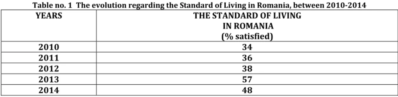
2. The modeling of the trend concerning the Standard of Living in Romania, between 2010-2014. )n the period - , we observe the next evolution regarding the Standard of Living in Romania, according to the table no. :

Table no. 1 The evolution regarding the Standard of Living in Romania, between 2010-2014

YEARS THE STANDARD OF LIVING

IN ROMANIA (% satisfied)

2010 34 2011 36 2012 38 2013 57 2014 48

Source: „Human Development Report” 2015

We want to identify the trend model concerning the Standard of Living in Romania, between the period - , using the table no. .

- if we formulate the null hypothesis

H

0: which mentions the assumption of the existence for the model of

tendency concerning X factor, where X = the Standard of Living in Romania, as being the function

i

t

a

b

t

x

i

=

+

⋅

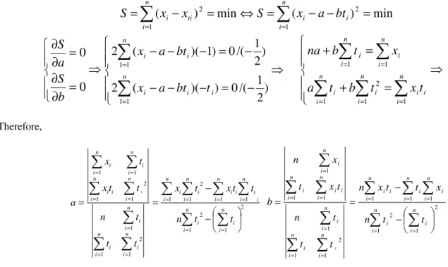
, then the parameters a and b of the adjusted linear function, can to be calculated by means of

the next system [ ]:

∑

∑

= =

=

−

−

=

⇔

=

−

=

n

i

i i

n

i

ti

i

x

S

x

a

bt

x

S

1

2

1

2

min

)

(

min

)

(

⇒

⎪

⎪

⎩

⎪⎪

⎨

⎧

=

∂

∂

=

∂

∂

0

0

b

S

a

S

⇒

⎪

⎪

⎩

⎪⎪

⎨

⎧

−

=

−

−

−

−

=

−

−

−

∑

∑

= =

n

i i i

n

i i

t

bt

a

x

bt

a

x

1 1

1 1

)

2

1

/(

0

)

)(

(

2

)

2

1

/(

0

)

1

)(

(

2

⇒

⎪

⎪

⎩

⎪⎪

⎨

⎧

=

+

=

+

∑

∑

∑

∑

∑

= =

=

= =

n

i i i n

i i n

i i

n

i i n

i i

t

x

t

b

t

a

x

t

b

na

1 1

2

1

1 1

Therefore,

∑

∑

∑

∑

∑

∑

∑

∑

∑

∑

∑

∑

∑

= =

= = = =

= =

= = =

= =

⎟ ⎠ ⎞ ⎜ ⎝ ⎛

− − =

=

n

i

n

i i i

n

i i

n

i i n

i i i n

i i i

n

i i n

i i

n

i i n

i n

i i i

n

i i n

i i

t t

n

t t x t x

t t

t n

t t x

t x

a

i

1

2 1 2

1 1 1 1 2

1 2 1

1 1

2 1

1 1

2

1 1

2

1 1 1

1 2 1

1 1 1

1

⎟ ⎠ ⎞ ⎜ ⎝ ⎛

− − =

=

∑

∑

∑

∑

∑

∑

∑

∑

∑

∑

∑

= =

= = =

= =

= = =

=

n

i i n

i i

n

i i n

i i n

i i i

n

i n

i i

n

i i n

i i i n

i i

n

i i

t t

n

x t t x n

t t

t n

t x t

x n

b

i

Table no. 2 The estimate of the value for the variation coefficient in the case of the adjusted linear function, in the hypothesis of the linear evolution concerning the

Standard of Living in Romania, between 2010-2014

LINEAR TREND

YEARS

THE STANDARD OF LIVING IN ROMANIA (% satisfied)

(xi)

i

t

2

i

t

t

_i

x

_i

i

t

a

bt

x

i

=

+

i

t

i x

x −

2010 34 - - , ,

2011 36 - - , ,

2012 38 , ,

2013 57 , ,

2014 48 , ,

TOTAL 213 ,

)f we calculate the statistical data for to adjust the linear function, we obtain for the parameters a and b the

values:

6 , 42 0

10 5

0 49 10 213

2 =

− ⋅

⋅ − ⋅ = a

4,9 0

10 5

213 0 49 5

2 =

− ⋅

⋅ − ⋅ = b

100

10

,

05

%

213

4

,

21

100

100

:

⋅

=

⋅

=

−

=

⋅

⎥

⎥

⎥

⎥

⎦

⎤

⎢

⎢

⎢

⎢

⎣

⎡

−

=

∑

∑

∑

∑

− = − = − = − = m m i i m m i I t i m m i i m m i I t i I

x

x

x

n

x

n

x

x

v

i i

- in the situation of the alternative hypothesis

H

1: which specifies the assumption of the existence for the

model of tendency regarding X factor, where X= the Standard of Living in Romania,as being the quadratic

function 2

i i

t

a

b

t

ct

x

i

=

+

⋅

+

, the parameters a, b şi c of the adjusted quadratic function, can to be calculated

by means of the system [ ]:

∑

∑

= =

=

−

−

−

=

⇔

=

−

=

n i i i i n i ti

i

x

S

x

a

bt

ct

x

S

1 2 2 1 2

min

)

(

min

)

(

⇒

⎪

⎪

⎪

⎩

⎪

⎪

⎪

⎨

⎧

=

∂

∂

=

∂

∂

=

∂

∂

0

0

0

c

S

b

S

a

S

⇒

⎪

⎪

⎪

⎪

⎩

⎪⎪

⎪

⎪

⎨

⎧

−

=

−

−

−

−

−

=

−

−

−

−

−

=

−

−

−

−

∑

∑

∑

= =

)

2

1

/(

0

)

)(

(

2

)

2

1

/(

0

)

)(

(

2

)

2

1

/(

0

)

1

)(

(

2

2 2 1 1 2 1 1 2 i i i i n i i i i n i i i

t

ct

bt

a

x

t

ct

bt

a

x

ct

bt

a

x

Therefore,

⎪

⎪

⎪

⎩

⎪

⎪

⎪

⎨

⎧

⋅

=

+

+

⋅

⋅

=

+

⋅

+

=

+

+

⋅

∑

∑

∑

∑

∑

∑

∑

∑

∑

∑

∑

= = = = = = = = = = = n i i i n i i n i i n i i n i i i n i i n i i n i i n i i n i i n i i

x

t

t

c

t

b

t

a

x

t

t

c

t

b

t

a

x

t

c

t

b

a

n

1 2 1 4 1 3 1 2 1 1 3 1 2 1 1 1 2 1

∑

∑

∑

∑

∑

∑

= = = = = =

⎟

⎠

⎞

⎜

⎝

⎛

−

⋅

−

=

n i n i i i n i i n i i i n i i n i i i

t

t

n

x

t

t

x

t

a

1 2 1 2 4 1 1 2 1 2 1 4 ;

∑

∑

= =

=

_n i i n i i i

t

t

x

b

1 2 1 ;

∑

∑

∑

∑ ∑

= = = = =

⎟

⎠

⎞

⎜

⎝

⎛

−

⋅

−

⋅

⋅

=

n i n i i i n i n i n i i i i i

t

t

n

x

t

x

t

n

c

1 2 1 2 4

1 1 1

2 2

Table no. 3 The estimates of the value for the variation coefficient in the case of the adjusted quadratic function, in the hypothesis of the parabolic evolution regarding the Standard of Living

in Romania, between 2010-2014

A. PARABOLIC TREND

B. YEARS THE STANDARD OF LIVING IN ROMANIA (% satisfied)

(xi)

3

i

t

t

i4

t

i

x

i

2

2

i i

t

a

bt

ct

x

i

=

+

+

i t i x x −

2010 34 - , ,

2011 36 - , ,

2012 38 , ,

2013 57 , ,

2014 48 , ,

TOTAL 213 ,

₄₃

_,

_31428571

10

34

5

421

10

213

34

2

=

−

⋅

⋅

−

⋅

=

a

; _4,9

10 49

= =

b ;

0

,

357142857

10

34

5

213

10

421

5

2

=

−

−

⋅

⋅

−

⋅

=

c

So, the coefficient of variation for the adjusted quadratic function has the value:

%

38

,

10

100

213

114

,

22

100

100

:

⋅

=

⋅

=

−

=

⋅

⎥

⎥

⎥

⎥

⎦

⎤

⎢

⎢

⎢

⎢

⎣

⎡

−

=

∑

∑

∑

∑

− = − = − = − = m m i i m m i II t i m m i i m m i II t i II

x

x

x

n

x

n

x

x

v

i i

- in the case of the alternative hypothesis

H

₂ : which describes the supposition of the existence for the model

of tendency concerning X factor, where X = the Standard of Living in Romania, as being the exponential

function i

i

t

t

ab

x

=

, then the parameters a and b of the adjusted exponential function, can to be calculated by

means of the next system [ ]:

∑

∑

= =

=

−

−

=

⇔

=

−

=

n i i i n i t

i

x

S

x

a

t

b

x

S

i 1 2 1 2

min

)

lg

lg

(lg

min

)

lg

(lg

⇒

⎪

⎪

⎩

⎪⎪

⎨

⎧

=

∂

∂

=

∂

∂

0

lg

0

lg

b

S

a

S

⇒

⎪

⎪

⎩

⎪⎪

⎨

⎧

−

=

−

−

−

−

=

−

−

−

∑

∑

= = n i i i n i i

t

b

t

a

x

b

t

a

x

1 1 1 1

)

2

1

/(

0

)

)(

lg

lg

(lg

2

)

2

1

/(

0

)

1

)(

lg

lg

(lg

2

⎪

⎪

⎩

⎪⎪

⎨

⎧

⋅

=

⋅

+

=

⋅

+

⋅

∑

∑

∑

∑

∑

= = = = = n i i i n i i n i i n i i n i i

x

t

t

b

t

a

x

t

b

a

n

1 1 2 1 1 1

lg

lg

lg

lg

lg

lg

Thus,

∑

∑

∑

∑

∑

∑

∑

∑

∑

∑

∑

∑

∑

= = = = = = = = = = = = = ⎟ ⎠ ⎞ ⎜ ⎝ ⎛ − − = = n i n i i i n i i n i i n i i i n i i i n i i n i i n i i n i n i i i n i i n i i t t n t x t t x t t t n t x t t x a i 1 2 1 2

1 1 1 1

2 1 2 1 1 1 2 1 1 1 lg lg lg lg lg and

∑

∑

∑

∑

∑

∑

∑

∑

∑

∑

∑

= = = = = = = = = = = ⎟ ⎠ ⎞ ⎜ ⎝ ⎛ − − ⋅ = = n i n i i i n i i n i i n i i i i n i i n i i n i i n i i n i i n i i t t n t x x t n t t t n x t t x n b i 1 2 1 2

1 1 1

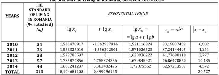
Table no. 4 The estimate of the value for the variation coefficient in the case of the adjusted exponential function, in the hypothesis concerning the exponential evolution regarding

the Standard of Living in Romania, between 2010-2014

EXPONENTIAL TREND

YEARS

THE STANDARD

OF LIVING IN ROMANIA (% satisfied)

(xi)

lg

x

i

t

i

lg

x

i

lg

x

ti

=

b

t

a

_i

lg

lg

+

=

ti

ti

ab

x

=

xi−xt_i

2010 34 , - , , , ,

2011 36 , - , , , ,

2012 38 , , , ,

2013 57 , , , , ,

2014 48 , , , , ,

TOTAL 213 , , ,

Consequently, if we calculate the statistical data for to adjust the exponential function, we obtain for the parameters a and b the values:

1,620936222 0

10 5

0 499096995 ,

0 10 62571684 ,

32

lg ₂ =

− ⋅

⋅ −

⋅ =

a

0,049909699 0

10 5

0 104681108 ,

8 499096995 ,

0 5 lg

2 =

− ⋅

⋅ −

⋅ =

b

Accordingly, the coefficient of variation for the adjusted exponential function has the next value:

%

64

,

9

100

213

527

,

20

100

100

:

exp exp

exp

⋅

=

⋅

=

−

=

⋅

⎥

⎥

⎥

⎥

⎦

⎤

⎢

⎢

⎢

⎢

⎣

⎡

−

=

∑

∑

∑

∑

− = − = −

= −

=

m

m i

i m

m i

t i m

m i

i m

m i

t i

x

x

x

n

x

n

x

x

v

i i

We apply the coefficients of variation method as criterion of selection for the best model of trend. We notice that:

%

38

,

10

%

05

,

10

%

64

,

9

exp

=

<

v

I

=

<

v

II

=

v

So, the path reflected by X factor, which represents the Standard of Living in Romania, between

2010-2014, is an exponential trend of the shape i

i

t

t

ab

x

=

, with other words it confirms the hypothesis

H

2.

We observe that, the cloud of points which reflects the values concerning the Standard of Living in Romania, between - , it carrying around an exponential trend model, according to the type no. .

3. The modeling of the trend regarding the Satisfaction of the Ideal Job in Romania, between 2010-2014

)n the period - , we observe the next evolution concerning the Satisfaction of the )deal Job in Romania, according to the table no. :

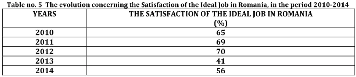
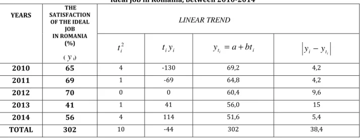
Table no. 5 The evolution concerning the Satisfaction of the Ideal Job in Romania, in the period 2010-2014

YEARS THE SATISFACTION OF THE IDEAL JOB IN ROMANIA

(%)

2010 65 2011 69 2012 70 2013 41 2014 56 The sourse: „(uman Development Report ”

We want to identify the trend model concerning the )deal Job in Romania, between - , using the table no. .

- if we formulate the null hypothesis

H

0: which mentions the assumption of the existence for the model of

tendency concerning

Y

factor, where

Y

= the Satisfaction of the Ideal Job in Romania, as being the function

i

t

a

b

t

y

i

=

+

⋅

, then the parameters a and b of the adjusted linear function, can to be calculated by means of

the next system [ ]:

∑

∑

= =

=

−

−

=

⇔

=

−

=

n

i

i i

n

i

ti

i

y

S

y

a

bt

y

S

1

2

1

2

min

)

(

min

)

(

⇒

⎪

⎪

⎩

⎪⎪

⎨

⎧

=

∂

∂

=

∂

∂

0

0

b

S

a

S

⇒

⎪

⎪

⎩

⎪⎪

⎨

⎧

−

=

−

−

−

−

=

−

−

−

∑

∑

= =

n

i i i

n

i i

t

bt

a

y

bt

a

y

1 1

1 1

)

2

1

/(

0

)

)(

(

2

)

2

1

/(

0

)

1

)(

(

2

⇒

⎪

⎪

⎩

⎪⎪

⎨

⎧

=

+

=

+

∑

∑

∑

∑

∑

= =

=

= =

n

i i i n

i i n

i i

n

i i n

i i

t

y

t

b

t

a

y

t

b

na

1 1

2

1

1 1

Therefore,

∑

∑

∑

∑

∑

∑

∑

∑

∑

∑

∑

∑

∑

= =

= = = =

= =

= = =

= =

⎟ ⎠ ⎞ ⎜ ⎝ ⎛

− − =

=

n

i

n

i i i n

i i

n

i i n

i i i n

i i i

n

i i n

i i

n

i i n

i n

i i i

n

i i n

i i

t t n

t t y t y

t t

t n

t t y

t y

a

i

1

2 1 2

1 1 1 1 2

1 2 1

1 1

2 1

1 1

2 1 1

2

1 1 1

2 1 1 1

1

⎟ ⎠ ⎞ ⎜ ⎝ ⎛

− − =

=

∑

∑

∑

∑

∑

∑

∑

∑

∑

∑

∑

= =

= = =

= = =

=

n

i i n

i i

n

i i n

i i n

i i i

n n

n

i i n

i i i n

i i

n

i i

t t

n

y t t y n

t t

t n

t y t

y n

Table no. 6 The estimate of the value for the variation coefficient in the case of the adjusted linear function, in the hypothesis concerning the linear evolution for the Satisfaction of the

Ideal Job in Romania, between 2010-2014

LINEAR TREND

YEARS

THE SATISFACTION

OF THE IDEAL JOB IN ROMANIA

(%)

(

y

i)

2

i

t

i i

y

t

i

t

a

bt

y

i

=

+

y

i

−

y

t_i

2010 65 - , ,

2011 69 - , ,

2012 70 , ,

2013 41 ,

2014 56 , ,

TOTAL 302 - ,

)f we calculate the statistical data for to adjust the linear function, we obtain for the parameters a and b the

values:

60

,

4

)

0

(

10

5

10

)

44

(

10

302

2

=

−

⋅

⋅

−

−

⋅

=

a

4

,

4

)

0

(

10

5

302

0

)

44

(

5

2

=

−

−

⋅

⋅

−

−

⋅

=

b

(ence, the coefficient of variation for the adjusted linear function is:

%

71

,

12

100

302

4

,

38

100

100

:

⋅

=

⋅

=

−

=

⋅

⎥

⎥

⎥

⎥

⎦

⎤

⎢

⎢

⎢

⎢

⎣

⎡

−

=

∑

∑

∑

∑

− = − = −

= −

=

m

m i

i m

m i

I t i m

m i

i m

m i

I t i

I

y

y

y

n

y

n

y

y

v

i i

- in the situation of the alternative hypothesis

H

1: which specifies the assumption of the existence for the

model of tendency regarding

y

factor, where

y

= the Satisfaction of the Ideal Job in Romania,as being the

quadratic function 2

i

i

c

b

a

i

ξ

ξ

ω

_ξ

=

+

⋅

+

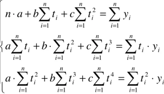
, the parameters a, b şi c of the adjusted quadratic function, can to

be calculated by means of the system [ ]:

∑

∑

= =

=

−

−

−

=

⇔

=

−

=

n

i

i i i

n

i

i

i

y

S

y

a

bt

ct

y

S

1

2 2

1

2

min

)

(

min

)

(

_ξ

⇒

⎪

⎪

⎪

⎩

⎪

⎪

⎪

⎨

⎧

=

∂

∂

=

∂

∂

=

∂

∂

0

0

0

c

S

b

S

a

S

⇒

⎪

⎪

⎪

⎪

⎩

⎪⎪

⎪

⎪

⎨

⎧

−

=

−

−

−

−

−

=

−

−

−

−

−

=

−

−

−

−

∑

∑

∑

= =

)

2

1

/(

0

)

)(

(

2

)

2

1

/(

0

)

)(

(

2

)

2

1

/(

0

)

1

)(

(

2

2 2 1

1

2 1

1

2

i i i i

n

i i i i

n

i i i

t

ct

bt

a

y

t

ct

bt

a

y

ct

bt

a

y

Therefore,

⎪

⎪

⎪

⎩

⎪

⎪

⎪

⎨

⎧

⋅

=

+

+

⋅

⋅

=

+

⋅

+

=

+

+

⋅

∑

∑

∑

∑

∑

∑

∑

∑

∑

∑

∑

= =

= =

= =

= =

= =

=

n

i

i i n

i i n

i i n

i i

n

i i i n

i i n

i i n

i i

n

i i n

i i n

i i

y

t

t

c

t

b

t

a

y

t

t

c

t

b

t

a

y

t

c

t

b

a

n

1 2

1 4

1 3

1 2

1 1

3

1 2

1

1 1

2

1

Table no. 7 The estimates of the value for the variation coefficient in the case of the adjusted quadratic function, in the hypothesis concerning the parabolical evolution for the Satisfaction

of the Ideal Job in Romania, between 2010-2014

PARABOLIC TREND

YEARS

THE SATISFACTI

ON OF THE IDEAL JOB

IN ROMANIA

(%)

(

y

i)

3

i

t

t

i4

t

i

y

i

2

2

i i

t

a

bt

ct

y

i

=

+

+

y

i

−

y

ti

2010 65 - , ,

2011 69 - , ,

2012 70 , ,

2013 41 , ,

2014 56 , ,

TOTAL 302 ,

)f we calculate the statistical data for to adjust the quadratic function, we obtain for the parameters a,b and c

the next values:

61

,

25714286

10

34

5

598

10

302

34

2

=

−

⋅

⋅

−

⋅

=

a

4,4 10 44

− = − = b

0

,

428571428

10

34

5

302

10

598

5

2

=

−

−

⋅

⋅

−

⋅

=

c

So, the coefficient of variation for the adjusted quadratic function has the value:

%

43

,

12

100

302

543

,

37

100

100

:

⋅

=

⋅

=

−

=

⋅

⎥

⎥

⎥

⎥

⎦

⎤

⎢

⎢

⎢

⎢

⎣

⎡

−

=

∑

∑

∑

∑

− = − = −

= −

=

m

m i

i m

m i

II i m

m i

i m

m i

II i

II

i i

n

n

v

ω

ω

ω

ω

ω

ω

_{ξ ξ}

- in the case of the alternative hypothesis

H

₂ : which describes the supposition the assumption of the

existence for the model of tendency concerning

y

factor, where

y

= the Satisfaction of the Ideal Job in Romania, as being the exponential function i

i

t

t

ab

y

=

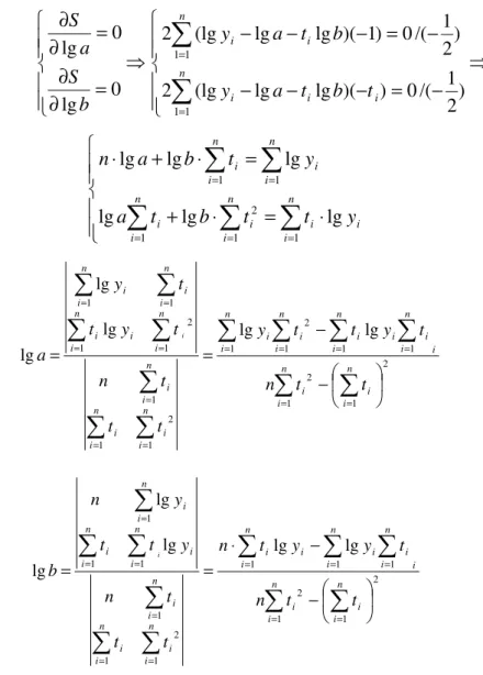
, then the parameters a and b of the adjusted

exponential function, can to be calculated by means of the next system [ ]:

∑

∑

= =

=

−

−

=

⇔

=

−

=

n

i

i i

n

i

t

i

y

S

y

a

t

b

y

S

i

1

2

1

2

min

)

lg

lg

(lg

min

⇒

⎪

⎪

⎩

⎪⎪

⎨

⎧

=

∂

∂

=

∂

∂

0

lg

0

lg

b

S

a

S

⇒

⎪

⎪

⎩

⎪⎪

⎨

⎧

−

=

−

−

−

−

=

−

−

−

∑

∑

= =

n

i i

i n

i i

t

b

t

a

y

b

t

a

y

1 1

1 1

)

2

1

/(

0

)

)(

lg

lg

(lg

2

)

2

1

/(

0

)

1

)(

lg

lg

(lg

2

⎪

⎪

⎩

⎪⎪

⎨

⎧

⋅

=

⋅

+

=

⋅

+

⋅

∑

∑

∑

∑

∑

= =

=

= =

n

i

i i n

i i n

i i

n

i i n

i i

y

t

t

b

t

a

y

t

b

a

n

1 1

2

1

1 1

lg

lg

lg

lg

lg

lg

Thus,

∑

∑

∑

∑

∑

∑

∑

∑

∑

∑

∑

∑

∑

= =

= = = =

= =

= = =

= =

⎟ ⎠ ⎞ ⎜ ⎝ ⎛

− − =

=

n

i

n

i i i

n

i i

n

i i n

i

i i n

i i i

n

i i n

i i

n

i i n

i n

i

i i

n

i i n

i i

t t

n

t y t t

y

t t

t n

t y t

t y

a

i

1

2

1 2

1 1 1 1

2

1 2

1 1

1 2

1

1 1

lg lg

lg lg

lg

and

∑

∑

∑

∑

∑

∑

∑

∑

∑

∑

∑

= =

= = =

= =

= = =

=

⎟ ⎠ ⎞ ⎜ ⎝ ⎛

− − ⋅

= =

n

i

n

i i i

n

i i

n

i i n

i i i

i

n

i i n

i i

n

i i n

i

i n

i i

n

i i

t t

n

t y y

t n

t t

t n

y t t

y n

b

i

1

2

1 2

1 1 1

1 2

1 1 1 1

1

lg lg

lg lg

lg

Table no. 8 The estimate of the value for the variation coefficient in the case of the adjusted exponential function, in the hypothesis concerning the exponential evolution

for the Satisfaction of the Ideal Job in Romania, between 2010-2014

EXPONENTIAL TREND

YEARS

THE SATISFACTI

ON OF THE IDEAL JOB

IN ROMANIA

(%)

(

y

i)

i

y

lg

t

i

lg

y

i

lg

y

ti

=

b

t

a

_i

lg

lg

+

=

ti

ti

ab

y

=

i

t

i

y

y

−

2010 65 , - , , , ,

2011 69 , - , , , ,

2012 70 , , , ,

2013 41 , , , , ,

2014 56 , , , , ,

TOTAL 302 , - , ,

Consequently, if we calculate the statistical data for to adjust the exponential function, we obtain for the parameters a and b the values:

1,75310384 0

10 5

0 ) 340142235 ,

0 ( 10 765519201 ,

8

lg ₂ =

− ⋅

⋅ −

− ⋅ =

a

0,034014223 0

10 5

0 765519201 ,

8 ) 340142235 ,

0 ( 5 lg

2 =−

− ⋅

⋅ −

− ⋅ =

b

%

01

,

14

100

302

298

,

42

100

100

:

exp exp

exp

⋅

=

⋅

=

−

=

⋅

⎥

⎥

⎥

⎥

⎦

⎤

⎢

⎢

⎢

⎢

⎣

⎡

−

=

∑

∑

∑

∑

− = − = −

= −

=

m

m i

i m

m i

t i m

m i

i m

m i

t i

y

y

y

n

y

n

y

y

v

i i

We apply the coefficients of variation method as criterion of selection for the best model of trend. We notice that:

%

01

,

14

%

71

,

12

%

43

,

12

<

=

<

exp

=

=

v

v

v

II I

So, the path reflected by the values regarding the )deal Job in Romania between - , is a parabolic

trend of the shape 2

i i

t

a

b

t

ct

y

i

=

+

⋅

+

, with other words it confirms the hypothesis

H

I .

The type no. 2 The trend model of the values concerning the Satisfaction of the Ideal Job in Romania, between 2010-2014

We observe that, the cloud of points which reflects the values of the Satisfaction for the )deal Job in Romania, between - , it carrying around a quadratic trend model, according to the type no. .

4. The forecasting method regarding the values for the Standard of Living and the Satisfaction of the Ideal Job in Romania

We know that the evolution regarding the Standard of Living in Romania, between - , reflects an exponential trend of the shape i

i

t

t

ab

x

=

:

So, in , the Standard of Living in Romania will be: ₂₀₁₆Romania

=

41

,

7769011

⋅

(

1

,

121785182

)

4

=

66

,

16

%

x

Also, the trend of the values regarding the Satisfaction of the )deal Job in Romania, between - , is a

quadratic trend of the shape 2

i i

t

a

b

t

ct

y

i

=

+

⋅

+

. Thus, in the Satisfaction of the )deal Job in Romania

will be: ₂₀₁₆Romania

=

61

,

25714286

+

(

−

4

,

4

)

⋅

4

+

(

−

0

,

428571428

)

⋅

4

2

=

36

,

80

%

y

.

5. Conclusions

References

1. Gauss C. F. - „Theoria Combinationis Observationum Erroribus Minimis Obnoxiae”, Apud Henricum Dieterich Publising House, Gottingae, 1823.

2. Kariya T., Kurata H. - „Generalized Least Squares”, John Wiley&Sons Publishing House, Hoboken, 2004. 3. Wolberg J. - „Data Analysis Using the method of Least Squares: Extracting the Most Information from