Labor
∗
José Raimundo Carvalho
†
, Emerson Marinho
‡
, Francesca Loria
§
Contents: 1. Introduction; 2. A Benchmark Model of Child Labor; 3. Child Labor and Education; 4. The Data Set Used - Survey of Standards of Living; 5. The Econometric Model; 6. Final Considerations.
Keywords: Child Labor, Multinomial Model, PPV
JEL Code: J13, J47, C25
Although recent trends about child labor are positive, see ILO (2006), there still are important shortcomings which require further investiga-tion. Among them, the exclusion of the category “idle children” (those who neither work nor study) from past studies, as well as the lack of reliable information on returns to education are two significant omis-sions. By using a data base that contains details on idle children and a proxy for the returns to education, we find evidence that confirms traditional findings both with regard to the strong positive effect of pa-rental background and to the positive relationship between the number of children in the household and child labor. On the other hand, our es-timates point out new insights, such as the great regional variation of estimates and the fact that the Body Mass Index effect is positive. Fi-nally, we suggest a new perspective on the issue of “street children” through the analysis of the category of “idle children”.
Apesar das recentes tendências sobre trabalho infantil serem positi-vas, ver ILO (2006), há importantes deficiências no entendimento do fenô-meno. A exclusão da categoria “crianças desocupadas” (não trabalham e nem estudam) em estudos passados, como também a ausência de infor-mações fidedignas sobre retornos da educação são importantes omissões. Utilizando uma base de dados mais detalhada, bem como uma proxy para
∗This paper has been circulated before under the titleSubjective Returns to Education and Child Labor in Brazil, see Carvalho (2004). †I would like to thank the research assistance of Paulo Felipe de Oliveira and Sylvia Lavor, the suggestions of Pedro Ferreira
(EPGE/RJ), Editor of this special issue of the Brazilian Review of Economics, as well as those from two anonymous referees. As usual, any remaining errors are ours. CAEN/UFC, Graduate Program in Economics, Brazil. E-mail:[email protected]
‡CAEN/UFC, Graduate Program in Economics, Brazil. E-mail:[email protected]
§Graduate Student, Barcelona Graduate School of Economics, Spain. I would like to thank the German Academic
retornos da educação encontramos evidências que confirmam resultados tradicionais como o efeito positivo das características dos pais e a relação positiva entre o número de crianças, no trabalho infantil. Por outro lado, apontamos para novos entendimentos, como o fato da variável Índice de Massa Corporal possuir efeito positivo e a grande variação regional dos efeitos das estimativas. Por fim, sugerimos uma nova perspectiva sobre a questão das “crianças de rua” através da análise da categoria de “crianças desocupadas”.
1. INTRODUCTION
According to a recent report from the Director-General of the International Labour Organization, see, ILO (2006), there are good news about the global problem of child labor: child labor is declining, and, the more harmful and hazardous the type of job, the faster the decline. However, citing the same source, child labor is still a pervasive and pressing problem. The Report asserts that the decline was massive in Latin America, so as to“... putting it on a par with some developed and transition economies”.
However, an activity rate of more than5%is not something to be comfortable about.
The issue of child labor is important once one starts thinking about its effects on a child’s psycho-logical and educational achievements, as well as how that kind of activity could impact on child’s future health. In fact, child labor has also deleterious consequences for the whole economy, as it reinforces a sort of “poverty trap” among generations. By forcing their children to work, parents necessarily pre-clude their offspring from the benefits of good education, at least. These children will grow up as bad educated adults which, in turn, will decrease dramatically their chances of getting a good source of income. They will become, than, poor parents, reinforcing the vicious circle of poverty.
In Brazil, the situation has improved after two decades of intensive application of national and local programs to reduce child labor, such as PETI,PETI(National Program for Eradication of Child Labor), andPrograma Bolsa-Escola, (Program of Scholarships). Despite these efforts, there are many issues sur-rounding the determinants of child labor in Brazil. For instance, those programs apparently started without the due scientific scrutiny. Moreover, very few was and is known regarding particularities of how household structure and returns to education affect the amount of child labor. Also, even after all efforts from the federal government, de Barros and de Mendonça (2011) point out that the incidence of child labor is still a pressing problem in Brazil. In particular, they assert that this is due to the fact that the incidence is higher the more vulnerable the socioeconomic group is, up to the point of achieving figures that are four times the national average!
Given this state of affairs, we believe that our main contributions to the literature are threefold. First, we add an important, although underemployed, category of possible “choice” for children to our multinomial logit model of occupational and educational choices: namely, that of idle children (those who neither work nor study). Since a child who neither works nor studies is almost always worse than others who belong to the other three traditional choices (work and study, do not work and study, and, work and do not study), we expect to improve our understanding of child labor issues by decreasing the aggregation of our econometric model. Although this is not the first attempt to stress the importance of considering idle children in empirical implementations of child labor models (see, e.g., Kassouf (2007) and the references provided there), it is the first one backed by an explicitly built model of child labor that admits corner solutions on children’s time allocation (see, Cigno and Rosati (2005)). Also, we believe that the specificities of the data set used are a crucial point of difference between ours and other’s approach.
a proxy for how parents value the education of their offspring, the key question of how to take into account the expectations channel in the context of parents’/children’s decisions is considered more properly. Clearly, this issue plays an essential role in modern theoretical baseline models of child labor as recurrently stressed by Cigno and Rosati (2005).
Third, in order to contribute to the robustness of empirical estimates, an important but rather underused data set is employed: the Pesquisa de Padrões de Vida – PPV. Even though the PPV is far from being an empirical updated snapshot of the current situation of the child labor question in Brazil (currently a data set more than 10 years old), it has unique features as well as advantages compared to the Pesquisa Nacional por Amostra de Domicílio (PNAD) and it portrays the country right at the onset of national programs such asPrograma Nacional de Erradicação do Trabalho InfantilandPrograma Bolsa-Escolawhich were meant, directly or indirectly, to ease the child labor problem in Brazil. This last feature of PPV confers an “historical” advantage over the more recent empirical figures provided, almost exclusively, by the PNAD.
Besides this introductory section, the paper is comprised of Section (2) that builds a necessary survey of the theoretical literature regarding child labor. As outlined above, the literature is so vast that one can easily get lost on his way. Hence, even though a necessary point of departure is the paper of Basu and Van (1998), both because of its originality and conciseness, as well as the seminal approach contained in Baland and Robinson (2000), the chosen starting point is the more modern and comprehensive model of child labor surveyed by means of Cigno and Rosati (2005). The pivotal question of how returns to education affect child labor is the subject of Section (3). Section (4) describes the available data set and outlines its strength and weakness. Because it is a household survey with a sound collection and sampling methodology, it looks strange to us why it is that this data set has not been used more frequently for child labor research. Anyway, the PPV has the strengths of a representative household data set combined with very unique information regarding, especially, education and subject welfare assessments.1 As to the empirical part, Section (5) deals with all the econometric aspects of the paper.
It starts by claiming the adequateness of the multinomial logit model. Subsequently, parameters are estimated by maximum likelihood and the corresponding marginal effects are calculated. A series of specification tests is also performed and its results are discussed. Finally, Section (6) concludes.
2. A BENCHMARK MODEL OF CHILD LABOR
The aim of this section is to provide a modern benchmark model which supports the process of empirically assessing the returns to education in terms of child labor. As simple as this appears, one can soon realize that this is a huge and, indeed, very complicated task. First, the literature can, as we will see, be traced back into the past as deep as to meet some “classical” economists such as Karl Marx, Alfred Marshall and Arthur Pigou. Second, the contemporary literature experienced an enormous boost in the last two decades. Third, there are still so many different potential explanations for this very complex phenomenon that, with no surprise, there is a plethora of different models coexisting. Hence, the next subsection describes the more elaborate and complete approach of Cigno and Rosati (2005), especially as it is concerned with dynamics and fertility decisions.
According to Cigno and Rosati (2005), the following are the main criticisms with respect to past at-tempts to model child labor:2 important model’s implications are very sensitive to initial assumptions,
fertility behavior is crudely modeled, the intertemporal aspects of the problem are addressed in a very basic way, the absence of a more realistic and dynamic trade-off between present consumption and edu-cation. The sensitivity issue can be seen very clearly in Basu and Van (1998) model. Especially regarding
1In fact, there are so many details that we were not able to explore all of the data strengths. This, of course, awaits further
investigations.
2The models of Basu and Van (1998) and Baland and Robinson (2000), albeit they represent important contributions to the
technological postulates, Cigno and Rosati (2005) are incisive in asserting that“... a small change in the technological postulates ... throws doubt on one of the model’s more optimistic implications. The same applies, with greater force, to the representation of parental preferences.” From Basu and Van (1998), one can also notice that the technological assumptions are key to ensure the existence and characterization of the results.
As to fertility behavior, Cigno and Rosati (2005) asseverate that Basu and Van (1998) treat fertility behavior as if parents had perfect control over it. The contradiction, according to them, becomes evident when analyzing the following question: “If it is true that keeping children from working is highest in people’s minds, why is that people have children when the circumstances are such that they will have to work?”. In order to circumvent this problem, Cigno and Rosati (2005) make fertility an endogenous variable. Besides that, fertility is random, which is a much more realistic assumption.
The model appearing in Basu and Van (1998) is a static one. Even though Baland and Robinson (2000) use a two-period overlapping-generation model, it does it inevitably because they will address issues, such as savings and credit constraints, that necessarily demand a dynamical set up. In fact, one of the key contributions of Cigno and Rosati (2005) is to model much more realistically the dynamic aspects of household decisions.
One of the interesting insights gained after two decades of intensive research on child labor is the fact that any candidate for a “good model” of child labor must address the puzzle of “idle” children. Indeed, both Basu and Van (1998) and Baland and Robinson (2000) (and actually almost all predecessors) assume that “education time” is the complement of “working time”. However, the issue is much more complex. As a matter of fact, Biggeri andet alli(2003) show that a large proportion of children who neither work nor study does not do anything.3 Given this, the main contribution of Cigno and Rosati
(2005) is to address partially these concerns by showing that is possible to obtain corner solutions, as well as interior ones, for children time allocation problem between work and school.
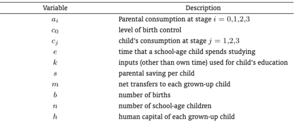
Before getting into details of the model developed in Cigno and Rosati (2005), henceforthCR model, it is essential to understand that a useful model of child labor which assumes a realistic household model, must consider two important issues: the sequential nature of decisions inside the household and the fact that fertility is only partially controlled, i.e., it is a random variable. Cigno and Rosati (2005) start by defining the sequence of decisions taken inside the household. Table (1) describes all the relevant variables. The stages’ decisions and outcomes are:
• STAGE 0
– Along witha0, would-be parents choose the level of birth control,c0. This last variable conditions the likelihood
that a child is born.
• STAGE 1
– This stage comes if and when a child is born. Now, parents decide their own level of consumption,a1, as well as
their child’s consumption (food, attention, medical care, and so on),c1. This last variable conditions the probability
that the child survives up to the next stage.
• STAGE 2
– This stage comes if and when a child survives and reaches school age. Now, parents decidewhether to send their children to school or to work. Also, parents decide their own consumption,a2, as well as each child’s
consumption,c2, time allocated to school,e, inputs used for child education,k, saving,s, and net transfers,m.
Beyond that, children will enter stage 3, as adults, with a stock of human capital,h, and the cycle starts again for a new cohort of adults.
3More specifically, this proportion persists after eliminating those children who perform household chores, who are sick and
• STAGE 3
– This completes the life time of those adults described since stage 0. Now, as old people, they choose their level of consumption,a2, and net transfers,m.
Parents’ preferences are represented by aBecker-styleutility function represented by
U =X
i
ui(ai) +βU∗(c2, y)n, (1)
whereβ ∈(0,1]denotes parents’ altruism towards their children,yis the child’s stage 3 income, and
nthe number of children who live to be adults.
Table 1: Description of Variables
Variable Description
ai Parental consumption at stagei= 0,1,2,3
c0 level of birth control
cj child’s consumption at stagej= 1,2,3
e time that a school-age child spends studying
k inputs (other than own time) used for child’s education
s parental saving per child
m net transfers to each grown-up child
b number of births
n number of school-age children
h human capital of each grown-up child Source:Elaborated by the authors.
One of the significant contributions of theCR modelis to explicitly model the human capital accu-mulation of the children. Accordingly to traditional approaches, they assume that there exists a human capital function that relates innate ability and investment in human capital to the stock of human capital that a child brings to adult life. The function can be written by
h=h0+g(e,k) (2)
whereh0represents natural (innate) talent,echild’s time spent in school andkstands for other
ed-ucational inputs such as books, tuition, transportation costs. It is assumed that the functiong(e,k)
is linear-homogeneous and has constant returns to scale, and thatg(0,k) ≡ g(e,0) ≡ 0. After nor-malizing the time endowment of each child, the cost of providing at least hunits of human capital is
Q(h, wc, pk)≡min
e,k(e wc+k pk), (3)
s.t.h0+h0+g(e,k)≥hand0≤e≤1.
This function is defined for
h≥h0, (4)
they need to decide over the values of(a2, c2, e, k, m, s). In fact, given the cost function (see, equation
(3)), parents choose(a2, c2, h, m, s).
The self-enforcing family constitution is responsible for three constraints4to the parent’s problem.
The first constraint is a consequence of the fact that the family constitution prescribes that parents must give to each of their children, at stage 2, more thanz,
c2+Q(h, wc, pk)≥z. (5)
For the same reason parents, at stage 3, must give back to their adult children some of thexthey are supposed to receive (and actually end up receiving). This is pinned down by the following equation:
x+m≥0. (6)
Finally, defining the interest rate byr, parental old age consumption is determined by
a3=sr−mn. (7)
There are two final constraints. The first one concerns parents’ stage 2 budget constraint:
a2+ [c2+Q(h, wc, pk)]n+s=W2+wcn, (8)
whereW2denotes the sum of the amount, net ofx, due to the grandparents under the family
consti-tution, and of any other fixed charges such as rents or taxes.
The second constraint represents asset and credit market imperfections:
s0≤s≤s1, (9)
where the lower bound,s0, could represent lack of assets to sell or to offer as collateral, and, the upper
bounds1, could represent the usual difficulties in accessing credit markets in developing countries.
Hence, at stage 2, given the number of surviving childrenn, parents solve
max (a2,c2,h,m,s)
U2 = u2(a2) +u3(sr−mn) (10)
+ βU∗(c2, hw+m)n, withβ ∈(0,1]
subject to constraints (4), (5) - (9) and the following “subsistence” restrictions:
a2≥as, a3≥as, c2≥cs, andy−x≥as. (11)
The core of theCR modelwas just described. From this point on, Cigno and Rosati (2005) explore the outcomes associated with equilibria resulting from binding and non-binding restrictions. Since the spirit of our presentation is not to give details of all these results, we hope that the interested reader checks out the original paper to visualize the authors’ many accomplishments.
There are two final contributions from Cigno and Rosati (2005) worth commenting about:5the effect
of access costs and the effect of extreme poverty on child labor. As to the effect of access costs on child labor, Cigno and Rosati (2005) offer a interesting explanation for the existence of a large proportion of children reporting doing nothing (i.e., idle children) in surveys. Regarding the effects of extreme poverty on child labor, the authors explain that income has a stronger effect the closer the family stands in relation to some poverty line metric. This result, of course, has important policy prescriptions. Next section describes a key aspect that is intrinsically related to child labor: education.
4These constraints are not necessarily binding. It could happen that some of them could be binding at the same time. 5It is important to mention a deliberate omission of our survey. The fertility issue, although receiving a whole chapter of Cigno
3. CHILD LABOR AND EDUCATION
For a good understanding of the relationship between child labor issues and education it is sensible, firstly, to have a closer look at what one means by the term education. From the perspective of child labor studies such as Cigno et al. (2006) and Edmonds (2008), the term education can have, depend-ing on the context, different meandepend-ings. It could mean educational outcomes such as grades, learndepend-ing achievements, highest academic degree and so on. It could mean the returns to education, i.e., how much a person could improve its well-being by acquiring additional schooling. In this context, the liter-ature is looking for a causal effect of returns to education on child labor. Finally, it could mean parents’ educational background and how this influences (their) choices of children’s working time.
Whatever the context under review, the subject is surrounded by empirical and theoretical diffi-culties. For instance, returns to education is a concept sometimes hard to define and, especially, to quantify. Given the complexities of the subject, we start by describing contributions that try to identify an effect of child labor on educational outcomes.
3.1. The Effect of Child Labor on Educational Outcomes
According to Edmonds (2008)“the extent to which work affects schooling performance , and attainment is perhaps the second most researched question in the child labor literature.” Indeed, the modern literature on the consequences of child labor on educational issues is large, as can be seen in Orazem and Gun-narson (2004). To start understanding how to interpret this problem, it is an interesting strategy to build up a conceptual framework. Hence, we will closely follow the approach appearing in Orazem and Gunnarson (2004).
Orazem and Gunnarson (2004) utilize a variant of the classic model appearing in Ben-Porath (1967). The proposed model has the following characteristics:
1. The path from childhood up to the end of adulthood is aggregated into three periods of time. The first stage is defined as the length of time a child spends all of his/her time at school, i.e.,A= 1. The second stage is where parents decide whether their children will spend any time working. So, at this stage,A∈(0,1). In the third and final stage the child specializes in working, meaning thatA= 0and, consequently,L= 1.
2. Parents decide the allocation of their children’s time between labor and school attendance.
3. The returns to education are assumed to be positive and decreasing with years of schooling. The wage a worker child will receive at timetis given by: W(Ht), whereHtis the total human capital accumulated att.
Assuming an exogenous interest rate r, a straightforward “cut-off” rule can be represented by the following equilibrium condition6
−AW(H0) +W(H1)−W(H0)
1 +r ≥0. (12)
The interpretation of this condition is well known: the child should attend school if the present value of an additional unit of time studying is greater than the cost of acquiring this additional unit of time. In fact, this is a traditional outcome of human capital accumulation models. Interestingly, because the returns to education are assumed to be diminishing with schooling years, the traditional life-cycle of time allocation is obtained, i.e., initially people only study (A = 1), then, do both schooling and working simultaneously (A∈(0,1)andA+L= 1) and, finally, people only work (A= 0andL= 1).
As simple as it appears, the result above is just one side of the problem. Remember that the proposed agenda is to investigate the impact of child labor on educational outcomes. Thus, it is necessary to incorporate an educational production function into the framework. Orazem and Gunnarson (2004) conjecture the existence of a production function of the following form
Hij=H(Cij, Zj, Hij0), (13)
where i and j respectively index the child and the household. Cognitive attainment (as measured by test scores) is represented by Hij, Zj is a vector of variables thought to have an impact on the production of human capital (parents’ attributes, community’s characteristics, etc.) and Hij0 is past schooling and/or unobserved ability. The educational production function “closes” the model. Hence, the channel through which child labor affects educational outcomes is obtained by putting together equations (12) and (13).
In order to have a glimpse on the available empirical results, we briefly comment on a couple of papers. As outlined before, Ravallion and Wodon (2000) find that an increase in child labor is not associated with changes in school enrolment in Bangladesh. This leads the authors to conclude that the effect of child labor on school enrolment, if it exists, is probably small. However, Orazem and Gunnarson (2004) draw attention to the fact that this apparent lack of association between child labor and school enrolment could be masking an undesirable phenomenon: children could be adjusting the changes in time devoted in child labor at the intensive margin, i.e., they remain enrolled but do not attend school as regularly. This was exactly the result obtained in Boozer and Suri (2001) who conclude that in Ghana an one hour increase in child labor reduces school attendance by 0.38 hours. As to school achievement, there is evidence that child lowers years of attained schooling, see for instance Psacharopoulos (1997). However, the study is open to methodological criticism by not controlling for endogeneity of child labor. Studies that attempt to correct the endogeneity are Rosati and Rossi (2001) and Gunnarsson (2003). These two studies find again the deleterious effects of child labor on school achievement but this time, possibly due to the correction of endogeneity, they are smaller. Although the study of the effects of child labor on educational outcomes is a very important issue, it would bring us too far from our initial objective. This means, one should try to discuss how returns to education, broadly defined, affect child labor. This is the subject of the next subsection.
3.2. How Returns to Education Affect Children’s Time Allocation?
There is a large body of literature that explicitly shows the link between returns to education and child labor. Indeed, both models discussed before, i.e., Baland and Robinson (2000) and Cigno and Rosati (2005), make use of the return of education. The present section discusses two interrelated issues: which variables are relevant in the context of returns to education, and by which mechanism returns to education influence child labor. But before that, the effect of parents educational background on child labor is briefly discussed.
Regardless of what is the explanation for asymmetries between fathers and mothers, it is a reality that the role mother’s education plays in child labor issues has been recognized by policy makers. An interesting example is the fact that programs aiming to reduce child labor by means of conditional cash transfers, for instance PROGRESA in Mexico and BOLSA ESCOLA in Brazil, elect the mother as the recipient of the money. This clearly acknowledges the fact that mothers “care” more about their children.
The traditional approach related to time allocation and human capital investments is grounded in the seminal contributions of Gary Becker, for instances, Becker (1965) and Becker (1991). As outlined in the models of Baland and Robinson (2000) and Cigno and Rosati (2005), by solving an optimization problem, parents must decide how much time their children must devote to each of the competing tasks. For ease of explanation, let us assume that children’s available time should be allocated between two non-overlapping and exhaustive tasks: work and school. Now, according to the tenets of the neoclassical approach, parents have to take the following decision: How much timet∗
wshould my child
work? Clearly, by choosingt∗
wthe parent is also choosing the amount of time his/her child will spend
in school,t∗
s, via the available time constraint.
Now, for each additional fraction of time the parent is willing to devote to/diminish from child labor
∆t∗
w(or, equivalently, to remove from/devote to child schooling), he/she will have a marginal loss/gain.
The marginal gain can be understood as the improvement7in the parent’s well being arising from the
fact that his/her child will have a greater amount of schooling. Obviously, these gains in welfare are consequence of higher wages for his/child and/or of altruistic considerations. Anyway, one can put all marginal gains in terms of increased parental utility under the same tag and call it returns to education. As it will be clear next, a better name would be “gross return to education”. Now, along with the gains originated by greater time devoted to schooling, there will be associated costs.8 Thus, an increase in
time devoted to schooling will require additional costs. The returns to education net these additional costs would be better called “net returns to education”.
The line of reasoning is then that parents will increase their offspring’s schooling time if, and only if, the “gross return to education” is greater than the associated marginal costs or, in other words, if the “net returns to education” are positive. This adjustment process ceases when “net returns to education” are equal to zero. The mechanism through which returns to education influence child labor decisions is than by the impact that these decision have on parents’ well-being. This and the preceding section concluded the necessary theoretical explanation for the understanding of the modern debate about child labor, with special emphasis on education. Next section deals with the chosen methodology, describes the data set used and performs important preliminarily empirical analysis.
4. THE DATA SET USED - SURVEY OF STANDARDS OF LIVING
The “Pesquisa sobre Padrões de Vida” (PPV), Survey of Standards of Living, was a major effort taken by the Brazilian government jointly with the World Bank aiming at gathering a comprehensive data set in order to quantify and identify the determinants of the well being of the population as well as assess the impact of public policies and programs. The PPV was a pilot project and it was conducted during the period of 1996-1997. As a specific goal, the PPV wanted to put together a set of information concerning household components’ well-being that used to be found only if one looked for different data bases.
Before we turn to the details of the data set, it is worth stressing two essential aspects of the PPV. First, the data set has labor market information from people with ages as early as 5 years. Clearly, this is
7From this point on, we are doing our thought experiment by assuming that∆t∗
w<0, i.e., the parent is increasing the time of
the child’s schooling. The effect of∆t∗
w>0is completely analogous.
a key feature as we are interested in studying child labor. Second, there are enough details on children’s time allocation as to permit us to depart from past analysis that assumes only the dichotomy work
versusschool. A final remark is important: even though there is a huge lively debate over the right definition of child labor, we just follow “traditional” approaches and define child labor as it appears in, e.g., Cigno and Rosati (2002) and Cigno and Rosati (2005). This means that we made a “cut” in our sample and considered as child workers all children from 6 (inclusive) up to 16 (inclusive) who responded that had a work in the last seven days. At this point, we are able to start analyzing and comparing9our data set.
Table (2) shows the distribution of children, by sex, among four mutually exclusive activities: work only, neither work nor study, study only, and, work and study. A first striking result is the fact that, even by the end of the20thcentury,13.72%of children are laborers (work only or work and study). For
rural India this number goes to14.52%. Also, boys work and study twice as much as girls.
Table 2: Work/study status of children by sex (%)
Male Female All
Work only 4.47 2.11 3.32
Neither Work Nor Study 7.11 9.20 8.13
Study only 74.46 82.04 78.15
Work and Study 13.96 6.65 10.40
Source:Elaborated by the authors, from PPV.
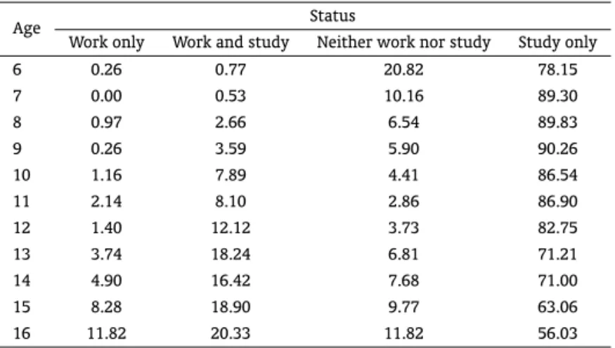
Table (3) shows the distribution of activities by age group. If we start reading the Table by going down in the “Work only” column a pattern of increasing percentage of people engaged in work can be becomes apparent. More specifically, the greatest marginal increase takes place from15to16years. This pattern also occurs in the “Work and study” column. As to the column “Neither work nor study”, it must have brought a bad and alarming picture for scholars and policy makers at that time. Its “U” shaped representation, i.e., starting with20.82%, achieving a minimum at11years with2.86%, and, finally going up to11.82%must have been quite bad news.
Table 3: Work/study status of children by age (all) (%)
Age Status
Work only Work and study Neither work nor study Study only
6 0.26 0.77 20.82 78.15
7 0.00 0.53 10.16 89.30
8 0.97 2.66 6.54 89.83
9 0.26 3.59 5.90 90.26
10 1.16 7.89 4.41 86.54
11 2.14 8.10 2.86 86.90
12 1.40 12.12 3.73 82.75
13 3.74 18.24 6.81 71.21
14 4.90 16.42 7.68 71.00
15 8.28 18.90 9.77 63.06
16 11.82 20.33 11.82 56.03
Source:Elaborated by the authors.
Indeed, this feature of the data set deserves much more concern as one starts conjecturing about what those kids are doing. They are probably wandering around the big cities of Brazil begging, committing small crimes and, likely, preparing themselves to be criminal adults.10
Nevertheless, for as ironic as it could be, Brazil is much better off than rural India because, for all age groups, the percentage of people doing nothing in India is almost twice the percentage for Brazil (see, Cigno and Rosati (2005), pp. 85). Tables (4) and (5) show the distribution of activities by age group for boys and girls, respectively. The patterns are roughly the same, the column “Neither work nor study” presents, again, the “U” shaped form.
Table 4: Work/study status of children by age (boys) (%)
Age Status
Work only Work and study Neither work nor study Study only
6 0.53 1.05 22.11 76.32
7 0.00 0.51 10.26 89.23
8 1.38 3.69 5.99 88.94
9 0.51 5.10 4.59 89.80
10 2.22 11.11 5.78 80.89
11 3.00 10.73 2.15 84.12
12 1.73 15.15 3.03 80.09
13 5.22 24.35 4.78 65.65
14 4.80 22.71 6.11 66.38
15 11.84 25.31 7.76 55.10
16 16.92 28.86 8.46 45.77
Source:Elaborated by the authors.
Table 5: Work/study status of children by age (girls) (%)
Age Status
Work only Work and study Neither work nor study Study only
6 0.00 0.50 19.60 79.90
7 0.00 0.56 10.06 89.39
8 0.51 1.53 7.14 90.82
9 0.00 2.06 7.22 90.72
10 0.00 4.37 2.91 92.72
11 1.07 4.81 3.74 90.37
12 1.01 8.59 4.55 85.86
13 2.22 12.00 8.89 76.89
14 5.00 10.42 9.17 75.42
15 4.42 11.95 11.95 71.68
16 7.21 12.61 14.86 65.32
Source:Elaborated by the authors.
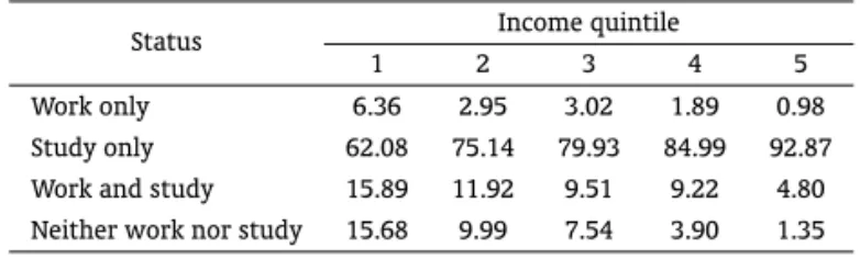
The fact that income is a key determinant of child labor is a recurrent topic in the literature. In fact, as outlined before, income has a direct effect as well as an indirect effect. The direct effect is
10One of the referees pointed out that the percentage of children who “Neither work nor study” (idle children) was high because
represented by the fact that the lower the income, especially if the household is getting closer to the subsistence level, the more parents are forced to diminish any altruistic feelings and to supply more of their children’s available time. The indirect effect, examined in the seminal paper of Baland and Robinson (2000), is due to credit constraints. Since credit constraints are highly prevalent among the poor or very poor, income has an indirect effect on child labor too.
Table 6: Work/study status of children by household income (%)
Status Income quintile
1 2 3 4 5
Work only 6.36 2.95 3.02 1.89 0.98
Study only 62.08 75.14 79.93 84.99 92.87
Work and study 15.89 11.92 9.51 9.22 4.80
Neither work nor study 15.68 9.99 7.54 3.90 1.35 Source:Elaborated by the authors.
Two patterns are worth commenting in Table (6). First, it is evident that income is highly correlated with child labor, i.e., the lower the income quintile the greater the percentage of children who only work. The category “Neither work nor study” features the same pattern. Moreover, there is a strong correlation between the “Study only” and income quintile: the higher the income quintile the greater the percentage of children who only study.
Summing up, the PPV seems to offer a very rich and interesting data set to explore the determinants of child labor. Especially regarding education, the PPV has a reasonably detailed set of information. This type of information goes beyond the tradition of only reporting some proxy for educational attainment. The data brings detailed event-history type of information about the educational prospects of all in-dividuals from the sample. Next section is concerned with developing and estimating an econometric model of child labor. As it will be shown below, we are able to reasonably accomplish this objective using a multinomial logit model and applying it to a subset of the PPV data set.
5. THE ECONOMETRIC MODEL
Econometric models trying to assess the impact of different variables on the time children allocate to different tasks have been estimated for a couple of years. Modern examples are Deb and Rosati (2002), Ray (2000), Cigno and Rosati (2002), and, Cigno and Rosati (2005). The literature applying these models to Brazil is much less representative, however. Good examples are Kassouf et al. (2001), Kassouf (2007) and Soares et al. (2012). With few variations, these authors apply a set up that treats the choice of different tasks as an outcome from a set of finite alternatives and employ multiple choice models (almost always multinomial logit).
passed and sanctioned the Programa Bolsa Escola11(see, Denes (2003)). The next two subsections deal
with the multinomial logit model and the estimation process, respectively. First, a concise discussion of the multinomial logit model and how it incorporates the issues surrounding child labor is developed. After that, estimations are performed and the model’s outcomes are analyzed.
5.1. The Multinomial Logit Model
Our empirical model, although not belonging to the “structural” approach, considers an underlying conceptual framework that was described by the models of Basu and Van (1998), Baland and Robinson (2000), and, Cigno and Rosati (2005). Parents are assumed to control their children’s time endowment and to choose among four different and exhaustive alternatives, namelywork only,school only,work and schoolandidleness.
The theoretical models described support the existence of a latent parent utility index. As it became conventional in the literature of discrete choice (see, e.g., Wooldridge (2002)), this latent random vari-able is calledindirect utility function. Hence, we assume that a parent from a specific household will choose for childi, the occupationj, wherej= 0,1,2,3if he/she will choose the alternativework only,
work and school,idlenessandschool only, respectively. The parent’s indirect utility function then is:
y∗ij=X′β+ǫij, (14)
whereyij∗ is the indirect utility function,Xis a vector of independent variables thought to influence the parent’s choice,βis a vector of correspondent parameters andǫijis a unobserved random error whose distribution is assumed to be Weibull. Now, the maximizing behavior of parents yields the following result: A given parent whose vector of independent covariates isXwill choose alternativek= 0,1,2,3
for his/her child if, and only if, this alternative gives him/her the highest value for indirect utility. This means that:
P rob(yi=k|X) =P rob(yik∗ ≥y∗i0, y∗ik≥y∗i1,· · · , y∗ik≥yi∗3), (15)
whereP rob(yi =k|X)represents the probability that theithparent choose that his/her child should
perform taskk. Clearly, from Equation (15), the value ofP rob(yi = k|X)requires the calculation of
multiple integrals. This notwithstanding, a straightforward result from the literature on discrete choice asserts that ifǫijare Weibull, the formula for multinomial logit probabilities becomes:
P rob(yi=k|X) = exp(X
′β+ǫik)
P3
j=0exp(X′β+ǫij)
, (16)
wherek= 0,1,2. Assuming that observations are independent among households and children inside a household, maximum likelihood can be directly applied to the sample. Note, however, that as sim-ple as it appears, the multinomial logit model has two caveats worth mentioning. First, there is the famous implicit assumption of Irrelevance of Independent Alternatives (IIA). A second issue regarding the multinomial logit model is the fact that the marginal effects of estimated parameters are compli-cated to calculate. One can not infer from estimated parameters the values of the marginal effects, i.e.,
∂P rob(yi|X)
∂xi , wherexi is a specific continuous covariate included in the random vectorX. However,
most econometric and statistical packages have routines to calculate that, in our case ST AT AT M
(see, StataCorp (2009)). Next subsection describes the chosen explanatory variables and performs esti-mations based on the multinomial logit model.
5.2. Estimation
We start by describing the variables that appear in Table (7). In order to have a general picture of the available empirical content, this table lists all variables used as well as some descriptives statistics. The variablesextries to capture any difference between parents’ behavior towards their children’s sexes. There has been empirical support for the fact that parents tend to invest more in males(see, Cigno and Rosati (2005)). We also control for race although the concept is unlikely to be important giving the well known Brazilian historical miscegenation process. Age effects are captured by bothageandage2
(age squared), with the latter trying to represent any non-linear effect of age. The important variable
education, measures the completed years of education of the child. Clearly, this is an important control as one expects the probability of sending a child to work to decrease the highereducationis,ceteris paribus.
Both the number and age structure of the household’s children are represented by the variables
n6−16andn0−5; respectively, the number of children aged between six and sixteen years, and, the number of children aged between zero and five years. The justification for the use of such type of variables dates back to the seminal paper of Becker (1965) on child’s investment by parents. Also, these variables’ use is rooted on fertility issues that appear in, for instances, Basu and Van (1998) and Cigno and Rosati (2005). The “quality” of children is proxied by the variableBM I, Body Mass Index. The BMI is a widely used index to measure nutritional status of human population. Especially in economics, the BMI has been used not only to measure nutritional status but also as a good predictor of children’s survival to subsequent stages of life (see, for instance, Klasen (1996)).
Table 7: Description of Variables and Descriptive Statistics
Variable Description Mean Std. Dev. Min Max Obs
sex child’s sex (male = 1) 0.51 0.50 0 1 4664
race child’s race (white = 1) 0.41 0.49 0 1 4664
age child’s age in years 11.18 3.14 6 16 4664
age2 squared child’s age in years 134.89 69.81 36 256 4664
education child’s education in years 3.75 2.53 1 12 4664
n6-16 number of children (6≤age≤16) in the household 2.52 1.35 1 8 4664
n0-5 number of children (age≤5) in the household 0.51 0.82 0 5 4664
BMI BMI (height2weight) 18.09 3.47 9.13 43.04 4340
northeast regional dummy (NE = 1) 0.58 0.49 0 1 4664
urban geographical dummy (urban = 1) 0.71 0.45 0 1 4664
educf father’s education (elem. = 1, middle = 2, 1.80 0.99 1 4 3629
high = 3, superior = 4)
educm mother’s education (elem. = 1, middle = 2, 1.79 0.97 1 4 3818
high = 3, superior = 4)
size number of people in the household 5.75 2.24 2 16 4664
income household income per capita 285.38 585.36 0 13361.81 4346
eval. subjective welfare question (very good = 1, good = 2, 2.73 0.87 1 5 4649 regular = 3, bad = 4, very bad = 5)
status_child child’s status (work only=1, work&study=2, 3.61 0.80 1 4 4664 neither work nor study=3, study only=4)
Source:Elaborated by the authors.
and most developed region of Brazil. As a matter of fact, the state of São Paulo, the richest and more industrialized in the whole country, is located in the Southeast region. Differently, the Northeast region has been historically a very poor and unequal place. These regional differences are captured by the dummyregion.
The geographical area can be inferred from the dummyurban. That child labor could have different determinants if the analysis was performed in urban areas or rural areas is a point already known to researchers. For this reason, it is very important to condition on that variable. Indeed, it appears that the very type of job which children perform in rural areas is different than the type of tasks performed by urban children. For instance, while it is more likely that a rural child laborer performs agricultural tasks (which is presumably less deleterious to his/her health) a urban child worker is probably doing a harder job. Also, idleness in urban areas raises much more concerns than its reciprocal in rural areas.
As discussed in Subsection (3.2), parents educational background is likely to influence child labor. These influences are not symmetrical, as past studies12show that mothers will probably have a stronger
effect than fathers do. The two variables,educfandeducmrespectively represent father’s educational achievement and mother’s educational achievement. The size of the household is represented bysize
and includes all household members, namely parents, children, grandparents and servants. Income
per capitais used as a measure of available resources to spend in consumption. Of course, one might wonder why measures of wealth were not applied. There are a couple of variables in PPV that could be used as proxies for wealth. However, the number of missing values is huge. The variableincome
is used to represent incomeper capita. The last variable,eval., measures the expectation that parents have over their children’s level of education. For this kind of variables, as far as we know, has not appeared in the literature of child labor, it deserves a little elaboration.
Before we proceed to discuss estimations results,13this is a nice point to comment about
endogene-ity issues and how we have dealt (in fact, avoided it) with that econometric problem. Of course, as simple as the estimable model of child labor could be, it is almost impossible to get rid of endogenous variables by construction. We are well aware of many sources of endogeneity and just to simplify the discussion we are in agreement with both referees and the Editor regarding the variables that measure children schooling and BMI. In fact, we could offer other examples of endogenous variables that pop up on child labor models and, more specifically, in our own model. However, the reason for not trying to control for that is grounded on pragmatism: addressing endogeneity issues in multinomial models (ordered or unordered) is far from being settled and it will send us far from the original scope of our investigation.
There are basically three ways to control for endogeneity in multinomial models: i) by approach-ing the problem from a maximum likelihood point of view, ii) by usapproach-ing “control functions” and iii) by estimating a linear probability model. All three approaches have serious drawbacks and only in very special cases they could turn into a reasonable and competitive option. Dong and Lewbel (2010) made that point very clear. In order to corroborate our pragmatism, we would like to end up this discussion by calling the attention that even very new results on estimation of multinomial models of child labor, see Soares et al. (2012), refrain from a “direct” approach to endogeneity. Past studies either refer tan-gentially or just do not even mention the issue. We proceed now to discuss the inclusion of parents’ expectations over their children’s education into the model.
As a nice innovation, the PPV, in Section 15 -Avaliação das Condições de Vida (Evaluation of Life Conditions), makes some subjective welfare measurement questions. These kind of questions ask the household member to answer his/her subjective assessment of welfare in different situations. Some-times it could ask, for instance,
12See those citations at Subsection (3.2).
13After eliminating missing observations, the remaining sample contained 2,903 observations. Nothing indicates that the
In your opinion, the total income of your family allows that all of you live your lives?: with difficulty, more and less difficulty, or, easily.
Another question asks the respondent to grade, in a subjective scale, how he/she evaluates some di-mensions of household welfare or expenditures. For example,
How do you evaluate the life conditions of household members regarding to Education/Schooling Level?: very good, good, regular, bad, and, very bad.
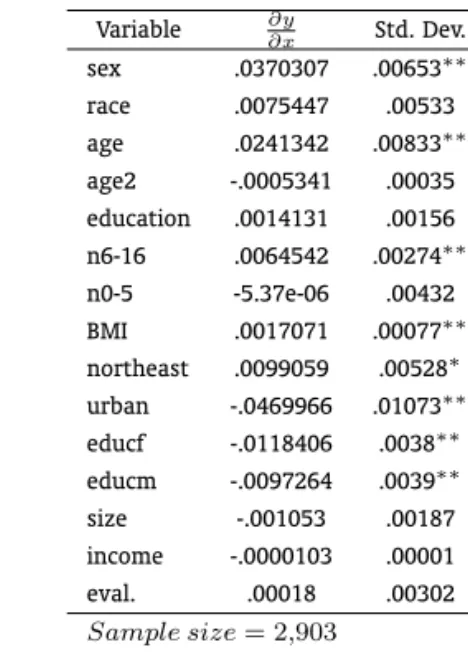
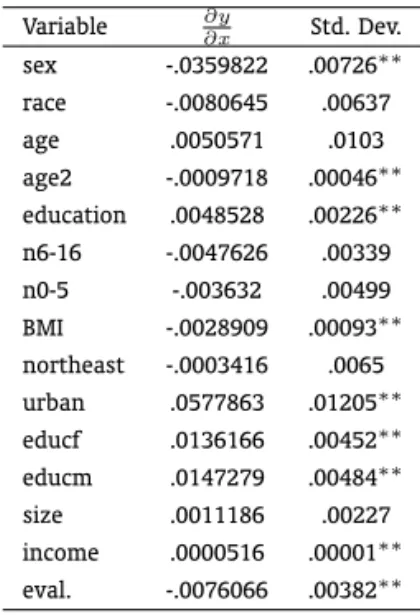
The latter was the exact question that we have taken in order to use it as the last independent variable. The hope is that this variable, represented by eval., could be an exogenous source of variation of how intense the household head values the level of schooling of the household members. It is a first innovative attempt to depart from traditional measures of returns to education that are so hard to figure out. The use of subjective questions to aid the estimation of econometrics models is a roughly recent development, (see, for instances, Pradhan and Ravallion (2000), and, van Praag et al. (2000)). The next step is to estimate the model. The adopted model is described in Equation (16). Tables (8), (9), (10) and (11) represent the marginal effects foronly work,work and school,idleness, and,school only, respectively.
Table 8: Effects - (Only Work)
Variable ∂y∂x Std. Dev.
sex .0009112 .00059
race -.0002638 .00029
age -.0004167 .00058
age2 .0000399 .00003
education -.0003051 .0002 n6-16 -.0000915 .00012
n0-5 -.0001755 .00022
BMI .0000284 .0004
northeast -.0006199 .00046 urban -.0053117 .00329∗
educf -.0008157 .00044∗
educm -.0000219 .00028
size .0001126 .0001
income 3.68e-07 .00000∗
eval. .0002189 .00019
Sample size= 2,903
*p <0.1, **p <0.05
Table 9: Effects - (Work and Study)
Variable ∂y∂x Std. Dev.
sex .0370307 .00653∗∗
race .0075447 .00533
age .0241342 .00833∗∗
age2 -.0005341 .00035
education .0014131 .00156 n6-16 .0064542 .00274∗∗
n0-5 -5.37e-06 .00432
BMI .0017071 .00077∗∗
northeast .0099059 .00528∗
urban -.0469966 .01073∗∗
educf -.0118406 .0038∗∗
educm -.0097264 .0039∗∗
size -.001053 .00187
income -.0000103 .00001
eval. .00018 .00302
Sample size= 2,903
*p <0.1, **p <0.05
Before we start commenting on the estimated coefficients, it is important to describe more carefully the interpretation of the results. To do so, note that:
1. All marginal effects are calculated having the choiceStudy only as the referential state. This means that any draw conclusions must consider that;
Table 10: Effects - (Neith. Work nor Study)
Variable ∂y∂x Std. Dev.
sex -.0019598 .00292
race .0007836 .00315
age -.0287747 .00604∗∗
age2 .0014661 .0003∗∗
education -.0059609 .00153∗∗
n6-16 -.0016001 .00176
n0-5 .0038128 .00223∗
BMI .0011554 .00048∗∗
northeast -.0089444 .00347∗∗
urban -.005478 .00422
educf -.0009604 .00237
educm -.0049797 .00283∗
size -.0001782 .00112
income -.0000417 .00001∗∗
eval. .0072078 .00218∗∗ Sample size= 2,903
*p <0.1, **p <0.05
Table 11: Effects - (Study Only)
Variable ∂y∂x Std. Dev. sex -.0359822 .00726∗∗
race -.0080645 .00637
age .0050571 .0103
age2 -.0009718 .00046∗∗ education .0048528 .00226∗∗
n6-16 -.0047626 .00339
n0-5 -.003632 .00499
BMI -.0028909 .00093∗∗
northeast -.0003416 .0065 urban .0577863 .01205∗∗
educf .0136166 .00452∗∗
educm .0147279 .00484∗∗
size .0011186 .00227
income .0000516 .00001∗∗
eval. -.0076066 .00382∗∗ Sample size= 2,903
*p <0.1, **p <0.05
After these initial remarks, let us proceed to the analysis. The first interesting point is the fact that for those variables that have a significant parameter, the absolute values forWork and Studyare greater than those values forOnly Work. This is the case forsex,age,n6−15,BM I,northeast,
urban,educf andeducm. A likely explanation is that the stateOnly Workis a quite awful one. Even in poor households, the availability of information about the risks associated with child labor refrains parents to condemn their children to such a terrible situation which translates on estimated parameters with lower marginal elasticities. However, the stateWork and Studyis much more sensitive to changes in independent variables; sometimes more than ten times the correspondent effect.
Continuing onWork and Study, it is important to first note the great impact of the variableurbanin the probability of belonging to that category. The key interpretation problem is that for a given effect, say an increase in the probability of Work and Study, one may wonder whether the improvement happens because more people who used to work only started to study also, or whether people who only studied started to work altogether.
The effect of parents’ educational background is both negative (the higher parent’s education the lower the amount of children on this state) and significant. Interestingly, the impact of fathers is greater than that of mothers’. Now,ageandage2are positive and negative, respectively. This means that the older the child the less likely it is that he both works and attends school. However, this pattern is not monotonic; it reaches a maximum than decreases sinceage2 =−.0005341. Also, BMI is now positive and significant, showing probably that parents will allow better nurtured children to do some working besides going to school. The variablesincomeandevalhave the expected values, i.e., negative and positive, respectively, even though neither are statistically significant. Finally, it is worth mentioning that the number of children aged between six and sixteen has a positive effect. Probably, the greater the number of children the higher the probability a parent will send their children to work as a supplemental income device.
ForOnly Work, it is important to stress the fact that no parameter is significant at a5%level. The only parameters significant at a10% level (sometimes borderline significant) areurban,educf and
although the value is not different from zero. This apparently contradictory result could be reflecting credit constraints. The urban dummy points out that children living in urban areas have a lower chance of belonging to theOnly Work category. It is also important to note that the positive sign ofeval.
makes sense, meaning that the higher the value of this variable the lower the chances of child labor. However, the parameter is not significant. We move on to discuss the key category ofNeither Work nor Study, henceforth “idle children”.
With regard to “idle children”, it is not a surprise to see that the higher mother’s education, child’s education and income per capita, the lower the probability of belonging to this set of children. A fact worth stressing is that the elasticity of income is comparable in absolute value (actually, quite similar) only to the other “extreme” case ofStudy Only. It is almost2,000and700greater than those figures of the categoriesOnly WorkandWork and Study, however. This high elasticity of income offers some clues as to how slightly additional sources of income to the household could ease the deleterious problem of “idle children”.
Who are those “idle children”? Can we conclude that “idle children” and “street children”14are the
same set? Although we do need much more investigation into those issues to have any reasonable answer, the variableBM Ibrings up to the surface an interesting hint.
For “idle children”,BM Ihas a positive sign. This is so despite the fact that those children belong with a very high probability to the lowest income quintile (see, Table 6). So, a child lives in a very poor household and a marginal increase in his/her BMI increases the chances of becoming idle. We rationalize such kind of effect as meaning that stronger children in extremely poor households can survive and get money on the streets,caeteris paribus. Thus, we tentatively suggest that, at least, the set of “idle children” and the set of “street children” have some important intersections. Of course, endogeneity must have a bite here. Furthermore, note that the fact that the parametersexis negative (−0.0019) and statistically significant is at odds with our interpretation. The next Section concludes by commenting on some issues that could be discussed taking the estimates in consideration.
5.3. Specification Analysis
In this section, we are going to discuss the adequacy and accuracy of the multinomial logit model. Following Loria (2012), we apply a series of specification analysis in order to test the model fit and accuracy. Table 12 reports, inter alia, six important indicators which we will briefly comment on.
We begin with the p-value of the Likelihood Ratio (LR) Chi-Square test (Prob>chi2). It tests whether for all three equations (Work OnlyversusWork and Study,Work OnlyversusNeither Work nor Study,
Work and StudyversusNeither Work nor Study) at least one of the predictors’ regression coefficients is not equal to zero. This null hypothesis can be rejected at every possible significance level if the p-value is equal to zero, which is precisely the case here.
We proceed with some goodness-of-fit measures represented by their Pseudo-R2. Differently from the “normal” one, they do not reveal the proportion of the dependent variable variance explained by the predictors. For instance,McFadden’s and Cox-Snell’s Pseudo-R2indicate to which extent the full model offers improvement in terms of likelihood over the intercept model by comparing their ratio. The smaller the ratio, the better the fit of the full model compared to the intercept model. McFadden’s Pseudo-R2can lay between zero and one with values in the range of 0.2 and 0.4 suggesting a very good fit. Note that Cox-Snell’s Pseudo-R2has a maximum value of 0.75.
Further fit measures are the well knownAkaike(AIC, AIC∗N) andBayesian(BIC, BIC’)information criteria. These come in handy in the model selection process and are thus only reported to facilitate
14This is a very popular denomination for those children from extremely poor households that spend almost the whole day
Table 12: Model’s Performance Indicators
Log Likelihood -1135.134
LR chi2(45) 856.392
Prob>chi2 0.0000 PseudoR2(McFadden) 0.274
Adj. PseudoR2(McFadden) 0.233 PseudoR2(Cox & Snell) 0.2555
Information Criteria
ll(null) -1563.330
ll(model) -1135.134
degrees of freedom (df) 45
AIC 0.826
AIC∗N 2398.269
BIC -20366.498
BIC’ -497.584
Classification of Cases Percentage of correctly
predicted results 78.07%
Source: Elaborated by the authors.
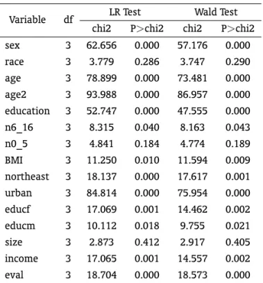
Table 13: Tests for Independent Variables
Variable df LR Test Wald Test chi2 P>chi2 chi2 P>chi2 sex 3 62.656 0.000 57.176 0.000 race 3 3.779 0.286 3.747 0.290 age 3 78.899 0.000 73.481 0.000 age2 3 93.988 0.000 86.957 0.000 education 3 52.747 0.000 47.555 0.000 n6_16 3 8.315 0.040 8.163 0.043 n0_5 3 4.841 0.184 4.774 0.189 BMI 3 11.250 0.010 11.594 0.009 northeast 3 18.137 0.000 17.617 0.001 urban 3 84.814 0.000 75.954 0.000 educf 3 17.069 0.001 14.462 0.002 educm 3 10.112 0.018 9.755 0.021 size 3 2.873 0.412 2.917 0.405 income 3 17.065 0.001 14.557 0.002 eval 3 18.704 0.000 18.573 0.000
Ho: All coefficients associated with given variable(s) are 0.
comparisons with other models. Please refer back to theST AT AT Mfitstatdocumentation file for more details (see also, Long and Freese (2006)). Another evaluation method we consider is the classification table. First, probabilities are assigned to each state of the dependent variable and the one which has the highest probability is selected to be the actually predicted outcome. Then, the observed values of the dependent variablestatus_childare compared with the predicted ones. In this way, it is possible to calculate thepercentage of correctly predicted resultswhich, in this case, amounts to 78.07%.
It is well known that the inclusion of irrelevant variables usually results in coefficient bias and poor model fit. Valid tools to test the significance of each independent variable are the Likelihood-ratio (LR) and the Wald test (Table 13). To carry out these tests we used the postestimation commandmlogtestin
ST AT AT M (see, Long and Freese (2006)). The LR test reveals that, at the 1% significance level, the null hypothesis can be rejected that the explanatory variablesrace,n6_16,n0_5,educmandsizeexert an influence on the dependent variablestatus_child. At the 5% significance level, this only holds for
race,n0_5andsize. As far as the Wald test is concerned, the exact same applies. Overall, after this long battery of tests, the model seems to be properly specified and to fit the data well. This encourages us, in the next Section, to draw some tentative final considerations regarding our empirical exercise.
6. FINAL CONSIDERATIONS
After the long analysis, both theoretical and empirical, of the issue of child labor, one wonders at what kind of conclusions we have reached. This is a formidable task. As it hopefully became evident, child labor is a very complex subject and as it, it needs to be approached from different perspectives: economic, sociological, political and so on. Even if equipped with a sound methodology, the task of drawing specific conclusions does not belong (very often) to the realms of Social Sciences. However, we are sure that important lessons can be taken from this long way:
1. Theoretical models abound. However, it is an inevitable feature of good scientifically work, i.e., to figure out sound models;
2. There are key differences among the determinants of child labor in Brazil. The fact that geograph-ical localization has a strong effect on child labor demands that both analysis and policies have to be heterogeneous;
3. The strong effect of parental education should call attention to policy makers to the fact that in order to decrease child labor, a program of educational improvement of parental education could be a sensible strategy;
4. The effect of income per capita, although weak, signals that policies designed to improve income and ease credit constraints are both viable options to governments that want to fight child labor;
5. Possibility the “street children” issue from the perspective of “idle children” is an interesting approach.
Another finding of our paper is the key role of parents’ evaluation of the importance of education on child labor. As a matter of fact, there is growing evidence that in order to evaluate the impact of interventions, governments must be aware that parental perceptions of the value of some key variables that are policy-targets can be very heterogeneous. The orthodox approach to policy evaluations is to not consider heterogeneity in parental perception. However, if different parents have different perceptions as to the value of education, clearly they will respond differently.
developed by economists can contribute a lot to the debate about this issue as well as offer advice for policy makers.
The innovative approach taken here is to use the subjective welfare question concerning the parents’ satisfaction over the household level of education as a proxy for their perceptions. Since the variable
eval.has a strong and significant effect, it appears that this could be a fruitful strategy to explore further. As a closing comment, it is important to stress the fact that many directions for future research are now open. First, we believe that the expectations of parents should be incorporated in a more developed way. Second, the dynamics of educational achievement must be modeled together with labor markets dynamics. This is a topic of great interest. Third, the empirical methodology is still grounded on the estimation of multinomial choice models. It appears that it is necessary to depart from multinomial logit, in other to avoid the, very restrictive, IIA assumption. Multinomial probit or mixed logit models are two obvious alternatives that should be applied to model child labor, as these models dispense with the IIA assumption. Fourth, fertility behavior should be included in a more detailed way.
BIBLIOGRAPHY
Baland, J.-M. & Robinson, J. A. (2000). Is child labor inefficient? Journal of Political Economy, 108(4):663– 679.
Basu, K. & Van, P. H. (1998). The economics of child labor. American Economic Review, 88(3):412–427.
Becker, G. S. (1965). A theory of the allocation of time.Economic Journal, 75:493–517.
Becker, G. S. (1991). A Treatise on the Family. Cambridge University Press, Cambridge, enlarged edition.
Ben-Porath, Y. (1967). The production of human capital and the life cycle of earnings. Journal of Political Economy, pages 352–365.
Biggeri, M. &et alli(2003). The puzzle of “idle” children: Neither in school nor performing economic activity. Evidence from six countries. Technical report, University of Rome “Tor Vergata”, Rome, Italy.
Boozer, M. & Suri, T. (2001). Child labor and schooling decisions in Ghana. Yale University.
Carvalho, J. R. (2004). Subjective returns to education and child labor in Brazil. Technical report, CAEN/UFC.
Cigno, A. & Rosati, F. (2002). Child labour, education, and nutrition in rural India.Pacific Economic Review, 7:65–83.
Cigno, A. & Rosati, F. C. (2005). The Economics of Child Labor. Oxford University Press, New York, USA.
Cigno, A., Rosati, F. C., & Tzannatos, Z. (2001). Child labor, nutrition and education in rural India: An economic analysis of parental choice and policy options. Social Protection Discussion Paper 131, World Bank, Washington.
Cigno, A., Rosati, F. C., & Tzannatos, Z. (2006). Child labor handbook. Social Protection Discussion Paper 0206, The World Bank, Washington, USA.
de Barros, R. P. & de Mendonça, R. S. P. (2011). Trabalho infantil no Brasil: Rumo à erradicação. Sinais Sociais, 5(17):142–173.
Denes, C. A. (2003). Bolsa escola: Redefining poverty and development in Brazil.International Education Journal, 4:137–147.
Dong, Y. & Lewbel, A. (2010). Simple estimators for binary choice models with endogenous regressors. Technical report, Department of Economics, Boston College.
Edmonds, E. V. (2008). Child labor. Handbook of Development Economics, 4:3607–3709. Elsevier.
Gunnarsson, V. (2003). Student level determinants of child labor and the impacts on tests scores: A multinomial study. In progress.
ILO (2006). The end of child labor: Within reach. Technical report, International Labour Organization, Geneva, Switzerland.
Kassouf, A., Mckee, M., & Mossialos, E. (2001). Early entrance to the job market and its effects on adult health: Evidence from Brazil. Health Policy and Planning, 16:21–28.
Kassouf, A. L. (2007). O que conhecemos sobre o trabalho infantil. Nova Economia, 17(2):323–350.
Klasen, S. (1996). Nutrition, health and mortality in sub-saharan Africa: Is there a genderbias? Journal of Development Studies, 32:913–932.
Long, J. S. & Freese, J. (2006). Regression Models for Categorical Dependent Variables Using Stata. Stata Press.
Loria, F. (2012). Subjective returns to education and child labor in Brazil. Seminar Paper (Empirical Distribution Analysis, Replication of Carvalho (2004)’s), Institute of Public Economics – Humboldt-Universität zu Berlin.
Orazem, P. F. & Gunnarson, V. (2004). Child labour, school attendance and performance: A review. Technical Report 4001, Department of Economics – Iowa State University.
Panter-Brick, C. (2003). Street children, human rights and public health: A critique and future directions.
Children, Youth and Environments, 13:147–171.
Pradhan, M. & Ravallion, M. (2000). Measuring poverty using qualitative perceptions of consumption adequacy. The Review of Economics Studies, 83(3):462–471.
Psacharopoulos, G. (1997). Child labor versus educational attainment: Some evidence from Latin Amer-ica. Journal of Population Economics, 10:337–386.
Ravallion, M. & Wodon, Q. (2000). Does child labor displace schooling? Evidence on behavioral responses to an enrollment subsidy. Economic Journal, 110:158–175.
Ray, R. (2000). Analysis of child labor in Peru and Pakistan: A comparative study. Journal of Population Economics, 13:3–19.
Rizzini, I. (2011). The promise of citizenship for Brazilian children: What has changed? The ANNALS of the American Academy of Political and Social Science, 633:66–79.
Rosati, F. C. & Rossi, M. (2001). Children’s working hours, school enrolment and human capital accumu-lation: Evidence from Pakistan and Nicaragua. Technical report, UNICEF.
Soares, R. R., Krueger, D., & Berthelon, M. (2012). Household choices of child labor and schooling: A simple structural modelwith applications to Brazil. J. Human Resources, 47(1).
StataCorp (2009). Stata statistical software: Release 11. College Station, TX: StataCorp LP.
van Praag, B., Frijters, P., & i Carbonell, A. F. (2000). A structural model of well-being: With an application to German data. Technical report, Tinbergen Institute. University of Amsterdam.