! "! # $
% & ' ( ) ( * ' (&(
+ ,
- ( * ' ! .! # $
& ' ( ) ( * ' (&(
, , / % %
- ( * ' ! .! # $
! "
#
$
The aim of the present work is to investigate the burr formation mechanisms at the edges (lateral and exit) during face milling of mould steel using carbide tools. The effects of the cutting parameters were studied and strategies of burr minimization were discussed. The proposed minimization was achieved by optimizing the cutting conditions: cutting speed (Vc), feed per tooth (fz) and depth of cut (doc), with the aid of surface response technique. Keywords: burr, face milling, mould steel, surface response
Introduction1
Burr in machining can have several definitions. They are usually known as small alterations related to the cutting mechanisms, resulting in protruding material out of the workpiece, and causing geometric and dimensional variation. Ko and Dornfeld (1991) define burr as an undesirable protruding material out from the workpiece that forms in front of the cutting edge due to the plastic deformation involved during machining.
Burrs are always present in machining and practically impossible to be eliminated, but they can be minimized, though. Their presence is extremely undesirable in the production line because they may offer risks to the machine operator, hinder parts assembly besides deteriorate surface integrity and accelerate tool wear. An additional operation is therefore required, namely deburring, which should be avoided because it spends time and increases costs. Deburring is not always an automatic operation, normally being a hand procedure and therefore an obstacle to cost reduction and to productivity. They are thus considered a bottleneck and a cost enhancement operation. The importance that burrs represent in machining leads many researchers to study its formation mechanism. Although not massive, the existing works try to drive towards their elimination or at least towards their minimization.
In machining processes much time has been dedicated to study tool wear because many details and mechanisms are associated to it, and any attempt to minimize the wear will prolong tool lives and therefore reduce manufacturing costs. For quality achievements research has been directed to surface integrity, and it comprises sub-surface alterations and sub-surface roughness and its related parameters, principally Ra (roughness average), Rt (the vertical distance between
the highest pick and lowest valley of the profile within the evaluation length) and waviness, Wt (relative to the roughness
parameter Rt).
The burr formation process is complex because it involves tri-dimensional plastic deformation with high degree of freedom, that is, highly dependent upon several parameters. Thereby theoretical analysis of burr formation is a complex task (Nakayama and Arai, 1987).
Paper accepted December, 2008. Technical Editor: Eduardo A. Diniz
Gillespie and Blotter (1976) identified three basic mechanisms of burr formation: a lateral deformation involving material flux to the free surface of the workpiece; chip bending to the same cut direction as the tool reaches the workpiece face and tensile rupture of the material located between the chip and the workpiece. According to these mechanisms they classified the burrs in four types: Poisson bur, rollover bur, tear burr and rupture or cut-off burr.
Another classification was given by Nakayama and Arai (1987) according to the cutting edge involved in the burr formation: main cutting edge and secondary cutting edge. They also classified them according to the direction of their formation relative to the tool: entrance burr, lateral burr, exit burr and inclination burr.
Lin (1999) after face milling stainless steel AISI 304 classified the burrs in five different types: Knife-Type Burr, Saw-Type Burr, Burr Breakage, Curly-Type Burr and Wave-Type Burr.
Ko and Dornfeld (1996a) identified the sequence of steps for the burr formation: continuous cut, pre-initiation, pivoting and development of a negative shear zone. From this point onwards the identification of the burr will be a function of the work material properties. For ductile materials a burr may form while for brittle material, such as grey cast iron, the rupture of the negative shear plane (Pekelharing, 1978) may occurs leading to a phenomenon called as break-out, also known as negative burr.
Ko and Dornfeld (1996b) after exhaustively studying the stress and strain present at the cutting region concluded that they play an important role in the process of burr formation and also in the process of break-out that may scrap the workpiece.
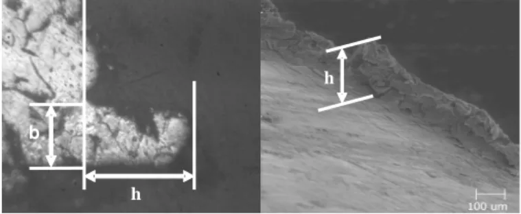
The burr can be characterized by their geometrical dimensions and two parameters are normally used: its thickness “b” and its height “h”, as illustrated in Fig. 1.
to the depth of cut, and for the other type of burrs the authors observed an increase in the burr height up to 5 mm with the increase of the depth of cut when they are formed by the main cutting edge. When they are formed by the secondary cutting edge, their heights were constant against the variation of the depth of cut, mainly when this parameter was over 0.5 mm.
Figure 1. Main parameters used to characterize a burr: its thickness “b” and its height “h” (Silva, J. D. et al., 2005).
Studies on burr formation and burr behavior comprise one active research area at the Machining Research and Teaching Laboratory (LEPU) of the School of Mechanical Engineering (FEMEC) of Federal University of Uberlândia (UFU). The first work was presented by Kaminise et al. (2001) and by Machado et. al. (2003) after studying burr formation processes in turning of AISI 1045 carbon steel. This was followed by the works developed by Da Silva (2004) and by Silva et al. (2005) when the burrs formed during face milling of engine blocks were studied. In this latter, the burrs were measured using metallographic techniques.
Following this research line the present work aims to optimize the cutting conditions in order to minimize the burr height in face milling of plastic injection mold steel. To measure their dimensions the burrs were reproduced with the aid of a mass used by the dentists to make prosthesis. This will be explained in details on the next item.
Nomenclature
B = burr thickness, mm Cr = chromium, chemical element doc = deph of cut, mm
fZ = feed per tooth, mm/z h = burr height, mm
Mo = molybdenum, chemical element Ni = nickel, chemical element Ra = roughness average, µm
Rt = the vertical distance between the highest pick and lowest
valley of the profile within the evaluation length, µm VBBmax= maximum flank wear, µm
Vc = cutting speed, m/min
Wt = the vertical hight between the highest and lowest point
of the profile in the wave range, µm
Experimental Procedure
Pre tests were carried out with the cemented carbides chosen to find out the limits in terms of cutting speed and feed rate in which the tool would work without breaking. Face milling tests were carried out in bars of AISI P20 steel used for plastic injection mold. The objective is to optimize the cutting speed, the feed per tooth and the depth of cut in order to minimize the burr height. The surface response technique was used after adopting a central composite design (CCD) resulting in 32 tests [16 tests (2k +2K + 2) + 1 replica] (Myers, 1976). The levels of the parameters used are shown in Tab. 1.
Table 1. Level of the parameters used in the tests.
Parameter levels
Cutting speed (m/min)
Feed per tooth (mm/tooth)
Depth of Cut (mm)
-1.28719 100 0.05 0.3
-1 125.54 0.0723 0.489
0 210 0.15 1.15
+1 295.46 0.228 1.81
+1.28719 320 0.25 2.0
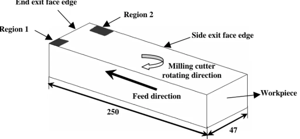
Two regions shown in Fig. 2 were chosen for reproduction of the workpiece edge in order to measure the burr heights. These regions were chosen because during pre-tests they were critical in terms of burr dimensions. Thus, when optimizing the cutting conditions for minimization of the burrs in these regions, the burrs in other parts of the workpiece were also reduced or even eliminated.
Table 2 shows the levels and the sequence of the tests. In each cutting condition the following steps were accomplished:
• Cutting operation – face milling of the workpiece surface in one pass, after introducing the cutting parameters (Vc, fz and doc) in the CNC machine center.
• Cleaning of the surface edge with a jet of compressed air for posterior molding for reproduction of the burr.
• Measurement of the burr generated in the two regions outlined in Fig. 2.
• Deburring with the aid of a file for starting the next test.
h
b
Figure 2. Identification of the regions where the burrs were reproduced for measuring their dimensions.
Table 2. Level of the parameters and sequence of the tests.
Test Number
Cutting speed
Feed per tooth
Depth of Cut
Test Number
Cutting speed
Feed per tooth
Depth of Cut
1 -1.00000 -1.00000 -1.00000 17 -1,00000 -1,00000 -1,00000
2 -1.00000 -1.00000 1.00000 18 -1,00000 -1,00000 1,00000
3 -1.00000 1.00000 -1.00000 19 -1.00000 1.00000 -1.00000
4 -1.00000 1.00000 1.00000 20 -1.00000 1.00000 1.00000
5 1.00000 -1.00000 -1.00000 21 1.00000 -1.00000 -1.00000
6 1.00000 -1.00000 1.00000 22 1.00000 -1.00000 1.00000
7 1.00000 1.00000 -1.00000 23 1.00000 1.00000 -1.00000
8 1.00000 1.00000 1.00000 24 1.00000 1.00000 1.00000
9 -1.28719 0.00000 0.00000 25 -1.28719 0.00000 0.00000
10 1.28719 0.00000 0.00000 26 1.28719 0.00000 0.00000
11 0.00000 -1.28719 0.00000 27 0.00000 -1.28719 0.00000
12 0.00000 1.28719 0.00000 28 0.00000 1.28719 0.00000
13 0.00000 0.00000 -1.28719 29 0.00000 0.00000 -1.28719
14 0.00000 0.00000 1.28719 30 0.00000 0.00000 1.28719
15 (C) 0.00000 0.00000 0.00000 31 (C) 0.00000 0.00000 0.00000
16 (C) 0.00000 0.00000 0.00000 32 (C) 0.00000 0.00000 0.00000
The value of “h” considered was the average of ten measurements taken on distinct points of the border on regions 1 and 2, respectively (Fig.2). These ten points were determined after dividing the sample length (Fig. 3) in ten equal parts, and cutting them according to Fig. 4. The amount of values considered (ten) for the average is justified by the considerable random variation of the burr height along the workpiece edge.
A mass proper for molding in dentistry with a base of polysulphide (Kerr mass) and with medium viscosity was melt in the regions 1 and 2 respectively with the aid of a small steel mold (Fig. 3). This technique allowed reproducing the morphological details of the burrs and the measurements of them.
Region 1
End exit face edge
f
25
f
250
47
Workpiece Side exit face edge
Region 2
Feed direction
The heights h were determined with the aid of an image analyzing system (Image Pro-Express). The system of reproduction of the burr avoids destroying the workpiece to take live samples for burr measurements. The mold is cut instead.
The workpiece was an AISI P20 steel used for injection mold of plastic produced by Villares Metals S/A of which own designation for them is VP20 steel. They are Cr-Ni-Mo alloyed steel obtained by vacuum degasification and are available in quenched and tempered condition with hardness of 30-34 HRC. Actual hardness of the workpiece used in this investigation is 32.4 HRC, with a standard deviation of 0.54.
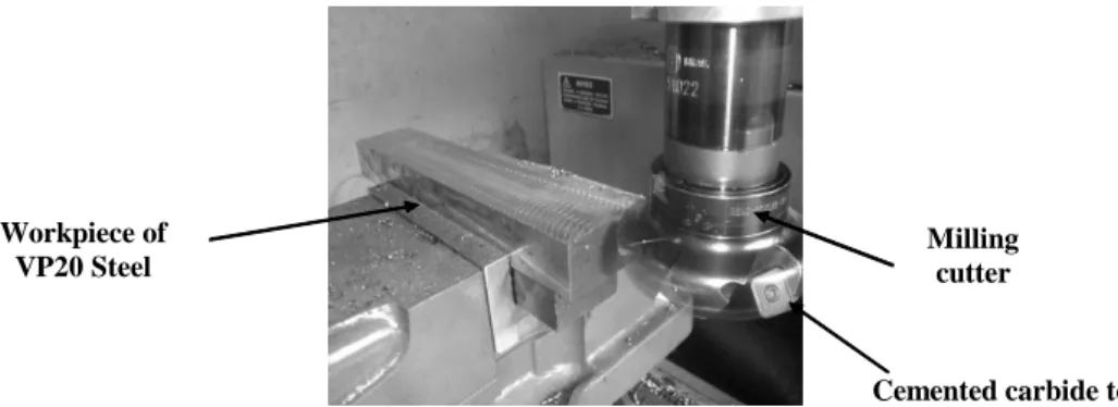
The machine tool was a CNC Milling Center Interact 4 manufactured by ROMI with 7.5 cv of power. A Sandvik face milling cutter R245063022 with 63 mm of diameter and capacity of 5 teeth was used. The cemented carbide tool inserts, also manufactured by Sandvik, were of the type R245-12 T3 M – class PM 4030 (covering ISO class P10 – 40 and M 10 to 25, according to the manufacturer’s catalogue). The tool tips were all fresh edges with no wear at all (VBBmáx = 0). Figure 5 shows the tooling and the workpiece set-ups.
Figure 5. Set-up of the workpiece and the milling cutter.
After the machining tests, individual models of the burr height of regions 1 and 2 against the cutting conditions were determined and represented by a Surface Response Technique. For this purpose, two techniques were used: the Statística 6.0 software and a coding developed by the authors in Matlab that uses the Multiple Polynomial Regression (MPR). The Statística 6.0 software besides developing the design of the experiments (CCD), it also generates the polynomial coefficients of the models. In this case, two models were generated for each region: the first one considering all the coefficients and the second one considering only the significant ones.
After determining all feasible surfaces that represent the behavior of the burr height in regions 1 and 2 against the cutting parameters, they were considered as the objective function of an optimization problem. For its solution, aiming the minimization of the burr height, two algorithms were used. The first one applies sequential methods using a toolbox of the Matlab (fminmax) and the
second one uses a random method namely Differential Evolution (Storn and Price, 1997) of which code was also developed in Matlab. After optimization new tests were carried out using the optimal results for model validation.
Results and Discussions
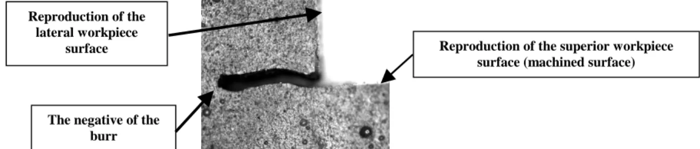
The method used for the burr height measurements was proven efficient and reproduces quite nicely the phenomenon. Figure 6 shows a cross section of a mold made with the polysulphide mass taken from region 1 of the workpiece after a test. This photo was taken within an optical microscopy. The image analyzer software is able to precisely determine the burr height, as illustrated in Fig. 7. Tab. 3 shows the average values of the burr heights found in each test at regions 1 and 2 of Fig.2.
Figure 3. Reproduction of the surface edges. Figure 4. Cutting of the burr mold.
Cemented carbide tool Workpiece of
VP20 Steel
Figure 6. An example of the reproduction of a burr formed at the exit border of the workpiece (region 1 of Fig. 2) in polysulphide based mass (magnification - 45X).
Figure 7. Example of a burr height measurement.
Table 3. Average height of the burrs “haverage” (µµµµm).
Replica 1 Replica 2
Region 1 Region 2 Region 1 Region 2
Tests
haverage
(µµµµm)
Standard Deviations
haverage
(µµµµm)
Standard Deviations
Tests
haverage
(µµµµm)
Standard Deviations
haverage
(µµµµm)
Standard Deviations
1 341.9 13.37 434.4 27.73 17 463.7 32.45 506.3 9.00
2 173.7 67.92 133.7 25.85 18 125.1 80.54 1468.7 221.43
3 563.2 41.84 516.8 16.86 19 465.3 49.23 484.6 47.86
4 1741.3 154.14 175.8 35.13 20 1720.9 429.76 1503.9 287.46
5 424.19 123.35 473.5 22.71 21 544.2 43.78 524.7 33.80
6 1649.9 156.86 213.9 25.49 22 1724.5 47.11 1580.9 63.54
7 442.4 45.77 437.4 57.79 23 645.3 203.84 489.7 21.00
8 1954.9 288.44 175.6 16.57 24 1713.8 43.04 1619.3 114.28
9 1010.8 38.86 947.3 112.70 25 1042.1 45.99 1148.8 53.91
10 1016.8 44.36 1055.3 26.92 26 1071.3 67.40 1039.1 47.53
11 1051.8 79.55 911.3 79.99 27 1162.5 35.02 1136.7 32.79
12 1215.2 98.82 1100.1 59.96 28 999.0 21.24 1070.9 22.33
13 331.9 136.36 269.8 28.16 29 301.9 30.24 345.8 27.36
14 1928.0 83.57 1805.5 90.60 30 1923.2 60.28 1865.4 56.84
15 1085.6 28.14 948.4 76.93 31 1089.9 58.67 1088.3 67.13
16 1015.7 21.16 1022.6 46.51 32 1077.5 51.16 1014.7 26.91
500 µµµµm
1698 µµµµm
Reproduction of the superior workpiece surface (machined surface) Reproduction of the
lateral workpiece surface
Pareto’s charts illustrated in Fig. 8 show the most significant cutting parameters for the burr height in the two regions considering a confidence interval of 95%. As can be observed, all the cutting parameters were significant for the burr height in region 1. Thus, it is expected that once the optimization procedure was undertaken for region 1, the burr height of region 2 will also be reduced. The results obtained by the Statistica 6.0 software demonstrated that the depth of cut affects directly the burr height of the two regions. Therefore it is hoped that optimizing the depth of cut for the region 1 the burr height in region 2 will also be reduced.
This behavior is confirmed by the results of tests with increasing depth of cut, where the burr height also increased proportionally. This is in accordance with results obtained by Kishimoto et al. (1981).
The Response Surfaces obtained using the three different techniques are shown in Tab. 4. Combination of the three Response Surfaces with the two methods of optimization allowed six strategies to be defined of which optimum results are shown in Tab. 5. The cutting parameters and the burr heights for each optimization strategy are presented.
Figure 8. “Pareto’s charts”: (a) Region 1; (b) Region 2.
Table 4. Response Surface obtained.
Response Surface* Origin of the Polynom
A 1166.8 + 199.0X(1) + 111.2X(2) + 481.8X(3) - 124.2X(1)
2 - 80.8X(2)2
- 72.3X(3)2 - 105.5X(1)X(2) + 200.9X(1)X(3) + 64.5X(2)X(3) = 0 MPR
B 1000.565 + 156.860X(1) + 167.915X(2) + 488.578X(3)
- 185.793X(1)X(2) + 191.268X(1)X(3) + 194.716X(2)X(3) = 0
Statistica 6.0 – with only the significant coefficients
C 1142.456 + 156.478X(1) + 167.533X(2) + 488.959X(3) - 185.254X(1)X(2) + 190.729X(1)X(3) + 194.177X(2)X(3) - 98.516X(1)2 - 55.152X(2)2 - 46.615X(3)2 = 0 Statistica 6.0 – all coefficients
* Where X(1) = Cutting speed; X(2) = feed per tooth and X(3) = depth of cut
Table 5. Optimization of the cutting parameters possible.
Optimization strategy
Response Surface used
Optimization algorithm used
VC
(m/min)
fz
(mm/z)
doc (mm)
Expected burr height
(µµµµm)
1 A fminimax 103.109 0.0549 0.3191 0
2 B fminimax 100 0.05 2.0 264.0572
3 C fminimax 100 0.05 0.3 94.9637
4 A DE 100 0.0859 0.3 75.0092
5 B DE 320 0.25 0.3 157.6503
6 C DE 320 0.25 0.3 346.3996
doc (L) fZ (L) fZ (L) by doc (L) Vc (L) by doc (L)
Vc (L) Vc (L) by fZ (L) Vc (Q) fZ (Q) doc (Q)
(a)
doc (L)
fZ (L) fZ (L) by doc (L) Vc (L) by doc (L)
Vc (L) Vc (L) by fZ (L) Vc (Q) fZ (Q) doc (Q)
New tests were carried out for each optimum cutting conditions and the average burr height found are shown in Tab.6. Strategies 5 and 6 obtained equal results for the cutting conditions. For strategy 2, the test was not possible to be done because the depth of cut was large and the cutting speed was reasonably low, causing tool breakage during machining. This result indicates that for future
works constrains for practical values of the cutting parameters should be added to the optimization problem.
Although the tests carried out considered optimum results only for the burr heights of region 1, the burr heights at region 2 were also analyzed and, as expected, the burr also reduced.
Table 6. Burr height obtained after optimization.
REGION 1 REGION 2
OPIMIZATION STRATEGY
haverage (µµµµm) Standard deviation
haverage
(µµµµm) Standard deviation
1 61.65 65.94 436.44 32.66
3 295.49 226.37 236.26 73.04
4 50.11 31.59 127.43 96.26
5 and 6 67.97 41.91 374.62 33.91
It can be seen that the optimization strategy number 4 stands out because it gave the smallest burr height in region 1 among all, and showed a reasonable small burr height at region 2, when compared with the results found experimentally in Tab. 3.
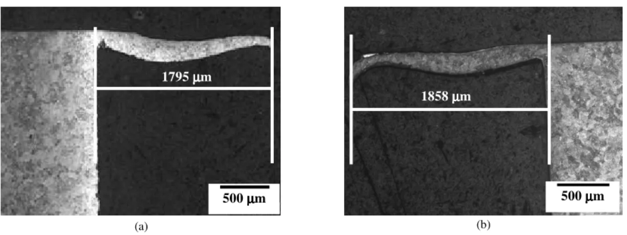
Figure 9 shows micrographs of the burrs formed at region 1 and 2 respectively, for the test number 14 that presented the biggest burr height among all. In this figure the burr dimensions are identified.
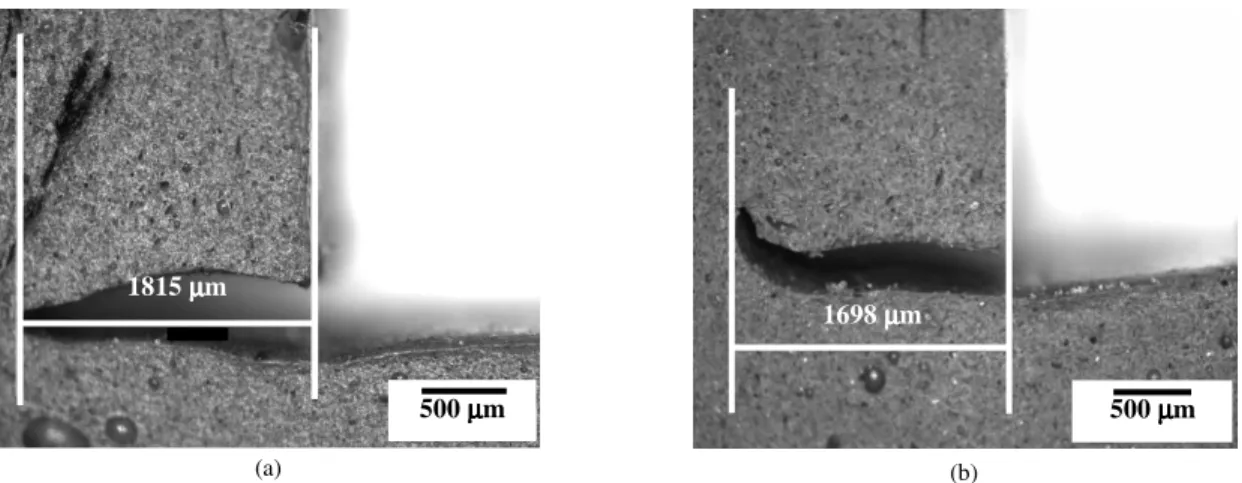
When these heights are compared to those presented in Fig 10, which were obtained by the technique that uses polysulphide based mass mold to reproduce the burr, they are quite similar, proving that this technique is accurate enough for burr studies. The small differences are attributed to variations of burr dimensions at different points of analysis.
Figure 9. Micrographs of the burrs formed during test 14 etched with Nital 4% and magnification of 50X: (a) Region 1; (b) Region 2. 500 µµµµm
1858 µµµµm
(b) 500 µµµµm
1795 µµµµm
Figure 10. Dimensions of the burr generated during test 14 were determined using the mold of polysulphide based mass (burr reproduction technique): (a) Region 1; (b) Region 2.
Higher magnifications of the burr root formed at region 1 of test 14 is shown in Fig. 11. It can be noticed that the burr root
suffers intense plastic deformation and this process may compromise the burr integrity.
Figure 11. (a) Burr root obtained at region 1 of test 14; (b) Detail shown in (a).
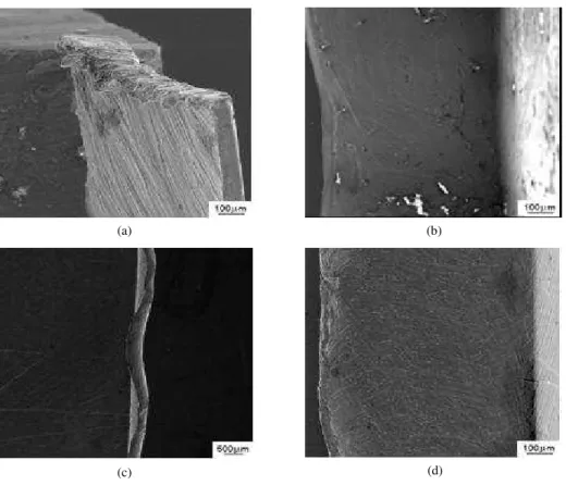
Figure 12 shows SEM photographs of the burrs formed during test 14. Details of the burrs at region 1 and 2 are clearly seen. The shapes of these burrs lead to a classification as rollover burr
according to Gillespie and Blotter (1976) at region 1, and as wave-type burr according to Lin (1999) at region 2.
500 µµµµm
1815 µµµµm
(a)
500 µµµµm
1698 µµµµm
(b)
Figure 12. SEM photos of the burrs formed during test 14: (a) Burr at region 1 - rollover burr; (b) Bottom view of the same burr; (c) Burr at region 2 – Wave-Type Burr; (d) Bottom view of the same burr.
Finally, Fig. 13a presents the bottom view of the burr formed at test 16 at the region 1 which is classified as a knife-type burr, and Fig. 13b presents the bottom view of the burr formed at region 2
which is classified as a saw-type burr according to Lin (1999). These photos were taken with a digital stereo microscopy.
Figure 13. (a) Bottom view of the burr formed during test 16 at region 1 (Mag. 20X); (b) Bottom view of the burr formed during test 16 at region 2 (Mag. 15X).
(a) (b)
(a) (b)
Conclusions
The following conclusions can be drawn from the present investigation.
The best results were calculated using the surface response obtained from the algorithm that uses the MPR – Multiple Polynomial Regression. It represents the best fit model for the burr height considering the cutting conditions. For the burrs at the two investigated regions the linear coefficients of the surfaces are more significant than the square coefficients.
The Differential Evolution Optimization technique was the most efficient process of minimization of the burr. It is a random algorithm and this methodology is strongly indicated for optimization problem that contains several local minimums.
The tests carried out with the cutting conditions indicated by strategy 4 (see Tabs. 5 and 6) produced a burr height with an error of - 33.2% from the minimized burr indicted by the optimization with the smallest standard deviation among all strategies.
With the cutting condition optimized for the burr height of region 1, the dimensions of the burr at region 2 were also reduced considerably. The high standard deviation for the region 2 indicates that the burrs at this face present high level of dimensional variation. It is worth mentioning that in some points of this region there was no burr at all, when using the optimized cutting conditions obtained by the strategy 4.
Although this refers to an initial study, the results obtained joining the DOE – Design of Experiments, Surface Response and optimization techniques are very interesting and encouraging. Tests carried out using the indicated optimized cutting conditions proved considerable reduction of the burr height during face milling of VP 20 steel. All this indicates that further research in this line are very promising.
Acknowledgements
The authors are grateful to Villares Metals SA for providing the work material and the SEM photos of the burrs, and to CNPq, CAPES, FAPEMIG and IFM for financial support.
References
Da Silva, L.C., 2004, “Study of the burr in face milling of engine blocks of grey cast iron using ceramic and PCBN tool inserts” (In Portuguese), Master dissertation, Programa de Pós-graduação em Engenharia Mecânica, FEMEC, UFU, Uberlândia, MG, 179 p.
Gillespie, L.K. and Blotter, P.T., 1976, “The formation and properties of
machining burrs”, Transactions of the ASME, pp. 66-74.
Kaminise, A.K., Da Silva, M.B. and Ariza, R.G., 2001, “Study on burr
formation in turning AISI 1045”, Proceedings of 16th COBEM Brazilian
Congress of Mechanical Engineering, paper code 0147, Uberlândia, MG, Brazil.
Kishimoto, W., Miyake, T., Yamamoto, A., Yamanaka, K. and Tacano,
K., 1981, “Study of burr formation in face milling”, Bull. Japan Soc. of Prec.
Eng., Vol. 15, No 1, pp. 51-52.
Ko, S.L. and Dornfeld, D.A., 1991, “A study on burr formation
mechanism”, Journal of Engineering Materials and Technology, Vol.113,
pp.75-87.
Ko, S.L. and Dornfeld. D.A., 1996a, “Analysis of fracture in burr
formation at the exit stage of metal cutting”, Journal of Materials Processing
Technology, Vol. 58, pp. 189-200.
Ko, S.L. and Dornfeld. D.A., 1996b, “Burr formation and fracture in
oblique cutting”, Journal of Materials Processing Technology, Vol. 63, pp.
24-36.
Lin, T.R, 1999, “Experimental study of burr formation and tool chipping
in the face milling of stainless steel”, Journal of Materials Processing
Technology, Vol. 108, pp. 12-20.
Machado, A.R., Kaminise, A.K., Da Silva, M.B. and Ariza, R.G.,
”Study on burr formation in turning”, Proceedings of 17th COBEM Brazilian
Congress of Mechanical Engineering, São Paulo, SP, Brazil.
Myers, R.H., 1976, “Response Surface Methodology”, 1st Edition, 246 p.
Nakayama, K. and Arai, M., 1987, “Burr formation in metal cutting”,
Annals of the CIRP, Vol. 36, pp. 33-36.
Olvera, O. and Barrow, G., 1995, “An experimental study on burr
formation in square shoulder face milling”, Intl. J. Machine Tools and
Manufacture, Vol. 36, No. 9, pp. 1005-1020.
Pekelharing, A.J., 1978, “The exit failure uninterrupted cutting”, Annals
of the CIRP, Vol. 27, No. 1, pp.5-10.
Silva, J.D., Da Silva, L.C., Ariza, R.G., Souza, Jr. A.M. and Machado, A.R., 2005, “Characterization of burr formed on engine blocks using
metalographic techniques”, Proceedings of 18th COBEM Brazilian Congress
of Mechanical Engineering, Ouro Preto, MG, Brazil.
Storn, R. and Price, K., 1997, “Differential evolution -a simple and
efficient heuristic for global optimization over continuous spaces”, Journal