Article
J. Braz. Chem. Soc., Vol. 23, No. 9, 1669-1679, 2012. Printed in Brazil - ©2012 Sociedade Brasileira de Química 0103 - 5053 $6.00+0.00
A
*e-mail: [email protected]
Evaluation of Trace Metal Levels in Surface Sediments of the Sergipe River
Hydrographic Basin, Northeast Brazil
Aldair F. Silva,a George R. S. Lima,a Jeferson C. Alves,a Samir H. Santos,a Carlos A. B. Garcia,a
J. Patrocinio H. Alves,a,b Rennan G. O. Araujoa and Elisangela A. Passos*,a
aDepartamento de Química, Universidade Federal de Sergipe, 49100-000 São Cristóvão-SE, Brazil
bInstituto Tecnológico e de Pesquisa do Estado de Sergipe, 49020-380 Aracaju-SE, Brazil
As distribuições de Co, Cr, Cu, Mn, Ni, Pb, Fe e Al foram investigadas em sedimentos superficiais coletados em 19 sítios da Bacia Hidrográfica do Rio Sergipe, Nordeste do Brasil. Foi definida uma base geoquímica para a região (RGB) usando o ferro como elemento de referência. Fatores de enriquecimento (EF) e índice de geoacumulação (Igeo) foram empregados para determinar a contribuição por origem antropogênica. Valores de EF mostraram que os sedimentos dos sítios 1, 5 e 13 podem ser considerados contaminados por Pb, Cr e Cu, respectivamente. Valores de Igeo mostraram que o sítio 13 pode ser considerado contaminado. Há uma grande predominância nos sedimentos de metais de origem natural. A possível toxicidade foi avaliada comparando com os valores PEC-TEC dos guias de qualidade de sedimentos (SQG). Análise de componentes principais (PCA) separou claramente os pontos em dois grupos e a análise de agrupamento hierárquico (HCA) confirmou as interpretações feitas pela PCA.
The distributions of Co, Cr, Cu, Mn, Ni, Pb, Fe and Al were investigated in surface sediments collected at 19 sites in the Sergipe River Hydrographic Basin of Northeast Brazil. A regional geochemical baseline (RGB) was defined using iron as a reference element. Enrichment factors (EF) and geoaccumulation indices (Igeo) were used to determine the extent of anthropogenic metal pollution. EF values showed that sediments from sites 1, 5 and 13 could be considered contaminated by Pb, Cr and Cu, respectively. Igeo values showed that only site 13 could be considered contaminated. For other sites, results indicated that naturally occurring metals predominated in the sediments. Possible toxicity related to these metals was examined using the comparing sediment chemical data with sediment quality guidelines (SQG) PEC-TEC values. Principal component analysis (PCA) clearly separated the sites into two groups and hierarchical cluster analysis (HCA) confirmed the interpretations made from the PCA results.
Keywords: sediment, trace metals, Sergipe River, toxicity, multivariate analysis
Introduction
Metal pollutants have received considerable attention due to their persistence, biogeochemical recycling, and environmental risk.1 Sediments act as a reservoir for metals
introduced into the aquatic environment as a result of natural geochemical processes (such as weathering and erosion of geological formations) and anthropogenic activities (such as urbanization, industrialization, deforestation, land erosion and agricultural practices).2,3 Metals can be
remobilized and released from sediment into the overlying water column during chemical and biological processes.4,5
High metal concentrations in sediment do not automatically imply that contamination has occurred, but may simply reflect the natural mineralogical composition of the parent geological material, and the grain size and organic matter content of the host sediment.4,5 Many
studies of metal accumulation in the aquatic environment have focused on the establishment of geochemical baselines for evaluation of the magnitudes of natural and/ or anthropogenic metal inputs.2 Knowledge of background
metal concentrations, and the natural variability, is therefore necessary before assessments of anthropogenic impacts can be made.6 Various normalization procedures have been
Two procedures can be used to normalize metal concentrations: granulometric and geochemical normalizations.4 Granulometric normalization involves the
isolation of a defined grain size fraction by sieving, with the aim of reducing the dilution effects of non-metal-bearing minerals in coarse grained sediment.9,10 Geochemical
normalization is based on a procedure that involves mathematical correlations between metal concentrations and the concentrations of a reference element, such as Al, Fe, Li, or Sc. These reference elements are tracers for natural metal-binding phases, and are ideally not influenced by anthropogenic inputs.6,11-13 Chemical normalization has
the following advantages: (i) a single analytical procedure can be used to determine all necessary elements, including the pollutants and those used for normalization; (ii) minimal manipulation of the sample minimizes contamination; (iii) use of the chosen element (or elements) can normalize both grain size and compositional variability.14
It is accepted that determination of the total concentrations of metals in sediments is not sufficient to predict the capacity for mobilization of these elements.15-17 The environmental
behavior of trace metals is critically dependent on their chemical form, which influences mobility, bioavailability and toxicity to organisms. Consequently, there is considerable interest in understanding the associations of these elements with the solid phase.18,19
The sediment quality guidelines (SQG) system, developed by North American agencies has been adopted as an informal tool to evaluate sediment chemical data in relation to possible adverse effects on aquatic biota.8 The
consensus-based sediment quality guidelines for fresh waters have been established for 28 chemicals (metals, polycyclic aromatic hydrocarbons, polychlorinated biphenyls and pesticides) and for each contaminant provide two concentrations associated with adverse effects in aquatic organisms.20 The threshold effect concentration
(TEC) is that below which no adverse effects should occur, and the probable effect concentration (PEC) is that above which adverse effects may occur frequently.8,20
There has been no systematic evaluation of the metals present in the sediments of the Sergipe River Hydrographic Basin in Northeast Brazil, although a limited number of previous studies have investigated the water and sediment quality of individual rivers and estuarine regions of the basin.3,8,15,16,21 The present work therefore describes a
geochemical evaluation of trace metals in surface sediments of this river basin. Sediment samples were analyzed by inductively coupled plasma optical emission spectrometry (ICP OES), in order to define a regional geochemical baseline, to identify impacted areas and assess the extent of sediment contamination, and to distinguish natural and
anthropogenic inputs. Calculations were made of metal enrichment factors (EF) and geoaccumulation indices (Igeo).
Possible toxicity was evaluated for each metal, based on consensus-based SQG reference data. Potential factors controlling the distribution and mobility of metals in the sediments were also investigated. Statistical analyses (using PCA and HCA) were conducted in order to identify common origins and/or behaviors of the contaminants.
Experimental
Study area
The Sergipe River Hydrographic Basin is located in the State of Sergipe (population 1.01 million), in the Northeast of Brazil, between latitudes 10°21’S and 10°55’S, and longitudes 37°11’W and 37°41’W. It has an area of 3673 km2 and drains approximately 16.7% of
the State. The climate can be characterized as tropical, with an annual mean temperature of 25 °C and an average annual rainfall of 1333 mm.22 The main tributaries in the
basin are the Rivers Sovacão, Lages, Campanha, Jacoca, Vermelho, Jacarecica, Pitanga, Poxim, Salgado, Cágado, Ganhamoroba, Parnamirim and Pomonga.22
Since the 1990s, there has been rapid expansion of aquaculture, industry, and agriculture in the region, with simultaneous development in the areas of civil construction, transportation, and tourism. These dramatic changes have adversely affected water quality in the basin.21 The main
sources of trace metal contamination are municipal and industrial wastewaters, agricultural runoff, and emissions from metallurgical industries.15,23
Sample collection and pretreatment
Sediment samples were collected in December 2010, at nineteen locations including industrial, residential, commercial and rural sites, in the Sergipe River Hydrographic Basin (Figure S1, in Supplementary Information), using a core sampler composed of cellulose acetate butyrate. The undisturbed upper 5 cm of the sediment was sampled, and then placed in acid-rinsed polypropylene vessels using a plastic spatula. Three samples were taken at each location. The sediments were oven-dried (50 °C, 12 h), homogenized in a porcelain mortar, sieved (< 2 mm), and stored in plastic containers until the analyses were performed.3
Reagents
system. All glass and plastic utensils were washed with 10% (v/v) nitric acid for 48 h, and rinsed with ultrapure water prior to use. Stock metal standard solutions (1000 mg L−1)
were prepared from standard vials (Tritisol, Merck) containing 1.000 ± 0.002 g of metal in 2% (v/v) nitric acid. Calibration standards of each metal were obtained by suitable dilutions of the stock solutions. Three certified reference materials, LKSD-1 CCNRP (Canada lake sediment), NCS DC 75304 (China river sediment) and NCS DC 78301 (China marine sediment) were analyzed for quality control purposes.
Total metals extraction procedure
The metals were extracted by digesting portions (ca. 0.5 g) of the samples in closed Teflon vessels with 2 mL of HNO3, 1 mL of HCl and 4 mL of HF, at 140 oC for 2 h.
After cooling, the vessels were opened and heated at 210 oC
to complete dryness. The residue was dissolved in 10 mL of 0.5 mol L-1 HCl, and the final volume was made up to
50 mL.16 The solutions were stored in polyethylene flasks
for later determination of metals using ICP OES.
Calculation of the limit of detection (LOD) for each metal was based on the expression 3s/b, where s is the standard deviation of the blank, and b is the slope of the calibration plot.24 Ten extraction procedure blanks were
analyzed, and LOD values took into account the use of 1 g portions of sample in extractions, together with any necessary dilutions. Correlation coefficients (r) of the calibration curves were better than 0.998, for all elements studied. The results showed that there was no significant analytical contamination, and that LOD values varied from 0.04 (Cr and Mn) to 0.32 µg g−1 (Al). These limits
of detection are acceptable for general environmental analyses, and are comparable to those obtained in previous work using similar materials.16,25-27
The efficiency of the extraction method was determined by analysis of four replicates of certified reference material (CRM), for river sediment (NCS DC 75304/China) and marine sediment (NCS DC 78301/China). The results showed that recoveries of the metals from the CRMs were in the range 81-103%. These values indicate that the efficiency of the method was satisfactory, given the complex nature of the sediment matrix. Similar values have been reported in the literature.8,21,25,28
Partial metals extraction procedure
Partial metal concentrations were determined using US EPA Method 200.8. Samples (ca. 1 g) were treated in closed Teflon vessels using 4 mL of (1+1) HNO3 solution
and 10 mL of (1+5) HCl solution. The mixtures were heated at 95 oC for 30 min. Following extraction, the samples
were filtered using quantitative filter paper, transferred to 50 mL volumetric flasks, and the volumes were made up using ultra-pure water.16 The solutions were stored in
polyethylene flasks for later determination of metals using ICP OES.
Ten blank solutions were prepared in the same way as samples during the digestion procedure, and for quality control purposes a lake sediment reference material (LKSD-1 CCNRP/Canada) was analyzed alongside the samples. LOD values (in µg g−1) varied from 0.001 (Cd)
to 0.080 (Pb). Recoveries of the trace metals were in the range 97-103%.
Organic carbon determination
The carbon contents of the samples were determined using an elemental analyzer with a combustion temperature of 900 oC. The organic carbon (C
org) content was calculated
by the difference in the amount of carbon determined before and after calcination of the samples at 550 oC for 1 h.3 For
analytical quality control, each set of sample analyses was accompanied by three replicate analyses of lake sediment reference material (LKSD-1 CCNRP/Canada), for which the mean recovery was 98.4 ± 0.7%.
Instrumentation
Sediment extractions were performed using PTFE vessels and a digester block (Techal TE007A). The carbon contents of the samples were measured using an NCHS-O elemental analyzer (Flash ES 1112).
An inductively coupled plasma optical emission spectrometer (ICP OES) with an axial view configuration (VISTA PRO, Varian, Mulgrave, Australia) was used for the determination of aluminium, cobalt, chromium, copper, iron, manganese, nickel, lead and zinc. The ICP OES system was equipped with a solid-state CCD that enabled simultaneous measurements to be made in the range 167-785 nm. The instrumental parameters were as follows: 40 MHz radio frequency; 1100 W applied power; 15.0 L min−1 plasma gas flow rate; 1.5 L min−1 auxiliary gas
flow rate; 0.8 mL min−1 nebulizer gas flow rate; 0.8 mL min−1
emission line, and “II” indicates the ionic emission line. In most cases, the wavelengths were selected according to the most prominent line; secondary lines were used as an alternative to avoid possible interferences. All analyses were performed in triplicate.
Statistical analysis
Principal component analysis (PCA), hierarchical cluster analysis (HCA) and correlation coefficient calculations were performed using the program Statistica for Windows v. 6.0 (StatSoft Inc., USA). One-way analysis of variance (ANOVA) and Tukey’s multiple comparison test were employed (using Origin v. 7.0) to test for significant differences (p ≤ 0.05) in metal concentrations among the sites.
Results and Discussion
Metal and organic carbon distributions
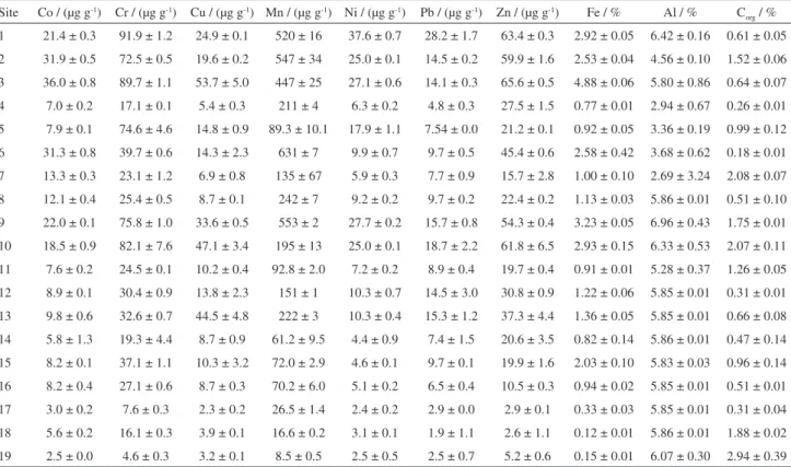
The metal and organic carbon contents of the samples are presented in Table 1. The ranges of concentrations found were (in µg g-1) 2.5-35.9 (Co); 4.6-91.9 (Cr);
2.3-53.7 (Cu); 2.4-37.5 (Ni); 1.9-28.2 (Pb); 2.6-65.6 (Zn)
and (in %) 0.1-4.9 (Fe); 2.7-6.9 (Al). The highest values of all elements were obtained for sites 1-3. This could be due to either natural variability between the sediments, or to anthropogenic contamination.5,29,30 Organic carbon
(Corg) contents varied between 0.2 and 2.9%, with highest
values for sites 7, 10 and 19, indicating an anthropogenic contribution.22 The main sources of organic matter are
municipal and industrial wastewaters, and agricultural runoff.15
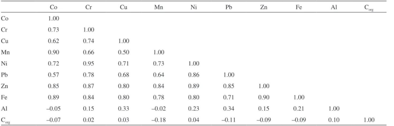
Correlation analysis was used to identify potential factors controlling the distribution and mobility of metals in the sediments. The Spearman correlation matrix obtained is provided in Table 2. The linear regression analysis can provide information about the similarity of natural and anthropogenic sources, as well as the environmental behavior of metals. Significance was indicated by values of the correlation coefficient greater than 0.60 (using a confidence level of 95%).
Strong correlations were observed between most of the trace metals and iron (r > 0.7) and manganese (r > 0.6), with the exception of Cu (r = 0.5). However, weak correlations were observed with aluminum (r < 0.4) (Table 2). The strong correlations between manganese and iron, and between iron and the other metals, showed that iron and manganese were the main inorganic carriers that controlled
Table 1. Metal concentrations and organic carbon (Corg) contents in the surface sediments of three regions of the Sergipe River Basin (n = 3, mean ± standard deviation)
Site Co / (µg g-1) Cr / (µg g-1) Cu / (µg g-1) Mn / (µg g-1) Ni / (µg g-1) Pb / (µg g-1) Zn / (µg g-1) Fe / % Al / % C org / %
1 21.4 ± 0.3 91.9 ± 1.2 24.9 ± 0.1 520 ± 16 37.6 ± 0.7 28.2 ± 1.7 63.4 ± 0.3 2.92 ± 0.05 6.42 ± 0.16 0.61 ± 0.05
2 31.9 ± 0.5 72.5 ± 0.5 19.6 ± 0.2 547 ± 34 25.0 ± 0.1 14.5 ± 0.2 59.9 ± 1.6 2.53 ± 0.04 4.56 ± 0.10 1.52 ± 0.06
3 36.0 ± 0.8 89.7 ± 1.1 53.7 ± 5.0 447 ± 25 27.1 ± 0.6 14.1 ± 0.3 65.6 ± 0.5 4.88 ± 0.06 5.80 ± 0.86 0.64 ± 0.07
4 7.0 ± 0.2 17.1 ± 0.1 5.4 ± 0.3 211 ± 4 6.3 ± 0.2 4.8 ± 0.3 27.5 ± 1.5 0.77 ± 0.01 2.94 ± 0.67 0.26 ± 0.01
5 7.9 ± 0.1 74.6 ± 4.6 14.8 ± 0.9 89.3 ± 10.1 17.9 ± 1.1 7.54 ± 0.0 21.2 ± 0.1 0.92 ± 0.05 3.36 ± 0.19 0.99 ± 0.12
6 31.3 ± 0.8 39.7 ± 0.6 14.3 ± 2.3 631 ± 7 9.9 ± 0.7 9.7 ± 0.5 45.4 ± 0.6 2.58 ± 0.42 3.68 ± 0.62 0.18 ± 0.01
7 13.3 ± 0.3 23.1 ± 1.2 6.9 ± 0.8 135 ± 67 5.9 ± 0.3 7.7 ± 0.9 15.7 ± 2.8 1.00 ± 0.10 2.69 ± 3.24 2.08 ± 0.07
8 12.1 ± 0.4 25.4 ± 0.5 8.7 ± 0.1 242 ± 7 9.2 ± 0.2 9.7 ± 0.2 22.4 ± 0.2 1.13 ± 0.03 5.86 ± 0.01 0.51 ± 0.10
9 22.0 ± 0.1 75.8 ± 1.0 33.6 ± 0.5 553 ± 2 27.7 ± 0.2 15.7 ± 0.8 54.3 ± 0.4 3.23 ± 0.05 6.96 ± 0.43 1.75 ± 0.01
10 18.5 ± 0.9 82.1 ± 7.6 47.1 ± 3.4 195 ± 13 25.0 ± 0.1 18.7 ± 2.2 61.8 ± 6.5 2.93 ± 0.15 6.33 ± 0.53 2.07 ± 0.11
11 7.6 ± 0.2 24.5 ± 0.1 10.2 ± 0.4 92.8 ± 2.0 7.2 ± 0.2 8.9 ± 0.4 19.7 ± 0.4 0.91 ± 0.01 5.28 ± 0.37 1.26 ± 0.05
12 8.9 ± 0.1 30.4 ± 0.9 13.8 ± 2.3 151 ± 1 10.3 ± 0.7 14.5 ± 3.0 30.8 ± 0.9 1.22 ± 0.06 5.85 ± 0.01 0.31 ± 0.01
13 9.8 ± 0.6 32.6 ± 0.7 44.5 ± 4.8 222 ± 3 10.3 ± 0.4 15.3 ± 1.2 37.3 ± 4.4 1.36 ± 0.05 5.85 ± 0.01 0.66 ± 0.08
14 5.8 ± 1.3 19.3 ± 4.4 8.7 ± 0.9 61.2 ± 9.5 4.4 ± 0.9 7.4 ± 1.5 20.6 ± 3.5 0.82 ± 0.14 5.86 ± 0.01 0.47 ± 0.14
15 8.2 ± 0.1 37.1 ± 1.1 10.3 ± 3.2 72.0 ± 2.9 4.6 ± 0.1 9.7 ± 0.1 19.9 ± 1.6 2.03 ± 0.10 5.83 ± 0.03 0.96 ± 0.14
16 8.2 ± 0.4 27.1 ± 0.6 8.7 ± 0.3 70.2 ± 6.0 5.1 ± 0.2 6.5 ± 0.4 10.5 ± 0.3 0.94 ± 0.02 5.85 ± 0.01 0.51 ± 0.01
17 3.0 ± 0.2 7.6 ± 0.3 2.3 ± 0.2 26.5 ± 1.4 2.4 ± 0.2 2.9 ± 0.0 2.9 ± 0.1 0.33 ± 0.03 5.85 ± 0.01 0.31 ± 0.04
18 5.6 ± 0.2 16.1 ± 0.3 3.9 ± 0.1 16.6 ± 0.2 3.1 ± 0.1 1.9 ± 1.1 2.6 ± 1.1 0.12 ± 0.01 5.86 ± 0.01 1.88 ± 0.02
the distribution of metals in these sediments. According to Sabadini-Santos et al.,2 the rivers of Northeast Brazil are the
main source of smectite and illite particles coated with iron oxyhydroxides found in the estuarine and near-shore coastal sediments of the region. A possible explanation for the relatively low correlation between Al and the other metals is natural variability of metal concentrations between sediments of the Sergipe River Basin. Iron has also been successfully used as a normalizer in other studies.2,5,6,9,31
The trace metals showed no correlation with Corg
(r < 0.10), indicative of no, or weak, association between these elements and organic matter in the sediments. This is in agreement with the finding that, in non-marine sediments, Corg is a weaker carrier than clays and metal oxides.8,32
There were significant correlations (0.62 < r < 0.95) between the different trace metals (Table 2), indicative of a natural origin and/or similar contamination sources of the metals. The correlation coefficients revealed that Fe was the most suitable conservative element for metal normalization purposes.
Geochemical normalization
In order to determine the extent of contamination of the sediments, trace metal concentrations were normalized relative to iron. Various reference elements have previously been used for this purpose, notably iron,2,5,32 aluminium,8,33,34
lithium8,13,29 and scandium.1,35,36
Geochemical normalization uses data obtained for uncontaminated sediments of a given region to calculate the linear regression between concentrations of the metal of interest and those of the reference element, and then tests the metal/reference ratios obtained for other (possibly contaminated) sites.13 The relationships between trace
metals and reference elements can be used to indicate the range of naturally occurring concentrations of trace
metals.5,29,37 The regressions between the metals and the
normalizer (reference element) are performed following removal of outlier values, and delineation of a 95% prediction interval. The data points obtained for a possibly contaminated area are then projected onto the resulting graph. All points lying within the 95% prediction intervals correspond to samples that can be characterized as natural sediments, while points located above this region may indicate sediment contamination.9,11,13
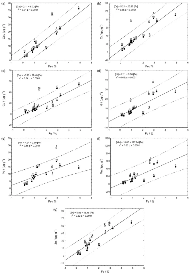
The linear regression results, with values of r2 and p,
as well as the 95% prediction intervals, are illustrated in Figure 1. The upper 95% prediction interval was used as the cutoff to identify metal enrichment in the sediments.
Mn and Zn (Figures 1f and 1g) showed similar distribution patterns, with all sites lying within the 95% prediction limits. The concentrations of Co, Cr, Cu, Ni and Pb showed enrichment at one or more sampling sites (Figures 1a-e), indicating possible contamination. Ni and Pb (Figures 1d and 1e) showed concentrations much higher than the 95% prediction limits at site 1, indicating strong enrichment of the metals in the sediment. Cobalt showed enrichment at sites 2 and 6 (Figure 1a), and there was possible anthropogenic influence for Cr (Figure 1b) at site 5. These sites were located in regions where there is intense agricultural activity.22 Copper was enriched
at site 13 (Figure 1c), located in the densely populated region.22 Hence, metal concentrations in the sediments
analyzed could be considered to be due to natural origins, except at sites 1, 2, 5, 6 and 13, and the regression lines obtained could be used to define the regional geochemical baseline (RGB).
The data using in the geochemical normalization were obtained by extraction using HF, HNO3 and HCl
to determine the total concentrations of metals. The total sediment concentration of a metal does not provide information concerning its mobility, availability or toxicity.
Table 2. Spearman’s correlation matrix for surface sediments (95% confidence limits, n = 19, p < 0.05)
Co Cr Cu Mn Ni Pb Zn Fe Al Corg
Co 1.00
Cr 0.73 1.00
Cu 0.62 0.74 1.00
Mn 0.90 0.66 0.50 1.00
Ni 0.72 0.95 0.71 0.73 1.00
Pb 0.57 0.78 0.68 0.64 0.86 1.00
Zn 0.85 0.87 0.80 0.84 0.89 0.85 1.00
Fe 0.89 0.84 0.80 0.78 0.80 0.71 0.90 1.00
Al –0.05 0.15 0.33 –0.02 0.23 0.34 0.15 0.21 1.00
Toxicity is dependent on the amount of metal available for bioaccumulation (accumulation by organisms), and it depends on those sediment properties that affect its bioavailability. Hence, it is possible for sediment to be metal-contaminated (to have a metal content higher than the natural background), but not manifest any toxic effects, depending on the geochemical processes that control the availability of the metal in the sediment.
Enrichment factors (EF)
For better estimation of anthropogenic inputs, enrichment factors (EF) were calculated for each metal, as described by Aloupi and Angelidis,13 using the expression
([metal]/[Fe])sample/([metal]/[Fe])background, where
([metal]/[Fe])sample is the metal to Fe ratio in a sample, and
([metal]/[Fe])background is the natural background value of
the metal to Fe ratio. For any given Fe concentration, the metal concentration on the linear regression line was used as the background value, and the concentration lying on the upper 95% prediction limit was used as a comparison value (CV). Due to natural mineralogical differences between the sediments and analytical uncertainty, only sediments with an EF greater than 2.0 were considered to be enriched.38
Compared to other methods based on the use of global backgrounds, such as average shale values39 or average
crustal values,40 an advantage of the RGB technique is that
it takes into account the natural geochemical variability related to different settings and sediment characteristics.4
According to Mil-Homens et al.,41 the use of global
background data can result in erroneous interpretation of EF values, and underestimation of metal enrichment.
Table 3 shows calculated sediment enrichment factors for Co, Cr, Cu, Ni and Pb, together with comparison values. The EF values indicate that the most contaminated sediments were those from sites 1, 5 and 13, where there was substantial anthropogenic activity. Relatively strong enrichment of Cu (EF > 3) was found for site 13, located in an area of intensive ship traffic. According to Idris,17
enrichment by Cu is often related to ship maintenance
and the corrosion of metallic materials. The anti-fouling paint used on the hulls of ships is one of the major sources of pollution by Cu in the aquatic environment.42,43 There
was an enrichment of Cr at site 5 (EF < 3), which could be due to industrial activities. Silva et al.44 found a high
concentration of Cr associated with effluents from sugar, leather, and paper factories in the Mogi Guaçu River Basin of Southeast Brazil. Moderate Pb enrichment was only observed for site 1 (EF = 2.08), which could be due to inputs of agricultural effluents. Gimenon-Garcia et al.45
found that Pb was present as an impurity in fertilizers and pesticides applied to agricultural soils.
Geoaccumulation index (Igeo)
The geoaccumulation index (Igeo), first described by
Müller,46 was used here as a second criterion to identify
contaminated sediments (Table 4). Igeo is defined by the
expression: log2 [Cn/1.5Bn], where Cn is the measured
concentration and Bn is the geochemical background
concentration of the metal “n”. The factor 1.5 is a constant that helps take account of lithological variability. The metal concentration on the regression line was used as the background value, as reported in previous studies.1,8,47 I
geo
can then be used as a reference to estimate the extent of metal pollution, in a similar way as the enrichment factor.48
The index is based on a qualitative pollution intensity scale, whereby sediments can be classified as unpolluted
Table 3. Enrichment factors (EF) and comparison values (CV) for surface sediments from the Sergipe River Basin
Site Co Cr Cu Ni Pb
EF CV EF CV EF CV EF CV EF CV
1 0.98 1.41 1.39 1.39 0.84 1.48 1.91 1.58 2.08a 1.57
2 1.57 1.52 1.24 1.43 0.77 1.56 1.44 1.65 1.15 1.58
5 0.95 2.04 2.63a 2.22 1.64 2.54 2.21 2.33 1.00 2.00
6 1.58 1.45 0.67 1.42 0.56 1.57 0.56 1.64 0.76 1.59
13 0.86 1.76 0.97 1.74 3.45a 2.14 0.93 1.93 1.70 1.82
aEnrichment.
Table 4. Geoaccumulation index (Igeo) values for surface sediments from the Sergipe River Basin
Site Co Cr Cu Ni Pb
1 −0.62 −0.11 −0.84 0.47 0.35
2 0.06 −0.27 −0.96 −0.38 −0.06
5 −0.65 0.81 0.13 −0.58 0.56
6 0.08 −1.15 −1.43 −0.97 −1.42
13 −0.80 −0.63 1.20a 0.18 −0.69
(Igeo≤ 0), unpolluted to moderately polluted (0 ≤ Igeo≤ 1),
moderately polluted (1 < Igeo≤ 2), moderately to highly
polluted (2 < Igeo≤ 3), highly polluted (3 < Igeo≤ 4), highly
to extremely polluted (4 < Igeo≤ 5), and extremely polluted
(Igeo > 5).46
The sediments from sites 1, 2, 5, and 6 were classified as unpolluted with respect to the trace metals Co, Cr, Cu, Ni, and Pb (Table 4). Sediment from site 13 (near shipping activities) was in the unpolluted to moderately polluted category, with respect to Co, Cr, Ni and Pb, and in the moderately polluted category, with respect to Cu. The results obtained using both procedures (EF and Igeo)
therefore showed that only site 13 could be considered to be contaminated with Cu.
Sediment toxicity: TEC-PEC predictions
The TEC and PEC concentrations presented in the consensus-based sediment quality guidelines (SQG), developed by MacDonald et al.,20 have been adopted as
an informal tool to evaluate sediment chemical data in relation to possible adverse effects on aquatic biota. TEC and PEC values indicate concentrations at which toxicity could start to be observed, and above which adverse effects might occur, respectively.8,20 The SQG criteria were derived
and validated using data only for fresh water and marine ecosystems of the USA, but despite this limitation have been used to interpret data for sediments from various global regions.3,8,20,49-51
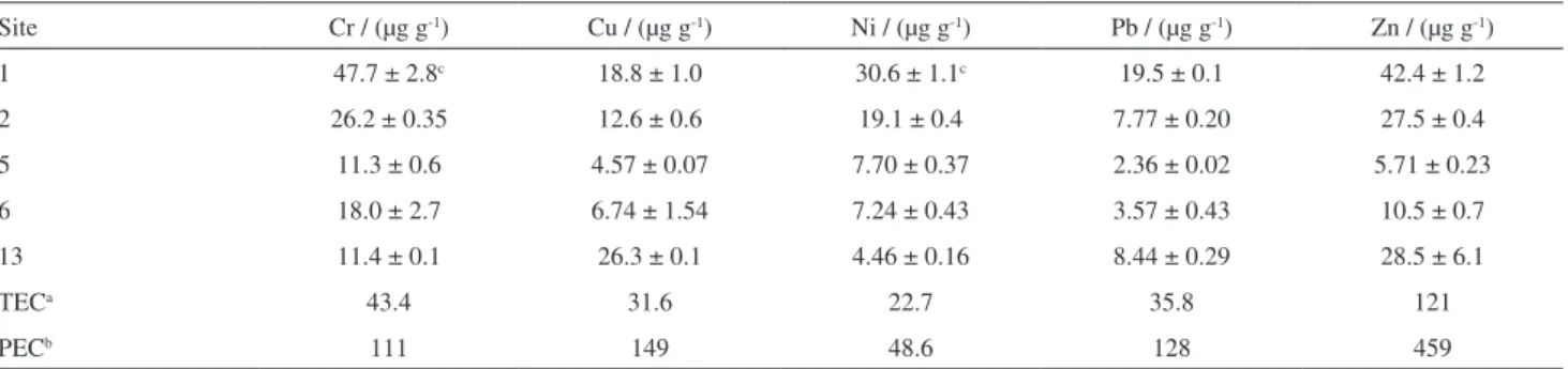
In order to allow assessment of toxicity based on SQG criteria, partial trace metal concentrations were determined following extraction using nitric and hydrochloric acids, which is a procedure compatible with that used in the development of the SQG. Table 5 shows the partial concentrations obtained for each metal, together with the respective PEC and TEC values.
The ranges of metal concentrations found for sites 1, 2, 5, 6 and 13 were (µg g-1): 11.3-47.7 (Cr); 4.57-26.3
(Cu); 4.46-30.6 (Ni); 2.36-19.5 (Pb) and 5.71-42.4 (Zn). For all the sites studied, the values were below the TEC, with respect to the trace metals Cu, Pb, and Zn, indicating that adverse effects on aquatic biota should be unlikely to occur. Cr and Ni showed concentrations superior to the TEC (43.34 and 22.7 µg g-1) at site 1 (47.7 and 30.6 µg g-1),
the ability of TEC to predict adverse effects is lower for Cr and Ni than for the other metals.20 The predictive ability of
the TEC achieved 72% for Cr and Ni, and 82% for Cu, Pb and Zn. This signifies that the probability of the incidence of adverse biological effects at concentrations below the TEC is 28% for Cr and Ni, and 18% for Cu, Pb and Zn.20
It must be emphasized that SQG criteria should be used with caution, as there cannot be any guarantee of a complete absence of toxicity at concentrations lower than the TEC, or that samples where the PEC is exceeded must necessarily be toxic, particularly considering that the SQG were not specifically developed for tropical conditions. For greater confidence, it is important that the results obtained here should be validated using toxicity tests.
Principal component analysis (PCA)
PCA enables data reduction and description of a given multidimensional system by means of a smaller number of new variables. It has been widely applied to identify the sources of metals found in sediments, and to distinguish natural and anthropogenic inputs.3,8,15,16 A data matrix was
constructed using the concentrations of Co, Cr, Cu, Mn, Ni, Pb, Zn, Fe, Al and Corg as columns and the nineteen
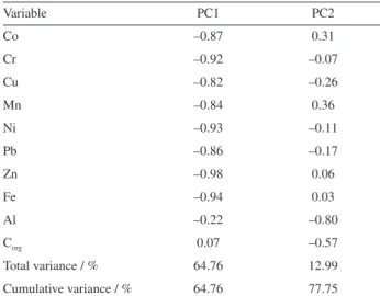
sampling sites as rows (Table 1). PCA was performed on auto-scaled data. The loadings of the original variables in the first two principal components, and the variances explained by each component, are given in Table 6.
The first two principal components were chosen for modeling the data because they described 77.75% of the total variance. The remaining variance probably represented noise, since further principal components did
Table 5. Partial metals concentrations in surface sediments from the Sergipe River Basin (n = 3, mean ± standard deviation), and consensus-based sediment quality guidelines for freshwater sediments20
Site Cr / (µg g-1) Cu / (µg g-1) Ni / (µg g-1) Pb / (µg g-1) Zn / (µg g-1)
1 47.7 ± 2.8c 18.8 ± 1.0 30.6 ± 1.1c 19.5 ± 0.1 42.4 ± 1.2
2 26.2 ± 0.35 12.6 ± 0.6 19.1 ± 0.4 7.77 ± 0.20 27.5 ± 0.4
5 11.3 ± 0.6 4.57 ± 0.07 7.70 ± 0.37 2.36 ± 0.02 5.71 ± 0.23
6 18.0 ± 2.7 6.74 ± 1.54 7.24 ± 0.43 3.57 ± 0.43 10.5 ± 0.7
13 11.4 ± 0.1 26.3 ± 0.1 4.46 ± 0.16 8.44 ± 0.29 28.5 ± 6.1
TECa 43.4 31.6 22.7 35.8 121
PECb 111 149 48.6 128 459
not show any significant variable loadings. The first two principal components showed important loadings for all ten variables, which were therefore all included in the model. The concentrations of Co, Cr, Cu, Mn, Ni, Pb, Zn, and Fe were the dominant variables in the first principal component (PC1), which explained 64.76% of the total variance. Al and Corg showed significant negative loadings in the second
principal component (PC2), which explained 12.99% of the total variance.
It can be seen from the two-dimensional scores plot of PC1 against PC2 (Figure 2) that PCA clearly separated the sampling sites into two groups along the PC1 axis. Group I consisted of sites 1-3, 6, 9 and 10, while group II comprised sites 4, 5, 7, and 11-19. Sediments from the sites in group I (on the left side of the graph) contained the highest concentrations of the trace metals Co, Cu, Mn, Ni, Pb, and Zn, as well as iron. Sites 9 and 10 had estuarine
characteristics, while sites 1-3 and 6 were located in the agriculture region.22 The sites of group II are located to
the right along the PC1 axis. The lowest concentrations of metals were measured for sediments from sites 17-19, which were located in the upper regions of the hydrographic basin where there was little evidence of domestic and/or industrial activities. Other group II sites were located in regions were close to urban areas.22
The high negative loadings of Al and Corg suggest the
existence of a relationship between these species that could have influenced the dispersion of the sites along the PC2 axis. The concentrations of Al and Corg at the different sites
increased from top to bottom in the graph, with evidence for particularly high concentrations of aluminosilicates and organic matter at sites 10 and 19. However, correlation between Al and Corg was not observed for other sites.
Hierarchical cluster analysis (HCA)
HCA, the most common cluster analysis technique used in environmental analysis, identifies groups of samples according to their similarities. HCA is a powerful tool for analyzing data sets to detect both expected and unexpected clusters, including the presence of outliers. This method can be used to group sediments according to their geochemical composition.17-19 The sediment samples from the nineteen
sites were hierarchically clustered on the basis of their normalized metal concentrations. The clusters were generated using Ward’s method with Euclidean distances. The dendrogram obtained contained two distinct clusters (Figure 3). The first cluster, consisting of sites 1-3, 6, 9 and 10, showed approximately 85% dissimilarity with the second cluster. These results were in agreement with those obtained using PCA, and suggest that these six sites
Table 6. Principal component loadings obtained for metals and Corg
Variable PC1 PC2
Co –0.87 0.31
Cr –0.92 –0.07
Cu –0.82 –0.26
Mn –0.84 0.36
Ni –0.93 –0.11
Pb –0.86 –0.17
Zn –0.98 0.06
Fe –0.94 0.03
Al –0.22 –0.80
Corg 0.07 –0.57
Total variance / % 64.76 12.99
Cumulative variance / % 64.76 77.75
Figure 2. Scores graph of PC1 x PC2 applied to Co, Cr, Cu, Ni, Pb, Zn, Fe, Al, and organic carbon concentrations in sediments from the Sergipe River Basin. The groups identified by the analysis are circled.
possessed similar geochemical characteristics, despite being distributed across different regions of the river basin.
Conclusions
The geochemistry of the metals Co, Cr, Cu, Mn, Ni, Pb, and Zn was investigated in surface sediments of the Sergipe River Hydrographic Basin. Iron was shown to be a suitable reference element for definition of a regional geochemical baseline (RGB) for the trace metals. Metals in sediments from sites 3, 4, 7-12 and 14-19 were mainly derived from natural origins, and could be used to define the RGB.
Enrichment factors and geoaccumulation indices were calculated for each metal by dividing its ratio to the reference element by the same ratio found for the RGB. Calculated EF values showed that sediments from sites 1, 5 and 13 could be considered contaminated by Pb, Cr and Cu, respectively. The sediments were classified as unpolluted to moderately polluted, according to the Igeo. A value of Igeo higher than 1
was only obtained for Cu at site 13 (near shipping activities), indicating that there was no large-scale Cu contamination of the sediments of the Sergipe River Basin.
Possible toxicity related to these metals was examined comparing sediment chemical data with TEC-PEC values. Results indicated that adverse effects on aquatic biota should rarely occur, with respect to the trace metals Cu, Pb, and Zn.
PCA clearly separated the sites into two groups: I (sites 1-3, 6, 9 and 10); II (sites 4, 5, 7 and 11-19). HCA confirmed the interpretations made from the PCA results.
Supplementary Information
Supplementary data is available free of charge at http://jbcs.sbq.org.br as PDF file.
Acknowledgments
The authors thank Coordenação de Aperfeiçoamento de Pessoal de Nível Superior (CAPES) and Conselho Nacional de Desenvolvimento Científico e Tecnológico (CNPq) for fellowships, Fundação de Apoio à Pesquisa e à Inovação Tecnológica do Estado de Sergipe (FAPITEC) for financial support (Process 019.203.01714/2010-9), and Instituto Tecnológico e de Pesquisa do Estado de Sergipe (ITPS) for technical support of this study.
References
1. Zhu, L.; Xu, J.; Wang, F.; Lee, B.; J. Geochem. Explor. 2011,
108, 1.
2. Sabadini-Santos, E.; Knoppers, B. A.; Oliveira, E. P.; Leipe, T.; Santelli, R. E.; Mar. Pollut. Bull.2009, 58, 601.
3. Garcia, C. A. B.; Passos, E. A.; Alves, J. P. H.; Environ. Monit. Assess. 2011, 181, 385.
4. Newman, B. K.; Watling, R. J.; Water SA 2007, 33, 675. 5. Tam, N. F. Y.; Yao, M. W. Y.; Sci. Total Environ. 1998, 216, 33.
6. Mil-Homens, M.; Stevens, R. L.; Abrantes, F.; Cato, I.; Environ. Pollut.2007, 148, 418.
7. Acevedo-Figueroa, D.; Jiménez, B. D.; Rodríguez-Sierra, C. J.;
Environ. Pollut. 2006, 141, 336.
8. Garcia, C. A. B.; Barreto, M. S.; Passos, E. A.; Alves, J. P. H.;
J. Braz. Chem. Soc. 2009, 20, 1334.
9. Loring, D. H.; Rantala, R. T. T.; Earth Sci. Rev. 1992, 32, 235. 10. Ianni, C.; Magi, E.; Soggia, F.; Rivaro, P.; Frache, R.;
Microchem. J. 2010, 96, 203.
11. Loring, D. H.; Mar. Chem.1990, 29, 155.
12. Daskalakis, K.; O’Conner, T.; Environ. Sci. Technol. 1995, 29, 470.
13. Aloupi, M.; Angelidis, M. O.; Mar. Environ. Res. 2001, 52, 1.
14. Herut, B.; Hornung, H.; Kress, N.; Cohen, Y.; Mar. Pollut. Bull.
1993, 26, 675.
15. Alves, J. P. H.; Passos, E. A.; Garcia, C. A. B.; J. Braz. Chem. Soc.2007, 18, 748.
16. Passos, E. A.; Alves, J. C.; Santos, I. S.; Alves, J. P. H.; Garcia, C. A. B.; Costa, A. C. S.; Microchem. J. 2010, 96, 50. 17. Idris, A. M.; Microchem. J. 2008, 90, 159.
18. Sakan, S. M.; Dordevic, D. S.; Manojlovic, D. D.; Predrag, P. S.; J. Environ. Manage. 2009, 90, 3382.
19. Saniz, A.; Ruiz, F.; Chemosphere2006, 62, 1612.
20. MacDonald, D. D.; Ingersoll, C. G.; Berger, T. A.; Arch. Environ. Contam. Toxicol. 2000, 39, 20.
21. Passos, E. A.; Alves, J. P. H.; Garcia, C. A. B.; Costa, A. C. S.;
J. Braz. Chem. Soc. 2011, 22, 828.
22. Secretaria de Estado do Meio Ambiente e dos Recursos Hídricos (SEMARH); Diagnóstico Integrado PP-02, Execução dos Serviços para a Elaboração do Plano da Bacia Hidrográfica do Rio Sergipe, 47 p., Technical Report, Aracaju. Sergipe, Brazil, 2010. http://www.semarh.se.gov.br/planosderecursoshidricos acessed in March 2011.
23. Barbieri, E.; Garcia, C. A. B.; Passos, E. D. A.; Aragão, K. A. S.; Alves, J. D. P. H.; Rev. Bras. Ornitol. 2007, 15, 69.
24. Miller, J. C.; Miller; J. M.; Statistic for Analytical Chemistry, 3rd ed.; Ellis Horwood PTR Prentice Hall: London, 1993, pp.
11-120.
25. Farias, C. O.; Hamacher, C.; Wagner, A. L. R.; Campos, R. C.; Godoy, J. M; J. Braz. Chem. Soc. 2007, 18, 1194.
26. Zemberyová, M.; Barteková, J.; Hagarová, I.; Talanta2006, 70, 973.
27. Gomez Ariza, J. L.; Giraldez, U. I.; Sanchez-Rodas, D.; Morales, E.;
28. Gomes, M. V. T.; Costa, A. S.; Garcia, C. A. B. Passos, E. A.; Alves, J. P. H.; Quim. Nova 2010, 33, 2088.
29. Wang, X. S.; Zhu, G. C.; Wang, S. J.; Wan, W. Y.; Tan, Y. B.;
Environ. Monit. Assess. 2011, 177, 263.
30. Jesus, H. C.; Costa, E. A.; Mendonça, A. S. F.; Zandonade, E.;
Quim. Nova2004, 27, 378.
31. Covelli, S.; Fontolan, G.; Environ. Geol.1997, 30, 34. 32. Liaghati, T.; Preda, M.; Cox, M.; Environ. Int.2003, 29, 935. 33. Teng, Y.; Ni, S.; Wang, J.; Niu, L.; Environ. Geol. 2009, 57,
1649.
34. Devesa-Rey, R.; Díaz-Fierros, F.; Barral, M. T.; Microchem. J. 2009, 91, 253.
35. Shevchenko, V.; Lisitzin, A.; Vinogradova, A.; Stein, R.; Sci. Total Environ.2003, 306, 11.
36. Lee, B.; Zhu, L .M.; Tang, J. W.; Zhang, F. F.; Zhang, Y.;
Geochem. J.2009, 43, 423.
37. Liu, W. X.; Coveney, R. M.; Chen, J. L.; Appl. Geochem. 2003,
18, 749.
38. Angelidis, M. O.; Aloupi, M.; Int. J. Environ. Anal. Chem. 1997,
68, 281.
39. Turekian, K.; Wedepohl, K.; Geol. Soc. Am. Bull. 1961, 72, 175. 40. Taylor, S.; Geochim. Cosmochim. Ac.1964, 28, 1273.
41. Mil-Homens, M.; Stevens, R. L.; Abrantes, F.; Cato, I.; Cont. Shelf Res.2006, 26, 1184.
42. Clark, R. B.; Marine Pollution, Oxford University Press: Oxford, UK, 2001.
43. Yaylali-Abanuz, G.; Microchem. J. 2011, 99, 82.
44. Silva, M. R. C.; Honório, K. M.; Brigante, J.; Espíndola, E. L. G.; Vieira, E. M.; Gambardella, M. T. P.; Silva, A. B. F.; J. Braz. Chem. Soc. 2005, 16, 1104.
45. Gimenon-Garcia, E.; Andreu, V.; Boluda, R.; Environ. Pollut.
1996, 92, 19.
46. Muller, G.; Geol. J. 1969, 2, 109.
47. Rubio, B.; Nombela, M. A.; Vilas, F.; Mar. Pollut. Bull. 2000,
40, 968.
48. Zhang, W. G.; Feng, H.; Chang, J.; Qu, J. G.; Yu, L. Z.; Environ. Pollut. 2009, 157, 1533.
49. Davutluoglu, O. I.; Seckin, G.; Ersu, C. B.; Yilmaz, T.; Sari, B.;
J. Environ. Monit.2011, 92, 2250.
50. Harikumar, P. S.; Nasir, U. P.; Mujeebu Rahman, M. P.; Int. J. Environ. Sci. Technol. 2009, 6, 225.
51. Tessier, E.; Garnier, C.; Mullot, J. U.; Lenoble, V.; Arnaud, M.; Raynaud, M.; Mounier, S.; Mar. Pollut. Bull.2011, 62, 2075.
Submitted: April 3, 2012