SCHEMATIC BUS TRANSIT MAPS FOR THE WEB USING GENETIC ALGORITHMS

SCHEMATIC BUS TRANSIT MAPS FOR THE

WEB USING GENETIC ALGORITHMS

II

SCHEMATIC BUS TRANSIT MAPS FOR THE WEB USING

GENETIC ALGORITHMS

Dissertation supervised by

Prof. Dr. Francisco Ramos Romero Dept. Lenguajes y Sistemas Informaticos

Universitat Jaume I Castelló – Spain

Co-Supervised by

Prof. Dr. Angela Schwering Institute for Geoinformatics

Westfälische Wilhelms-Universität Münster Münster – Germany

Dr. Mauro Castelli

Instituto Superior de Estatística e Gestão de Informação Universidade Nova de Lisboa

Lisbon – Portugal

III

ACKNOWLEDGMENTS

"Non Mihi Solum."

I would like to thank first my supervisor and co-supervisors: Francisco Ramos, Angela Schwering and Mauro Castelli. Their trust, help and orientation in the realization of this research was indispensable.

I also leave my most sincere gratitude to the Professors Joaquín Huerta, Michael Gould, Marco Painho, Christoph Brox, and Christian Kray for the excellent organization of the Master of Science in Geospatial Technologies and the thoughtfulness they have with their students.

During this master program I have learned from 18 different Professors. Thank you all for sharing your valuable knowledge. I would like to leave a special memory for Professor Ricardo Quirós Bauset. I will never forget your courage, work and love for life.

My gratitude stays as well with the European Union Commission EACEA for the realization of the Erasmus Mundus Programme. You have given me a unique opportunity to grow as a professional and a human being.

Thanks Dori Apenewicz and Karsten Höwelhans, always kind and helpful. Without your support the pace in this journey wouldn't be the same.

Thanks to my 14 master colleagues that I now call friends. We have spent good times together although, but it was in the difficult ones, far from our families, that your presence was vital. I will never forget you.

From Brazil, I will always be grateful to Professor Pastor Willy Taco, Professor Marcus Lamar, and Professor Clovis Zapata. Your support in this project was crucial.

IV

SCHEMATIC BUS TRANSIT MAPS FOR THE WEB USING

GENETIC ALGORITHMS

ABSTRACT

V

KEYWORDS

Transit Map

Schematic Generalization

Octilinear Graph

Genetic Algorithm

Location-based

Digital Map

Web Visualization

Public Transportation

VI

ACRONYMS

API – Application Programming Interface

GA – Genetic Algorithms

GIS – Geographic Information Systems

OSM– OpenStreetMap

POI – Point of Interest

PT – Public Transportation

REST – Representational State Transfer

SQL – Structured Query Language

SVG –Scalable Vector Graphics

UJI –Universitat Jaume I

UML – Unified Modeling Language

W3C – World Wide Web Consortium

VII

INDEX OF CONTENT

ACKNOWLEDGMENTS ... III

ABSTRACT ... IV

KEYWORDS ... V

ACRONYMS ... VI

INDEX OF TABLES ... IX

INDEX OF FIGURES ... X

1 INTRODUCTION ... 1

1.1 Objectives and delimitations ... 3

1.2 Thesis outline ... 4

2 THEORETICAL REVIEW ... 6

2.1 Public Transportation ... 6

2.2 Public Transportations Maps ... 8

2.3 Graph Theory ... 13

2.4 Graph Algorithms... 15

2.5 Graph Drawing ... 16

2.6 Genetic Algorithms ... 17

3 RELATED WORKS ... 21

4 METHODOLOGY ... 25

4.1 Getting Data Ready ... 25

4.2 Location Based Data retriever ... 33

4.3 Generation of schematic data ... 41

4.4 Web Schematic Data Visualization ... 50

VIII

5.1 Data model and structure analysis ... 53

5.2 Schematization analysis ... 55

5.3 Context and digital-web platform issues ... 58

5.4 Performance issues ... 62

6 CONCLUSION ... 65

IX

INDEX OF TABLES

Table 2.1 Adjacent list example ... 14

Table 2.2 Example of encoding chromosomes. ... 18

Table 2.3 GA crossover example. ... 19

Table 2.4 GA mutation example ... 19

Table 3.1 Summary of researches dealing with the metro map layout. ... 22

Table 4.1 Chromosome genes of path in Figure 4.14 ... 46

Table 4.2 GA Crossover example . ... 47

X

INDEX OF FIGURES

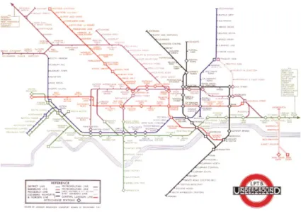
Figure 1.1 First official publication of an octilinear map. Henry Beck 1933. 2

Figure 2.1 Public transportation network components. 7

Figure 2.2 Bus line routes way types (Huang, 2003). 8

Figure 2.3 Example cartographic transit map. 9

Figure 2.4 Example schematic transit map. 9

Figure 2.5 Example of hybrid transit map. 10

Figure 2.6 Variable scaled map of Boston's road map. 13

Figure 2.7 Off-screen objects located by Arrow. 13

Figure 2.8 Simple graph example. 14

Figure 2.9 Graph drawing application example. 16

Figure 4.1 Application data model. 26

Figure 4.2 Line route (blue) vs. Line sequence of stations (red). 27

Figure 4.3 Castellón transit raw data. 29

Figure 4.4 Creation of ghost points to planarize graph. 30

Figure 4.5 Selection of stops in a line route. 31

Figure 4.6 Creation of stations. 32

Figure 4.8 Incoherent line segments positioning. 38

Figure 4.9 Illustration of a spatial creation of influence zone. 40

Figure 4.10 Example of line fragmentation due to spatial influence zone. 41

Figure 4.11 Rational function for fisheye scale distortion. 43

Figure 4.13 London tube map scale variation. 44

Figure 4.14 Example of octilinear path 46

XI

Figure 5.1 Illustration of graph creation after introduction of stations. 54

Figure 5.2 Graph with individual colored line segments for each edge. 54

Figure 5.3 Bus route direction indication. 55

Figure 5.4 Fisheye effect in the network of Castellón. 55

Figure 5.5 Final result after applying the GA for octilinear path schematization. 56

Figure 5.6 GA octilinear schematization with different weights for bend reduction. 58

Figure 5.7 "Less is more". Schematic map information reduction 59

Figure 5.8 Line enhancement by interaction. 60

Figure 5.9 Interaction for seeking information. 61

Figure 5.10 Schematic map and Location-based services. 62

Figure 5.11 Relation generations executed and total execution time. 63

1

1 INTRODUCTION

A public transportation (PT) map is a graphical representation of the geographic elements of the services provided by the PT system. It has as fundamental purpose not only to inform the services available but mainly to allow users to elaborate itineraries using these services to reach a specific location. This kind of information tool is vital for the profusion of the PT system usage since difficulties on elaborate itineraries leads people to choose different means of transportation and by consequence, lacks of transit maps contributes to the underutilization of the services (Allard, 2009).

The metro map layout (Figure 1.1), firstly conceived for the underground network in London, is one of the most famous designs used by cartographers to create transit maps. It is a more diagrammatic representation of the network aimed to enhance connections and sequence of stations in sacrifice of precise geographic information, making it a more efficient information tool for transit needs (Avelar, 2002). Because of this unfaithful geographic representation, the metro map can also be called schematic transit map and we also use the term "octilinear" (Nöllenburg, 2005) for this specific configuration. The octilinear layout is widely used for drawing metro maps network, even though scarce because of its complexity, they are also used for bus network.

2

more pleasant and balanced schematic maps that facilitate the assimilation of information by the user.

Figure 1.1 First official publication of an octilinear map. Henry Beck 1933.

In the past 15 years, researches addressing the automatic metro layout problem have been prolific, and, with the help of growing computer power, the results are every day closer to results of professional handmade maps. This whole context, together with the emerging mobile communication technology, opens new possibilities for the usage of schematic maps.

This research intends to explore the modern mobile devices interactivity and its location awareness as a platform for the use of automatic schematic drawing algorithms. Based on the visual information-seeking "mantra" proposed by Schneiderman (1996), we suggest that maps can be created on demand with minimal information to meet the specific needs of a person or a group and, by interaction, the user can deep in more detailed information. In other words: Personalized interactive schematic maps.

3

Transporte, 2016). The idea behind creating personalized schematic maps consists in selecting only the parts and lines that might be relevant to a specific user in order to have a cleaner and more readable map. Since schematic maps differs from sketched maps by being a more complete source of information for general purposes (Avelar, 2002). We can also call the personalized schematic map as "sketch map" because they are prepared for a specific purpose.

In order to produce personalized schematic maps we assume that the process of producing schematic data must be made in real time. This efficiency in the process is crucial. First, it helps information in the map to be update to the last changes in the operations of the service. Second and more important is that for different areas and different set of lines it is required a different schematic layout. Changes in the area results in changes in scale and in the dimension of the map. Variation in the set of lines implies density variation in the elements on the map. Since an adequate transit schematization depends of dimension, scale and density, a new schematization is required for every personalized map produced.

We aimed our methodology to bus networks because, first, it is the most common model of PT, second, schematic maps are scarcer for this modality, third because bus networks are usually more complex in its morphology and size, in a way that a solution meant for bus should work for metro or others PT means.

We have improved the genetic algorithms (GA) for octilinear schematization developed by Galvao (2010) to generate the schematic data. The GA for path schematization was chosen because of its control over the execution time. To validate the results in a practical case we developed a web application enabling the remote use of the generated schematic maps. Real transit data of Castellón de la Plana (Spain), a typical medium size European city, has been used to produce the final sketches.

1.1

Objectives and delimitations

4

devices. We approach this objective by testing software applications and functionalities that might add extra value to the traditional concept of schematic maps.

The second objective, but as well as relevant, in this project is to identify the advantages and limitations of using genetic algorithms as solution for the automatic generations of schematic maps in real time. To meet this objective we first implemented some of the future work suggestions made by Galvao (2010) to improve the visual quality of the resulting maps and submitted the algorithm to systematic performance test.

It is out of the scope of this project issues related to routing algorithm, journey planner or similar processes. Although some of implemented functionalities depend of this kind of process we opted to use already available external services of directions. It is also out of the scope to develop an algorithm aimed to produce high quality schematic maps similar to the ones made by professional designers. Although, we understand and also work on the concepts of completeness, correctness and elegancy for schematic maps, the main focus of this project is related to schematic map algorithm performance.

1.2

Thesis outline

This research contributes and investigates the computational production and visualization of schematic maps of bus networks for the Web. The structure of the thesis is organized as follow:

Section 2 is theoretical framework required for the development and understanding of the project. It is a brief introduction to the disciplines, techniques and terminology used on the methodology developed.

5

Section 4 is a full description of the methodology from the data preparation, passing through the schematization process itself until the visualization of the schematic data in web. The methodology is always concerning the specificities related to bus networks schematization and interactivity with their components.

Section 5 is the presentation of the results through a novel of the effects of the techniques described in the methodology in the resulting maps. Additionally, it is presented the results of the performance tests made in relation to the schematization process, in special to the GA.

6

2 THEORETICAL REVIEW

2.1

Public Transportation

Transit maps are graphic representation of the main components of a Public Transportation (PT) Network. PT, or mass transit, is a shared modality of transport system that allows the translation of people from one point to another, usually in an urban area on which the vehicle used is owned by third parties. The services might be provided by public or private companies; however it must be available to the general public. The most commons means of public transport are buses, trams, subways, trains or ferries.

According to Vuchic (2005) urban transport influences the shape of cities and their inhabitants' quality of life. Experiments have shown that mass transit has great influence in reduce congestion on urban roads, thus improving the economic, social and environmental traits of a city.

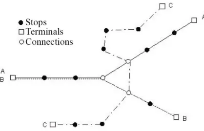
The main component of a PT system is the transport line. The lines are the paths where vehicles travel according to a predefined schedule. A transit line is composed by stops (stations), connections, and terminals. A stop point is a place on the line where the vehicle parks for the landing and boarding of passengers. A connection is a stop that belongs to more than one line. In a connection point, a passenger may perform a transfer from one line to another. Terminal, in this context, can be defined as the start or end stop of a line. A set of transit lines is called network (Vuchic, 2005). Figure 2.1 represents those elements as a network.

2.1.1 Bus Transit Networks

7

Figure 2.1 Public transportation network components.

That way, bus networks have different characteristics in relation to other mass transit systems, and they need to be taken into consideration by professionals that are working on bus transit information systems. Those differences, listed below might not be exclusive for bus systems but they are more evident in it and together represent its peculiarity (Rainsford, 2002).

Bus networks are dynamic: the frequency, shape, or availability of a line can change throughout the day. For example, night bus lines or periodic route change due to urban roads with reversible lanes.

Integration through walk: connection between lines might require a short walk that sometimes includes street crossing, walk around the corner or to another street to board in a different stop point. Connections might contain two or more stop points (not necessarily in the other side of the street).

Roundtrip lacks of equivalence: the outwards and return routes of a bus lines often are partly or totally different. One-way lines are also possible. This differs from metro lines that both-ways can be represented as a single line. Those lacks of equivalence were illustrated by Huang (2003) (Figure 2.2).

8

Figure 2.2 Bus line routes way types (Huang, 2003).

These peculiarities represent challenges on modeling and representing bus networks (Huang, 2003). The following section shows on how designers have been dealing with the graphic representation of transit networks as information tool for passengers.

2.2

Public Transportations Maps

Public transportation maps are informative tools useful not only to make people aware of the available services but crucially to provide information on how to use those services efficiently. In a transit map passengers should be able to identify, first, their origin and destination location and finally decide the line or combination of lines that best fits to reach their final destination. Difficulties on performing this task, i.e., elaborating trip itineraries, promote the underutilizations of the transit services available (Allard, 2009).

Public transportation maps can be conceived in three different topological classes: Conventional cartographic (topographic), schematic (or diagrammatic) and hybrid design.

9

Figure 2.3 Example cartographic transit map (Consorcio Transportes Madrid 2009).

Schematic transit maps (Figure 2.4) intend to be a more conceptual representation of a network. They are designed to be more functional in terms of transit. There is no commitment with scale maintenance and the transit elements are simplified, e.g. lines are straightened. However, the topological connectedness must be preserved. The goal of schematic maps is to provide transit information efficiently by allowing easy identification of connections and easy following the sequence of stops in a path and at any rate are meant to serve for walking reference. The most known schematic transit map format is the octilinear, recognized in the metro map of many cities, and more details on it are given in a separated subsection.

10

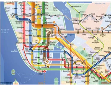
Hybrid design transit maps combine aspects of both, schematic and cartographic (Figure 2.5). In hybrid maps, lines can be straightened and the connectivity highlighted, with simultaneously, being showed together with topographic elements where the general scale of the map keeps mainly constant. Although it is not meant for walking reference, street elements are shown for better localization references. Some hybrid maps designs may be made part schematic and part conventional.

Figure 2.5 Example of hybrid transit map (New York Kick Map 2007).

2.2.1 Schematic Octilinear Maps

The schematic octilinear map, commonly known as the "metro map layout" is the most used diagrammatic format for transit maps. As it was presented previously, it is a functional informative tool for trip elaboration in transit services and it is characterized by having all line segments orientation restrict to vertical, horizontal and both diagonals (octilinear orientations).

11

the same design still being widely used without much modification (Garland, 1994). It turned into a design classic.

2.2.1.1 Rules of Beck's diagram

The most remarkable characteristic of Beck's layout was allowing segments orientated in modulo 45° only, However other common characteristics having been studied and identified in octilinear maps used around. Nöllenburg and Wolff have been listing those rules in the context of automatic drawing of metro maps. The general rule can be listed as follow:

x Do not change the network connectedness topology. It means, the planarity of the network must remains consistent. Extras edge crossings should be avoided. x Restrict edge orientations to the octilinear angles (0°, 45°, 90° 135°, 180°, 225°,

270°, 315° )

x Ensure that adjacent and non-adjacent stations keep a certain minimum distance. And, preferably, keeping distances between adjacent stations as uniform as possible.

x Keep minimal the number of bends along the lines. If bends cannot be avoided, obtuse angles are preferred over acute angles.

x Preserve the relative position between subway stations. For example, a station being north of some other station in reality should not appear below that station on the map.

x Make sure that dense regions of the map get a larger share of the available space. x Color each edge according to the lines to which it belongs. This assumes that each

line has a unique color, and if many lines share a same edge, a parallel for each line must be draw.

x Label stations with their names and make sure that labels do not obscure other labels or parts of the network.

2.2.2 Digital Transit Maps

Digital transit map is the representation of spatial transit information in digital devices. Nowadays, the most used digital devices for passenger looking for transit information are laptops, tablets and smart phones, and in this context, digital maps can also be called mobile maps. Navigation, route finders and other location-based services are consolidated applications for this kind of devices.

12

easy to reproduce, update, edit and personalize and data sets from different source can easily be joined together to create a new map. Digital maps provides new ways of interactions and visualizations and it can be integrated with others services. And, with the emerging of mobile devices, a digital map can now be used on the go.

Together with these benefits new challenges emerged on producing transit maps in the mobile map context. Mobile maps, in contrast with traditional cartography, offer only a small screen to present the necessary information which implies difficulties in presenting the complete information with clarity and readability. Allied to it, despite recent progress, mobile devices have limitations regarding memory, processing and communication bandwidth.

GIModig (2015) addressed the challenge of real-time adaptive generalization of geospatial data to small screen devices (Sarjakoski, et al., 2002). Generalization are functions that simplify, aggregate and reduce geospatial information in map representations and, according Sarjakoski, et al. (2005), those methods are essential in the mobile maps context because increases the readability of information, what is vital for small-display cartography. Others techniques can also be cited as adequate for small display cartography, like angular schematization, fish-eye view and off-screen visualization.

Angular schematization like generalizations, aims to reduce unnecessary information, and emphasizes some aspects of the topology (Avelar, 2002) , thus generating a cleaner, summarized and easy reading map. For this reason it can be used in the context of mobile maps.

13

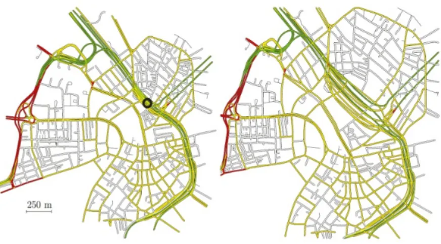
Figure 2.6 Variable scaled map of Boston's road map. (Haunert & Sering, 2011)

Off-screen visualization is a technique that gives indication of off-screen objects locations by cues in form of geometry (arrows, triangles, circles) arranged in the border of the screen which allow users to recognize the locations of the objects outside the limits of the map. This approach allows users to pan and to zoom the map without losing the context of the map viewport and the objects of interest. Figure 2.7 illustrates an example of off-screen object visualization techniques.

Figure 2.7 Off-screen objects located by Arrow. Distance proportional to arrows size. (Burigat & Chittaro,, 2011)

2.3

Graph Theory

Transport networks can be naturally represented as graphs where the vertices represent stop points and the edges the topological connections between the stops.

A simple graph denoted below as G, is a structure formed by two kinds of objects: vertices and edges.

14

Where ܸ represents a finit set of vertices, and we say that |ܸ| =݊. And ܧ represents the set of edges of the graph, and |ܧ| =݉ܽ݊݀ܧ ك ܸ²

One can say that an edge is an unordered pair of vertices. An edge connecting the vertices ݒ and ݓ is denoted simply by ݒݓ or ݓݒ, in this case we say that the edge falls in ݒ or ݓ, and ݒand ݓ are neighbors or adjacent vertices.

The set of all vertices adjacent to vertex ݒ is called neighbors of ݒ, and can be denoted by ܰ(ݒ). The degree of ݒ is ݀(ݒ) = |ܰ(ݒ)|, i. e the number of vertices adjacent to ݒ.

2.3.1 Adjacency list

In graph theory, an adjacency list is a data structure that represents all the edges of a graph in a list. It is a data format for a graph.

Each entry in the adjacency list corresponds to a vertex ݒ in the graph, followed by the set of vertices adjacent to it. The graph in Figure 2.8 can be represented by the adjacency list in the Table 2.1.

Figure 2.8 Simple graph example.

VERTEX ADJACENT VERTICES

A

b, c

B

a, c

C

a, b

Table 2.1 Adjacent list example

2.3.2 Path, cycle and cover

A path ܲ in a graph ܩ is a sequence of distinct vertices (ݒ_଴,ݒ_ଵ, … ,ݒ_௞) of G, such that

ݒ௜ݒ௜ାଵbelongs to ܧ for all ݅ = 0. .݇ െ1. The length of this path is represented by

݈݄݌ = ݇(number of edges). A ݒݓ െ ݌ܽݐ݄ it is a path that starts at ݒ and ends inݓ,

if the ݒݓ െ ݌ܽݐ݄ exists, it means that ݒ and ݓ are accessible. A ݒݓ െ ݌ܽݐ݄ added with the ݒݓ edege i called cycle.

A set ॷ of path and cycles in ܩ is called coverage, if for all ݒ of ܸ_௚, ݒbelongs to at

15

2.4

Graph Algorithms

In order to examine all the vertices and edges of a graph ܩ systematically some graph search algorithm is required. There are several known types of search algorithms. Each search algorithm is characterized by its search strategy of the elements, the order the vertices are visited, the data structure used and the results obtained at the end of the algorithm execution.

2.4.1 Depth-first search

Depth-first search performs a progressive search through expansion of adjacent vertices, and deepens more and more until it encounters a vertex that has no other adjacent vertex that has not yet been visited. So, search goes back to the previous vertex and resumes the search for vertices not yet visited.

As a result, after the execution of the algorithm, all vertices are visited in order that allow the given graph to be divided in a minimum set of paths. This property is especially useful to create a topological data structure of ordered vertices, what is especially useful in the context of this project because it let us treat the graph in separated paths. Algorithm 2.2 is a depth-first search algorithm that makes use of a stack S to control the visited order of the vertices.

1 DepthFirstSearch(G_,r_):

2 create empty stack S

3 i = 0

4 S_.push(r₎

5 while S _{is not empty:}

6 current ₌ S_.pop()

7 if current _{was not visited:}

8 current.order = i++

9 for all _vertex v _{adjacent to current:}

10 S_.push(v₎

16

2.5

Graph Drawing

A convenient way to understand the graph is to represent it geometrically. Graphs drawing deals with the task of representing geometrically a graph to better meet their practical needs. Typically, the obtained drawing should be as readable and clean as possible. The practical value of graph drawing is so pertinent that it owns its unique discipline within the computer graphics field of study.

The graph drawing is motivated by study fields such as topologies organizations, electrical circuits, software engineering, paleontology, sociology and pretty much everything that deals with entities and their relationship (Battista, Eades, Tamassia, & Tollis, 1998). For instance, the Figure 2.9 shows how Arcmap takes advantage of graph drawing to represent models of complex geoprocessing tools.

Figure 2.9 Graph drawing application example.

A drawing Ȟ of a graph ܩ is a function that maps each vertex ݒ of ܩ to a coordinate in a space by Ȟ(v), and the polyline format of each edge ݒݓ of ܩby Ȟ(vw). If no drawing Ȟ(vw) of any distinct edge ݒݓ intersects we say that the drawing Ȟ is planar. If a graph ܩ accepts a planar drawing, we say that ܩ is a planar graph.

17

length of any Ȟ(vw) as uniform as possible, even if the drawing does not accept all the edges to be at the same length, the variance of the lengths must be minimized. Constrains are rules or criteria of the drawing that are applied to only part of the graph, for instance: draw the given path ܲ of ܩ as straight as possible

2.6

Genetic Algorithms

This section is a basic introduction to the concepts of Genetic Algorithms(GA). We use GA in our methodology to simplify paths in octilinear configuration, and the terminology here introduced is used contently in further sections.

Many computational problems require a search for a solution within a wide range of possible solutions (Melanie, 1999). Genetic algorithms (GA) are a search heuristic method for those kinds of problems, suited when optimizations are not implementable or performance is a requirement. The solution found by GA is usually considered an adequate solution, being impossible to prove that it is an optimal solution.

GA are search algorithms inspired by the mechanism of natural selection of Darwin. The basic concept of natural selection is that favorable heritable traits become more common in successive generations of a population, and the less favorable characteristics become less common. Darwin's argument is that individuals with favorable phenotypes are more likely to survive and reproduce than those with less favorable phenotypes, so the genomes associated with favorable phenotypes are in greater numbers in the next generation of a population. Over successive generations, individuals have produced a high degree of adaptation to an ecological niche because their favorable genes passed from their ancestors.

18

This process is repeated until a criteria like found good enough solution or a time limit was reached.

The first and most important step when using a genetic algorithm is to choose how to represent an individual in a population (Melanie, 1999). An individual is the fundamental unit of a genetic algorithm since they represent a possible solution for the given problem.

In genetic algorithms, individuals are referred by the term chromosome, i.e., a set of genes. The most elementary way to encode a chromosome is through a bit string, but depending on the nature of the problem other forms of encoding genomes may be used. Just for illustrative purposes, Table 2.2 shows the representation of two chromosomes encoded in bits string.

NAME GENES CODE

Chromosome ࡭

1011000100110110

Chromosome ࡮

1101111000011110

Table 2.2 Example of encoding chromosomes.

Once the format of a chromosome is defined, an initial population of chromosomes should then be generated to be submitted to the evolutionary process that consists of the following steps:

Evaluation: This step consists in verifying the suitability of chromosomes as a solution to the problem. The evaluation is usually made by a fitness function. The fitness function takes a chromosome as input, and outputs an index used to assess how well the chromosome fits as a solution.

19

Crossover: The crossover process is analogous to the process of chromosomal crossover in the sexual reproduction. It is important to promote the diversity of the individuals in the next population by the exchange of genetic material. This operation consists of two chromosomes recombine randomly generating new chromosomes. Table 2.3 illustrates a crossover between chromosomes and the new generated individuals.

NAME GENES CODE

Chromosome ࡭

10110|00100110110

Chromosome ࡮

11011|11000011110

Chromosome ࡭Ԣ

10110|11000011110

Chromosome ࡮Ԣ

11011|00100110110

Table 2.3 GA crossover example.

Mutation: This operation consists of randomly change some of the genes in the chromosomes. Table 2.4 illustrates the mutation of two chromosomes generated from the crossover in the previous example.

NAME GENES CODE

Chromosome ࡭Ԣ

1011011000011110

Chromosome ࡮Ԣ

1101100100110110

Mutated chromosome ࡭Ԣ

1011010000011110

Mutated chromosome ࡮Ԣ

11111 00100110010

Table 2.4 GA mutation example

Update population: After the selection, crossover and mutation operations are completed, a new set of chromosomes will be created. This step consists on establishing a next generation from this new set of chromosomes.

20

If the test is satisfactory, the process stops, and the best evaluated solution is selected as final solution, otherwise, the GA returns to the evaluation step.

21

3 RELATED WORKS

Computed cartography emerged from the automation of processes usually done manually by cartographers in the past. The evolution of such processes like generalization (line simplification, smoothing, aggregation) are now part of the Geographic Information Systems (GIS) field of study and contributed to the arise of many digital maps tools in the Web, like OpenStreetMaps (OSM) or Google Earth (Allard, 2009). However, digital web maps that provides topological information in schematic layout still scarce.

In the past 15 years many researchers have been made addressing the "The metro layout problem" (Hong, Merrick, & Do Nascimento, 2005). Each research address the problem in a specific way for a specific purpose and the techniques developed are as diverse as possible.

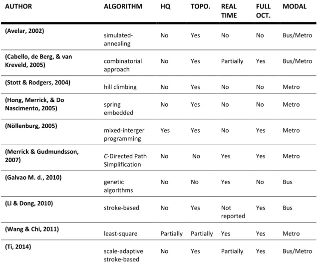
The Table 3.1 lists some authors and their method of schematization. This variety of academic research shows, as said by Allard (2009), how prolific the automatic generations of schematic maps of public transportation has been as a study field.

Each method has its pros and cons. Besides the technique used, we include extra information about the purpose and results obtained. We classify them by the kind of algorithm if it is aimed for high quality maps, if the correct topology is guaranteed, if it's aimed for real time schematization, if all edges are octilinear, and the aimed transport mode. More details and comparison of results can be found in surveys like by Wolff (Drawing subway maps: A survey, 2007) or Nöllenburg (A Survey on Automated Metro Map Layout Methods).

22

AUTHOR ALGORITHM HQ TOPO. REAL

TIME FULL OCT. MODAL (Avelar, 2002) simulated-annealing

No Yes No No Bus/Metro

(Cabello, de Berg, & van

Kreveld, 2005) combinatorial

approach

No Yes Partially Yes Bus/Metro

(Stott & Rodgers, 2004)

hill climbing No Yes No No Metro

(Hong, Merrick, & Do

Nascimento, 2005) spring

embedded

No Yes No No Metro

(Nöllenburg, 2005)

mixed-interger programming

Yes Yes No Yes Metro

(Merrick & Gudmundsson,

2007) C-Directed Path

Simplification

No No Yes Yes Metro

(Galvao M. d., 2010)

genetic algorithms

No No Yes No Bus

(Li & Dong, 2010)

stroke-based No Yes Not reported

Yes Bus

(Wang & Chi, 2011)

least-square Partially Partially Yes Yes Metro

(Ti, 2014)

scale-adaptive stroke-based

No Yes Partially Yes Bus/Metro

Table 3.1 Summary of researches dealing with the metro map layout.

Avelar (Avelar, 2002) presented in her doctoral thesis one of the first complete studies about computational octalinear maps for public transportation. The relevance of this work extends the algorithm in itself. Even being a computational research, important design aspects are covered. Like definitions of schematic maps, map styles classification, symbology conventions and design considerations for aesthetically pleasant maps. Moreover, Avelar handles data modeling aspects essential to the topological characteristics of transports maps and objects of interest.

23

Zurich's road network and having most of the edges in octalinear positions (some edges could not be octalinear placed). However, in terms or performance they were not adequate for real time solutions.

Nöllenburg & Wollf (2006) pushed forward the field of automatic generation of schematic maps. Since they aimed their research to high quality results, their academic works are full of orientations on how to pursue a high level design. Nöllenburg also proved elegantly that the metro layout problem is part of the NP-Complete class of decision problems (Nöllenburg, Automated drawing of metro maps, 2005). It means that the time to solve this problem grows exponentially proportional to the size of the instance. These results drive computer scientist whom deals with the problem to use heuristics searches, treat instances differently, change the definition of the problem, or to use optimizations.

Given this knowledge, Nöllenburg (2006) models the problem in mixed-Integer programming (MIP), a mathematical programming that uses linear and integer constrains. That way, and using a commercial MIP solver design for efficiency (CPLEX), Nöllenburg obtained results of visual quality similar to ones made manually by professional designer. Additionally, his solution was able to create space to label all stations properly. However, even using CPLEX, the execution time cannot be guaranteed to be short, varying from couple of minutes to hours depending on the complexity of the network. More recently, increments on the of the MIP solution, like presented by (Oke & Siddiqui, 2015) succeed on reducing the time of execution.

24

schematization on demand in web, which required real-time solutions. More details on the genetic algorithm will be given in the section 4.3.2.

As it was previously explained, this work does not have as primary objective the development of algorithms to the automatic drawing of schematic maps, instead is about how those algorithms can be availed in the interactive environment of remote web devices like laptops, tablets and smart phones in order to add value to automatic generated personalized maps for bus transit networks. Although the number of publication about algorithm in itself has been substantial, the same doesn't apply to "on the fly" schematic maps.

Swan et al (2007) adapt Avelar's simulated annealing technique to a prototype to generate schematic polylines data as a Web Feature Service (WFS), an Open Geospatial Consortium (OGC) service specification for geometry features. Although the paper lists some practical applications of the web service, nothing is said on how the schematic information can be presented on web clients.

25

4 METHODOLOGY

In Section 2 we have explored fields of study that serve as background for the automatic generations of personalized bus transit maps. From theoretical topics of public transportation, passing through digital cartography and graph theory, the approached topic of this study characterizes itself by being multidisciplinary. This section describes the implementation of the methodology used to obtain the final results. First, we describe the steps to get the data ready to be consulted, second, we describe process related to query the data based on the user given information, then we show the details of the process used to transform the geographic data into schematic data and finally we describe how the schematic data is passed to a web client (browser) and the details of the web client implementation aimed to better present and control the behavior of the schematic.

4.1

Getting Data Ready

This section mainly concerns about relevant issues regarding the treatment of the spatial data necessary to produce schematic data, it means preparing geographic data to represent network topology. We discuss as well concepts specific for bus services map information systems.

4.1.1 Data modeling

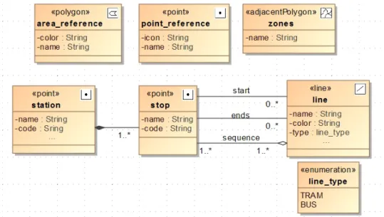
26

Figure 4.1 Application data model.

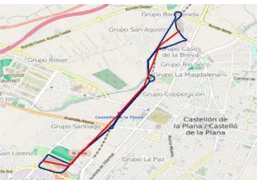
The ݈݅݊݁(paths where vehicles travel according to a predefined schedule) is the main component of a public transportation system. Its main attributes are its name, its color for its visual identification on the map, and its type, that represents the transport model performed in the line, for our case they are bus or tram. The ݈݅݊݁ is also stereotyped as geospatial feature (geometry) line to store the path performed by the vehicles in the transit line. It is worth mentioning that this line geometry is not used to create the final sketched maps at all, but rather the ordinal sequence of stop points is used. Figure 4.2 illustrates the difference between the line route (in blue) and the polyline that connects its sequence of stops (in red).

A transit ݈݅݊݁ is a composition of one or more ordered ݏݐ݋݌ݏ. A ݏݐ݋݌ (place on the line path where the vehicle parks for landing and boarding of passengers) has as attributes its name and code, and its geometry point that indicates its geographic coordinates. It is worth mentioning that this many-to-may relationship between line and stop will produce a third table in the database logical model.

27

sequence of stops of its route until the first stop has been reached again. This way any morphology of bus route can be represented in our data model. In order to identify the end of the outward way, each line is related with a start and end ݏݐ݋݌. The ݏݐ݋݌ point where the line ends, means the end of the outward way. In case of circular lines the start and end ݌݋݅݊ݐ are the same.

Figure 4.2 Line route (blue) vs. Line sequence of stations (red).

Another specific known concept for bus network data model is the concept of the, here called ,ݏݐܽݐ݅݋݊. Called "link" by Rainsford (2002), and differentiates from "route stop" (here stop points) as "bus stop" by Huang (2003), the ݏݐܽݐ݅݋݊ is a set of one or more ݏݐ݋݌. The stops belonging to a same set are within a minimal walk distance ݔ from each other, and a stop is related to one and only one station. Additionally, any two stop of the same station cannot serve in the same line route in consecutively sequence. It means that no vehicle will stop consecutively in two stops belonging to the same station.

The attributes of ݏݐܽݐ݅݋݊ are its name, its code, and its point geometry. The point geometry of ݏݐܽݐ݅݋݊ usually correspond to the geographic coordinates of center of the polygon formed by its ݏݐ݋݌ݏ.

28

data model because stops represent the exactly position of the stops in a route and are useful for locating them in cartographic reference maps, and the station holds the connectivity of the network allowing its integration in a journey planner, the point, as a result, the station geometry is more useful for schematic transit maps.

Line, stop, and station form the group of the essential entities in our data model. The

݌݋݅݊ݐ_ݎ݂݁݁ݎ݁݊ܿ݁ and ܽݎ݁ܽ_ݎ݂݁݁ݎ݁݊ܿ݁, and ݖ݋݊݁ are not essential part of the transit information. However, they are considerable references for sketched maps because they help providing agility to human self location. The ݌݋݅݊ݐ_ݎ݂݁݁ݎ݁݊ܿ݁

has point geometry as attribute because it represents a point feature that can be included in the map, for example, a city hall, a train station, or a cathedral. A point_reference comes as well with its name and a link to icon image as attributes. The area_reference has polygon geometry as attribute, because it represents a polygon feature that can be included in the map, for example, parks, a campus. A

ܽݎ݁ܽ_ݎ݂݁݁ݎ݁݊ܿ݁ come as well with its name and its color as attributes. The ݖ݋݊݁ has the same attributes as ܽݎ݁ܽ_ݎ݂݁݁ݎ݁݊ܿ݁, but they are different entities, ݖ݋݊݁ is a bigger area that delimits city parts as neighborhoods, peripheries, or satellite cities. It is drawn below every other entity in schematic maps and are many times used not only as geographic but as tariff reference for the system.

4.1.2 Data collection

29

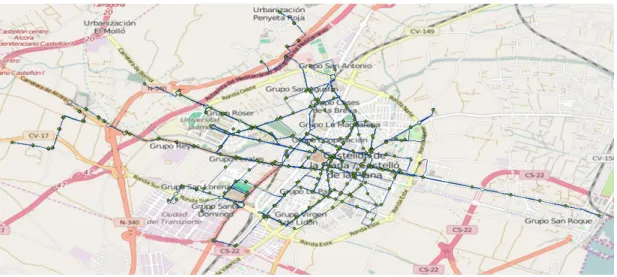
The coordinates of the stops and the polylines of the lines form the set of raw geospatial data necessary for the generations of schematic maps. The Figure 4.3 is the geo visualization of the whole raw data overlaid in an OSM base map. In total are 258 stops (green points) and 20 lines (blue polylines).

Figure 4.3 Castellón transit raw data.

In the next session it is described how to process this data to feed the data model presented in the previous section. It shows how to link the lines with their respective sequence of stops and how to create the stations with their set of stops.

4.1.3 Topological data preparation

With the raw geospatial data (polylines of lines and points of stops) some geospatial process can be performed in order to, first, create the topological order of stops of each line and second, group the stops into stations. Before we proceed to those steps it is important guarantee that the resulting network topology will be planar graph. A planar network is important because facilitates a more precise drawing of network in terms of its topology.

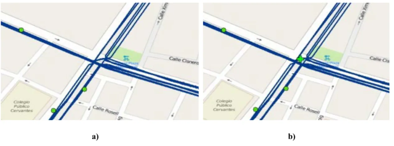
30

green cross, was created to represent topologically this connection between the lines. Those fake stops are set with the name "ghost" to indicate that they should not be represented with a symbol in schematic maps. A total of 19 ghost stops were necessary to be created to guarantee a planar graph, increasing the number of stops from 258 to 277.

a) b)

Figure 4.4 Creation of ghost points to planarize graph.

The next step is the creation of relations between lines and stops (including the ghost ones). The process to relate each line with its sequential group of stops consists of, for each line ݈, selecting from the table of stops, the stops that intersects the polygon route of ݈. The Figure 4.5 illustrates the selected stop points (in cyan) intersected by a specific line. The ids (primary key) of selected stops were used to form a new table that is added with a column with line id that they intersect. A third column with the order of the stops visited by the line on its full route (outward and return) is then added to the table. The tables created by each line are merged to form a new relational table between lines and stops that allow the representation of the connection topology of the transit network. The resulting logical relational model tables are:

LINE( lineId, name, color, vehicletype, polyline, startpointid, endpointid)

STOP (stopId, name, point, stationId)

31

Figure 4.5 Selection of stops in a line route.

The creation of ݏݐܽݐ݅݋݊ is a similar process to the process of identifying connections between lines in journey planning algorithms in transit networks. The stop points within a determined walking distance from each other are grouped, after that, the most distant stops from a same group serving in the same line in a consecutive manner are removed from the group to form an independent station.

32

a) b)

c) d)

Figure 4.6 Creation of stations.

The attribute name of each station was taken randomly from one of its stops. As a result, the station of a ghost stop will also be "ghost". At the end, every stop, including the ghost stops, is associated to one and only one station, and every station is associated with one or more stops. This way a line can be expressed not only as sequence of stops, but as a sequence of stations as well. After this process the total number of stations is 173 (not counting ghosts) against 258 stops. The final resulting logical relational model tables are:

STOP (stopId, name, point, stationId)

STATION(stationId, name, point)

33

others transit entities (although they could be), instead they are present only to server as location references in the schematic maps. It is worth record that geospatial data for those entities were created manually using a GIS with the support of a base map. For the ݌݋݅݊ݐ_ݎ݂݁݁ݎ݁݊ܿ݁ݏ, features as the cathedral, train station, and the general hospital were model. For the ܽݎ݁ܽ_ݎ݂݁݁ݎ݁݊ܿ݁, the features modeled were the central park, the campus, and the Mediterranean Sea. For ݖ݋݊݁, the historical city center, and the boundaries of the city were modeled.

4.2

Location Based Data retriever

In the previous sections was proposed a data model and has been showed how the spatial data can be collected and prepared to feed the data base. This section consists in presenting techniques on how the proposed relational data model can be queried in order to obtain the correct data structure that will enable the production of schematic maps. Retrieve the right data and in the correct other is critical for the quality of the resulting schematic maps.

Bus transit networks are usually bigger and more complex then subway networks. For example the bus network of Wuhan, a 7 million citizen city in China, had 240 bus lines in 2003, and many of routes overlapping each other (Huang, 2003). The creation of an easy to read transit schematic map with all 240 lines is a challenging task even for the most skilled cartographers. For the automatic generation of schematic maps a bigger size of the instances represents more data to be transferred through web, and, especially for schematization, considerable more data to be processed. Moreover, a good readability cannot be guaranteed.

The concept proposed in this work states that the user should receive a minimal but sufficient set of information. Therefore, the data to be transfer and processed will be reduced and the resulting map will become more clear and personalized.

34

of 240 lines be presented to tourist in Wuhan? Digital schematic maps allow us to construct maps with a limited set of information that will attend the needs of an individual. This is more or less the concept of the handmade sketch maps as an alternative to the all-in-one paper maps.

In this section we show an example of how a specific set of lines can be determined to a user. We describe as well how this set of lines is used to query the data base in order to obtain the correct data structure for the generation of schematic maps. Moreover, we introduce a concept of not only reducing the number of lines to be presented, but omitting as well part of the line that are not useful to connect the POIs of the user.

4.2.1 Indentifying lines using Google transit API

To identify the set of lines that are valuable to a user, first, it makes necessary to identify the points of interest (POI) of this user. The POIs are usually locations in the city where the user often goes or intends to go. This data can be obtained from mobile devices in the favorite places stored or current locations of the user for example. The prototype made for this project allows the users to manually add markers to a map indicating their POI. Figure 4.7 exemplifies the selection of three POIs (red markers) by a specific user.

35

Figure 4.7 Selection of POIs.

The routing algorithm is made between the POI. Consequently, the number of POI increases squared the number of requests of routing because it is a simple arrange in two. Since routing algorithms are usually costly processes, is better keeping the number of POIs small. Even the Google API limits the number of routing requests per second.

The lines names found by the routing algorithm are collected and the resulting line set and POIs are the parameters to execute the queries in the database.

4.2.2 Querying Data

The line names and the positions of the POIs are used to form the URI parameters of the HTTP GET method in a REST architecture. The line below exemplify the URI of a GET method containing four lines (L16, L10, L11, L7) and three POIs (Home, Universitat Jaume I and Commercial Center) as parameters.

http://localhost:9080/pubrest/network/x?line=L16&line=L10&line=L11&line=L7&poi=Call e Universitat Jaume I(-0.06737709045410156

39.9937584258632)&poi=Home(-0.04248619079589844 39.988234687450756)&poi=Comercial Center(-0.06325721740722656 39.97955362458796)

36

result in a list of stops, stations, lines, references and zones. In order to have a spatial sequence of the geographic elements the stops, and station lists are queried ordered by the distance of the focal point selected as the city center. This order will imply later in selection order of the schematization algorithm.

The next two necessary data structure required for the schematization are, first, the adjacency list and second, the list of edges.

The list of adjacency represents the connection topology of the network. It shows which stations are direct linked. In other words, an entry in adjacency is a station and its adjacent stations, it means, a list of all pair of stations that are in consecutive order for specific lines.

The query to obtain the adjacency list of stations will be a relational join between a pair of joins between station and stops joined with line. The join between line with the pair station/stop is made by the relational table linestopsequence. Finally to relate stations only with the ones adjacent to them a condition implying consecutiveness must be stated. It means that the difference of the order in a line of their stops must be equal to 1 or െ1. The SQL query below exemplifies this. The final result set is a table with a column with a station id and a column with a station id adjacent to station in the first column. Since line routes overlap each other, this pair of station is grouped in order to avoid repetitions.

SELECT s.id stationid, t.id adjstationid FROM linestopsequence a

JOIN linestopsequence b ON a.lineid = b.lineid JOIN stop x ON a.stopid = x.id

JOIN station s ON x.stationid = s.id JOIN stop y ON b.stopid = y.id JOIN station t ON y.stationid = t.id JOIN line l ON a.lineid = l.id

WHERE (b.sequence = a.sequence - 1 OR b.sequence = a.sequence + 1) AND (s.id <> t.id)

GROUP BY s.id, t.id

37

The other important data structure is the list of edges. The list of edges could easily been obtained from the list of adjacency since an edge is formed by two adjacent stations. However, in the context of schematic transit maps an edge shares one or more line segments and the shared lines by an edge must be identifiable. It means that a segment for each line serving an edge must be drawn in parallel and each segment must be colored with its specific line color.

SELECT s.id stationid, t.id adjstationid, l.id lineid FROM linestopsequence a

JOIN linestopsequence b ON a.lineid = b.lineid JOIN stop x ON a.stopid = x.id

JOIN station s ON x.stationid = s.id JOIN stop y ON b.stopid = y.id JOIN station t ON y.stationid = t.id JOIN line l ON a.lineid = l.id

WHERE (b.sequence = a.sequence - 1 OR b.sequence = a.sequence + 1)

AND ( ST_Distance( ST_GeomFromText('POINT( -0.042666 39.987593)',4326), s.geom) < ST_Distance( ST_GeomFromText('POINT( -0.042666 39.987593)',4326), t.geom) ) ORDER BY stationid, adjstationid

38

A b

Figure 4.8 Incoherent line segments positioning.

The list of relevant lines passed as parameter from the client to the server application should be included as conditions in WHERE statement to limit the records only for those selected lines in the adjacent list query as well as for the edge list query. The SQL line below is an example of how these conditions are included for the set of lines L16, L11, L10 and L7.

...WHERE ... AND ( l.name = 'L16' OR l.name = 'L11' OR l.name = 'L10' OR l.name = 'L7' ) ...

The POIs besides of serving as reference in the final schematic map, they can be used for reducing even more the information to the user. The parts of the lines routes that not connect the POIs are not indispensable to final schematic map. The POIs can be used in the queries to delimit the relevant part of the lines. The next section deals with this issue.

4.2.3 User Influence zone

Most of the time a passenger, while performing a transit journey, uses only part of a transit line. Rarely ever a passenger boards in the start station and leaves in the end station, thus the parts of the line that are not relevant can be omitted from the map. Therefore, the necessary elements to be presented are the paths that connect the POIs, still, a way to identify the start and the end station of each line is important.

39

not being a complete success, it's worth mentioning the details here since some results will be presented with this limitation of the line routes.

SELECT s.* FROM station s, (

SELECT ST_UNION(poisbuffer.geom, stopscircle.geom) AS geom

FROM ( SELECT ST_Buffer(ST_Collect( ARRAY[0.06909370422363281 39.99421871723377)', 4326), 0.04231452941894531 39.98797164114611)', 4326), ST_GeomFromText('POINT(-0.06334304809570312 39.97935631488548)', 4326)] ), 0.012) AS geom ) poisbuffer,

( SELECT ST_MinimumBoundingCircle(ST_Collect( ARRAY[0.06909370422363281 39.99421871723377)', 4326), 0.04231452941894531 39.98797164114611)', 4326), ST_GeomFromText('POINT(-0.06334304809570312 39.97935631488548)', 4326)] )) AS geom

) stopscircle ) poisinfluencearea

WHERE ST_CONTAINS(poisinfluencearea.geom, s.geom)

The spatial solution adopted here consists in using the POIs to construct a polygon that determines the user influence zone. The idea is to select only the geographic transit features contained within this polygon. The polygon that presented the best result was a union of the POIs minimum bounding circle with the buffers of the same POIs. This composition reduces fragmentation of lines because it includes in the influence zone not only the area between the POIs but the area surrounding them as well. Figure 4.9 is a graphical illustration of the influence zone creation and the logical spatial query below exemplifies how to select stations inside the influence zone. In Figure 4.9(c), it is possible to see in cyan the stations selected to be relevant to the user.

40

a)

b)

c)

Figure 4.9 Illustration of a spatial creation of influence zone.

41

Figure 4.10 Example of line fragmentation due to spatial influence zone.

In this section it is presented details about the data structure to generate the schematic maps, additionally, it shows how the data model is queried in order to select only information that is relevant for the user. At the end, the data structures are station list, a stop list, reference list, an adjacency list, and, finally, an edge list. In the next section it is presented how those data structures are used to transform the data into schematic data.

4.3

Generation of schematic data

This section is the core of the methodology. It is where the geographic data is shaped into schematic data. The last section defines and shows how to obtain the data structure that will serve as input for the schematization process. In order to make this transit data attend the desired properties of a schematic map it makes necessary to perform a set of operations that includes conversions, transformations, and generalizations.

42

The conversion from WGS1984 to Cartesian 2D system is an arrangement of the earth surface in a flat surface. This is done by a projection of the ellipsoid into a developable surface and it is a regular operation in cartography that requires a set of trigonometric equations. The conversion used here was held with the support of Java API called JMAPViewer that converts the ellipsoid coordinates to the Mercator projection system.

This conversion is made for all the geographic data and after an affine transformation is performed in order to adjust the origin, scale and rotation of the system to better fit the data in canvas of device screen. The origin of the system is moved to the top left corner of the bounds of the data. The scale is changed to enable the whole data to include in 1000x1000 pixels square. A slight rotation is made in order to make the street lines of Castellón closer to vertical and horizontal grid. This anticlockwise rotation of 16 degrees is not essential but will result in a map with less bends in the transit paths, but the north direction will be changed.

This affine transformation does not change the scale factor of the Mercator projection. It means that the relative distances between the geographic features are preserved. In the next subsection the transformation deals with the variable-scale visualization adequate to schematic transit maps.

4.3.1 Fisheye Transformation

One of the characteristics of schematic transit is that regions with more density of stations get larger share of the available space than regions with less density, i.e., variable scale visualization. This makes the stations to be better distributed in the map and, as result, the space for labels are better distributed making the visualization of the maps more pleasant.

43

Their implementation allows only one focal point and all the data must be inside a determined bound. The equation ݂(ݔ) is an example of a rational function that can be used to calculate the fisheye coordinates of a node. Like illustrated in Figure 4.11, this kind of function indicates how the scale factor is alternated while the distance from focal point grows. The constant c represents the level of distortion to be applied. If c is zero no distortions is applied because linear equations have a constant slope.

݂(ݔ) = (ܿ כ ݔ + ݔ) /(ܿ כ ݔ + 1)

Figure 4.11 Rational function for fisheye scale distortion.

Using the most congested area of Castellón (center) as focal point, all the spatial data is submitted to a fisheye transformation. The impact on the scale factor throughout the limits of the data bounds can be visualized in as Figure 4.12 (Sarkar & Brown, 1994).

44

Figure 4.12 Fisheye scale distortion effect.

Ti & Li (2014) developed a schematization algorithm that is able to identify automatically the congested areas and, in addition, a multi focal fisheye transformation is executed through the spatial data. This approach is more adequate to automatic drawing of schematic maps because it reduces the dependency of human interference and, because it is multi focal, it allows a better distribution of stations in metropolis composed with satellites cities. However, Ti & Li didn't present the detail of the execution time of their transformations algorithms and it is not possible to affirm how its computational cost will affect real time schematizations.

45

4.3.2 Octalinear Path Simplification using Genetic Algorithms

The goal on this dissertation is to explore the use of automatic generation of schematic maps into real time web applications in order to produce customized schematic maps. Since the metro layout problem has been proven to be NP-Hard (Nöllenburg, 2005) and, by a consequence, optimal solutions for the problem still a very timing consuming task, we opted to adopt a path octilinear schematization solution that uses genetic algorithms to reduce the bend along the path, limiting its distortion in relation to its original shape. Although path schematization approaches to the metro layout problem does not guarantee the topological correctness in the resulting layout, this constrain was sacrificed for performance purposes, since the combination of preserving the topology, octilinear layout, and bend reduction is responsible for the NP-Hardness of the problem.

In spite of not guarantee the correct topology, the algorithm tends to avoid distortions (distance) in the resulting layout. It means that the topology of the original input is used as information for some topology correctness in the output. That, allied to the fact that instances tend to be small, in the specific case here, contributes to reduce the topological rupture in the final layout.

Path schematization requires first that the transit graph must be disjoint into non-overlapping paths that cover the whole graph. To obtain a minimal set of paths, a depth-first search algorithm is performed in the network. The resulting set of path is, then, sent to be schematized by the GA, and a new schematic position for each station is calculated.