Time forecast of a break-off event from a hanging glacier

(1)

TCD

9, 4925–4948, 2015

Prediction of glacier break-off J. Faillettaz et al.

Title Page

Abstract Introduction

Conclusions References

Tables Figures

◭ ◮

Back Close

Full Screen / Esc

Printer-friendly Version

Interactive Discussion

Discussion

P

a

per

|

Discussion

P

a

per

|

Discussion

P

a

per

|

Discussion

P

a

per

|

The Cryosphere Discuss., 9, 4925–4948, 2015 www.the-cryosphere-discuss.net/9/4925/2015/ doi:10.5194/tcd-9-4925-2015

This discussion paper is/has been under review for the journal The Cryosphere (TC). Please refer to the corresponding final paper in TC if available.

Time forecast of a break-o

_ff

event from

a hanging glacier

J. Faillettaz1, M. Funk2, and M. Vagliasindi3

1

3G, UZH, University of Zürich, Zürich, Switzerland

2

VAW, ETHZ, Zürich, Switzerland

3

Fondazione Montagna Sicura, Courmayeur, Aosta Valley, Italy

Received: 5 August 2015 – Accepted: 1 September 2015 – Published: 17 September 2015

Correspondence to: J. Faillettaz ([email protected])

(2)

TCD

9, 4925–4948, 2015

Title Page

Tables Figures

◭ ◮

Back Close

Full Screen / Esc

Discussion

P

a

per

|

Discussion

P

a

per

|

Discussion

P

a

per

|

Discussion

P

a

per

|

Abstract

A cold hanging glacier located on the south face of the Grandes Jorasses (Mont Blanc, Italy) broke off on the 23 and 29 September 2014 with a total estimated ice volume of 105 000 m3. Thanks to very accurate surface displacement measurements taken right up to the final break-off, this event could be successfully predicted 10 days in

ad-5

vance, enabling local authorities to take the necessary safety measures. The break-off

event also confirmed that surface displacements experience a power law acceleration along with superimposed log-periodic oscillations prior to the final rupture. This pa-per describes the methods used to achieve a satisfactory time forecast in real time and demonstrates, using a retrospective analysis, their potential for the development

10

of early-warning systems in real time.

1 Introduction

Rockfalls, rock instabilities due to permafrost degradation, landslides, snow avalanches or avalanching glacier instabilities are gravity-driven rupture phenomena occurring in natural heterogeneous media. Such events have a potential to cause major disasters,

15

especially when they are at the origin of a chain of processes involving other ma-terials such as snow (snow avalanche), water (flood) and/or debris (mudflow). The reliable forecasting of such catastrophic phenomena combined with a timely evacua-tion of the endangered areas is often the most effective way to cope with such natural hazards. Unfortunately, accurate time prediction of such events remains a somewhat

20

daunting task as (i) natural materials are heterogeneous, (ii) the heterogeneity is dif-ficult to quantify and measure, and (iii) the rupture is a non-linear process involving such heterogeneities. Although often located in a remote high-mountain environment, avalanching glacier instabilities offer an interesting starting point for investigating early-warning perspectives of break-offevents, as a glacier consists of a unique material (ice)

25

(3)

TCD

9, 4925–4948, 2015

Title Page

Tables Figures

◭ ◮

Back Close

Full Screen / Esc

Discussion

P

a

per

|

Discussion

P

a

per

|

Discussion

P

a

per

|

Discussion

P

a

per

|

be placed on the rupture processes leading to the initiation of the instability. Recently, considerable efforts in monitoring, analyzing and modeling such phenomena have led to significant advances in understanding the destabilization process and in improving early-warning perspectives (Faillettaz et al., 2015).

In general, it is possible to distinguish three types of avalanching glacier

instabili-5

ties according to the thermal properties of their ice/bedrock interface (Faillettaz et al., 2011b, 2012, 2015). If temperate or polythermal, the presence of liquid water in the glacier plays a key role in the initiation and the development of the instability as its presence influences the basal properties of the ice/bedrock interface (diminution of friction, lubrication or loss of support). In such cases, several preliminary conditions to

10

be fulfilled can be identified, but an accurate time forecast of an impending break-o_ff event is still far from being possible. If the ice/bed interface is partly temperate, the presence of melt water may reduce the basal resistance, which promotes the instabil-ity. No clear and easily detectable precursory signs are known in this case, and the only way to infer any potential instability is to monitor the temporal evolution of the

15

thermal regime. If the ice/bedrock is cold, glaciers are entirely frozen to their bedrock. This situation appears in the case of high altitude hanging glaciers located entirely in accumulation zone. The snow accumulation is mostly compensated by periodic break-offof ice chunks (Pralong and Funk, 2006), occurring once a critical point in glacier geometry is reached. The instability results from the progressive accumulation of

in-20

ternal damage due to an increasing stress regime caused by glacier thickening. In this case, the rupture occurs within the ice, typically a few meters above the bedrock. The maturation of the rupture was shown to be associated with a typical time evolution of both surface velocities (Faillettaz et al., 2008) and passive seismic activity (Faillettaz et al., 2011a). This characteristic time evolution can theoretically be used to predict the

25

occurrence of a catastrophic event. This was done a posteriori with data obtained prior to the 2005 break-offof the Weisshorn glacier.

(4)

TCD

9, 4925–4948, 2015

Title Page

Tables Figures

◭ ◮

Back Close

Full Screen / Esc

Discussion

P

a

per

|

Discussion

P

a

per

|

Discussion

P

a

per

|

Discussion

P

a

per

|

to major ice avalanches that occasionally reached as far as the valley. In autumn 2008, the glacier recovered its previous critical geometry from the year 1998 and a crevasse opened in the lower part of the tongue, prompting the local authorities to initiate a mon-itoring program to enable a time forecast of the expected break-offevent. The glacier finally broke offcausing no damage in autumn 2014, after more than 5 years of

moni-5

toring. The break-offwas successfully predicted 2 weeks in advance.

The aim of this paper is to confirm the validity of the time forecast procedure first developed in 2005 on the Weisshorn glacier and to apply it here in real time.

After describing the glacier and the monitoring system installed on the glacier, we analyze the time evolution of the surface displacement measurements in the context

10

of a time forecast procedure. While comparing this break-o_ffevent with the Weisshorn glacier break-offevent of 2005 we discuss the results obtained, with the goal of improv-ing the understandimprov-ing of this phenomenon.

2 Grandes Jorasses glacier

2.1 Study site

15

The Whymper glacier (Fig. 1) is located on the south face of the Grandes Jorasses (Mont Blanc massif, Italy) between 3900 and 4200 m a.s.l. (Fig. 1). This very steep cold hanging glacier lies above the village of Planpincieux and the Italian Val Ferret, a fa-mous and highly frequented tourist destination both in winter and summer. Historical data and morphological evidence indicate that the glacier experienced recurrent

break-20

(5)

TCD

9, 4925–4948, 2015

Title Page

Tables Figures

◭ ◮

Back Close

Full Screen / Esc

Discussion

P

a

per

|

Discussion

P

a

per

|

Discussion

P

a

per

|

Discussion

P

a

per

|

2.2 Break-offevent history

The glacier broke offseveral times during last 100 years. Some of these events have been observed and reported:

– On 21 December 1952, after an intensive snowfall period, a huge avalanche was released below the Grandes Jorasses which destroyed a 200 year old

for-5

est and blocked the bottom of the Val Ferret over a distance of more than 1 km. The avalanche volume was estimated at more than 1 000 000 m3. It is not clear whether the snow avalanche was triggered by an ice avalanche from the Whym-per glacier.

– In August 1993 and July 1996, the glacier released ice avalanches of 80 000 and

10

24 000 m3, respectively. These ice avalanches did not reach the valley.

– The last major break-off event occurred in the night of 31 May to 1 June 1998. Almost the entire Whymper glacier (around 150 000 m3) broke offat one time and the triggered ice avalanche reached the bottom of the valley, fortunately without causing damage.

15

In the following years, the hanging glacier has progressively re-formed, as it is located in an accumulation area. Ten years later, in 2008, the glacier almost recovered its 1998 geometry. In autumn 2008 a crevasse opened at the lower part of the glacier, prompting the local authorities to initiate a monitoring program.

2.3 Present monitoring: 2009–2014

20

(6)

TCD

9, 4925–4948, 2015

Title Page

Tables Figures

◭ ◮

Back Close

Full Screen / Esc

Discussion

P

a

per

|

Discussion

P

a

per

|

Discussion

P

a

per

|

Discussion

P

a

per

|

be monitored. Because of instrument problems, the seismic activity unfortunately could not be monitored as initially planned.

Starting in 2010, surface displacements were continuously recorded at several stakes at 2 h intervals (if the prisms were visible, i.e., in good weather conditions) with the aim to detect an impending ice avalanche in a timely manner (Margreth et al., 2011).

5

Using the same correction technique as described by Faillettaz et al. (2008), the sur-face displacements could be determined with an accuracy better than 1 cm, allowing surface velocities to be inferred.

In parallel to the monitoring program, a safety concept for the valley floor was devel-oped considering several scenarios of falling ice volumes. The different ice avalanche

10

scenarios were simulated using the 2-dimensional calculation model RAMMS. The nec-essary safety measures were defined according to the local avalanche danger level and the potential volume of a break-offevent (Margreth et al., 2011).

2.4 The 2014 break-offevent

From 2010 on, surface displacements were surveyed without interruption. The

Whym-15

per glacier finally broke offwith an estimated ice volume of same order of magnitude as the 1998 event (about 105 000 m3). Contrary to the 1998 event, the glacier broke o_ffin two events on 23 and 29 September 2014, without reaching the valley (Fig. 1). At the final break-off, 4 reflectors were still active, 2 of them in place for more than 2 years. Despite poor weather conditions between the 16 and 21 September, the

mon-20

(7)

TCD

9, 4925–4948, 2015

Title Page

Tables Figures

◭ ◮

Back Close

Full Screen / Esc

Discussion

P

a

per

|

Discussion

P

a

per

|

Discussion

P

a

per

|

Discussion

P

a

per

|

3 Results

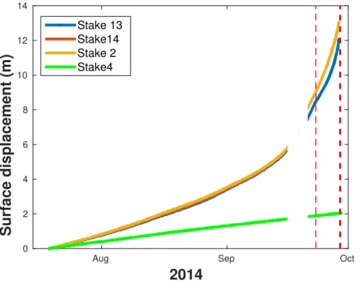
Figure 2 shows the corrected surface displacements and Fig. 3 the associated de-rived surface velocities of the 4 stakes (Fig. 1) prior to the break-off. The assocated derived surface velocities are computed taking the surface displacements interpolated on regular time step and smoothed on 5 points. Note that Stakes 13 and 14 have more

5

than 2 years of nearly continuous measurements, the position of Stake 13 having been measured up to the final break-offevent on 29 September. The accuracy of the mea-surements was less than a centimeter (Faillettaz et al., 2008). Note that this constitutes a unique dataset not only because of the great accuracy and long measurement period but also due to available surface displacement measurements up to a few hours prior

10

to the break-off event. Whereas the motion of Stake 4 is constant (Fig. 2), the three other prisms show a clear acceleration prior to break-off.

3.1 Previous findings on cold glacier break-off

These observations exhibit striking qualitative analogies with those of the 2005 Weis-shorn event (Faillettaz et al., 2008).

15

1. This steep cold hanging glacier experiences periodic break-offevents.

2. The geometrical configuration of the glacier is similar before each break-off.

3. An upper crevasse spanning the whole glacier marks a clear distinction between a stable upper part (where Stake 4 is located) and a downstream unstable part (where the other reflectors were located, Fig. 3). A crude estimation of the volume

20

of the unstable part is thus possible.

(8)

TCD

9, 4925–4948, 2015

Title Page

Tables Figures

◭ ◮

Back Close

Full Screen / Esc

Discussion

P

a

per

|

Discussion

P

a

per

|

Discussion

P

a

per

|

Discussion

P

a

per

|

5. The rupture did not occur at the ice/bedrock contact but a few meters above it, within the ice (Fig. 1).

6. The total break-offoccurred on two occasions; a minor side section of the glacier was released first.

Based on a retrospective analysis, the main conclusion drawn by Flotron (1977) and

5

Röthlisberger (1981) was that the forecast of a break-offoccurrence was possible using surface displacements alone. The principle is to fit the characteristic acceleration of the surface displacements with a power law behavior of the form:

s(t)=s₀+u_st−a(tc−t)θ, (1)

wheres(t) is the displacement (in meters) at timet (in days),s0 a constant in meters, 10

us the constant velocity of the upstream part (in m d− 1

), tc the critical time (in days),

θ <0 (without units) and a (in m d−θ_{) the parameters characterizing the acceleration.}

In this way, the critical timetc, i.e., time at which the theoretical displacement becomes

infinite, could be evaluated simply using such empirical law. Although break-o_ffwould necessarily occur earlier, this critical time represents the upper limit of the break-off

15

timing.

Moreover, an oscillating pattern superimposed on the power law acceleration of the surface displacements was evidenced prior to the 2005 Weisshorn event (Pralong et al., 2005; Faillettaz et al., 2008). Such behavior was shown to be log-periodic oscil-lating behavior superimposed on this acceleration (for appearance and interpretation

20

see Faillettaz et al., 2015). The time evolution of the surface displacement measure-ments can be described with the following equation (after Sornette and Sammis, 1995; Pralong et al., 2005):

s(t)=s0+ust−a(tc−t)θ "

1+Csin2πln(tc−t)

ln(λ) +D

#

(9)

TCD

9, 4925–4948, 2015

Title Page

Tables Figures

◭ ◮

Back Close

Full Screen / Esc

Discussion

P

a

per

|

Discussion

P

a

per

|

Discussion

P

a

per

|

Discussion

P

a

per

|

whereC the relative amplitude (without units), λ the logarithmic frequency (in days) andDthe phase shift of the log-periodic oscillation (without units).

Note that such oscillating behavior was also evident prior to the 2014 Whymper glacier break-off, as such oscillating patterns are clearly visible on the derived velocity without post-processing (Fig. 3).

5

3.2 Application to forecasting

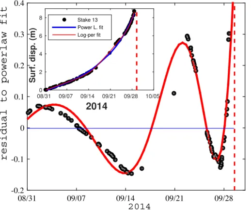
Previous findings were applied in order to forecast the break-offin real time. As soon as a significant increase in velocity was detected, the same procedure was followed as in Faillettaz et al. (2008). We periodically fitted surface displacements of all stakes to a power law (Eq. 1) and a log periodic oscillating behavior (Eq. 2). Figure 4 shows the

10

residuals to the power law fit for two points (Stakes 13 and 14) using the last month of data to 16 September; Table 1 contains the values of the parameters in Eq. (2), taking λ=2 d. Note that measurements are available up to the final break-off for 3 prisms (i.e., Stake 13, Stake 2 and Stake 4) and stopped on 16 September for Stake 14, i.e., 8 days before the first break-off. It appears that the power law describes well

15

the surface displacements with an accuracy of about 5 cm, about the same order of magnitude as the one observed during the 2005 Weisshorn event. However, residuals show an oscillating pattern. When using the log-periodic function (Eq. 2), the fit (shown in red) becomes significantly better, with an accuracy of the order of magnitude of the measurement accuracy (less than a centimeter). Results show that the critical time

20

ranges between 1 and 4 October, which is fairly close to the observed break-o_ff. However, even if Stake 14 is located on a section that broke offearlier, no significant differences could be detected. Our approach is not able to detect whether the break-off

would happen all at once or could occur as successive small break-o_ffs.

Now when investigating the entire dataset for Stake 13 (where measurements were

25

(10)

TCD

9, 4925–4948, 2015

Title Page

Tables Figures

◭ ◮

Back Close

Full Screen / Esc

Discussion

P

a

per

|

Discussion

P

a

per

|

Discussion

P

a

per

|

Discussion

P

a

per

|

(Fig. 5)! Such a broad oscillating pattern had never been observed before, confirming that the jerky motion of the glacier (with oscillating nature) has a physical origin.

4 Discussion

4.1 Appearance of log-periodic behavior

Faillettaz et al. (2011a, 2015) explain the origin of the log-periodic oscillating behavior

5

as the result of a Discrete Scale Invariance, a weaker kind of scale invariance accord-ing to which the system obeys scale invariance only at a specific scalaccord-ing factor scale (Sornette and Sammis, 1995; Sornette, 1998; Zhou and Sornette, 2002a; Sornette, 2006). This partial breaking of the continuous symmetry is a result of the dynamic in-teractions between newly developed micro-cracks, as shown by Huang et al. (1997)

10

and Sahimi and Arbabi (1996).

To identify the log-frequency, we analyzed the data in the same way as Faillettaz et al. (2008) with a Lomb periodogram analysis (Press, 1996; Zhou and Sornette, 2002b), which is designed to analyze non-uniformly sampled time series. This method enables us to determinefLomb as a function of cos(2πfLombt). The parameter λin Eq. (2) can 15

then be evaluated easily as λ=e1/fLomb_{. Unfortunately, the critical time} _t

c has to be

known to perform this analysis, i.e., this analysis can only be an a posteriori analysis. It clearly shows (Fig. 6a) peaks in Lomb power (power spectral density) atλ∼2 d for

the three analyzed points, confirming that the oscillating behavior is not a measure-ment artefact but has physical origins, such as the merge of newly developed

micro-20

cracks. Note that another strong log frequency appears atλ∼7.4 d for Stakes 2 and

13 (Fig. 6b), after the first break-off. The reason for the appearance of such peak is not clear but is probably induced by the occurrence of the first break-offthat changes the geometry of the glacier: Using experimental data, Moura et al. (2005, 2006) suggested that grain size and loading rate directly influence log-periodic oscillations. A possible

25

(11)

TCD

9, 4925–4948, 2015

Title Page

Tables Figures

◭ ◮

Back Close

Full Screen / Esc

Discussion

P

a

per

|

Discussion

P

a

per

|

Discussion

P

a

per

|

Discussion

P

a

per

|

loading of the remaining section of the glacier, i.e., loading rate change, introducing then another subharmonic log frequency and perturbing the overall behavior of the remaining section of the glacier where Stakes 2 and 13 stand.

4.2 Power law vs. log-periodic

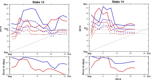
Besides a more accurate fit (Figs. 4 and 5), Fig. 7 (bottom) shows that errors (given

5

as 95 % confidence interval) in the determination of the critical timetc are generally

smaller for periodic fit than power law fit, confirming once again a more reliable log-periodic fit. Usually power law evaluates a larger (later) critical time than log-log-periodic law.

4.3 Accurate determination of break-offoccurrence

10

As critical timetcgiven by power law or log-periodic fit indicates time at which surface

displacements are theoretically infinite, real break-offis expected beforetc. When fitting

in real time the surface displacement with both power law and log-periodic behavior, it is not only possible to assess the critical time but also the time at which the derived velocities are expected to reach a given threshold (for example 50 cm d−1_{or 1 m d}−1_).

15

Fitting and estimating the time at which the associated velocity reaches a given thresh-old provides a more accurate way to predict the real break-off. We developed a software based on this idea by fitting in real time the measurements with both power law and log-periodic behavior and thus provide an estimate of the break-offtime.

From our knowledge, it is not possible to know in advance the velocity at which

break-20

offwill occur. However, from previous events (Weisshorn 1973 and 2005 event, Flotron, 1977; Röthlisberger, 1981; Faillettaz et al., 2008), it seems that break-off occurs be-tween 50 cm d−1_{to 1.2 m d}−1_{, but this is based on a restricted number of events.}

Taking threshold surface velocities of 50 cm d−1_{and 1 m d}−1_{, our analysis performed}

every days from the 12 to 16 September suggested that break-o_ffcould occur between

25

the 23 September (vth=50 cm d− 1

) and the 29 September (vth=1 m d− 1

(12)

TCD

9, 4925–4948, 2015

Title Page

Tables Figures

◭ ◮

Back Close

Full Screen / Esc

Discussion

P

a

per

|

Discussion

P

a

per

|

Discussion

P

a

per

|

Discussion

P

a

per

|

method provided the exact timing of the real break-offs, around 10 days in advance. Following this analysis, alert was immediately sent to the authorities leading them to close the endangered area one week before the event. Note that the definition of the velocity threshold has an influence on the prediction itself, as we saw nearly one week is needed for the glacier to accelerate from 50 cm d−1_{to 1 m d}−1_{. The precise prediction}

5

would also not only be based on a correct fit of the surface displacement data but also on a guess of this parameter. We suggest to choose 40 cm d−1_{as a conservative}

threshold to define a high break-offdanger time zone.

4.4 How much in advance can be the break-offpredicted?

Surface displacement was analyzed retrospectively based on the last month of data for

10

each prism, and the critical time as well as the time at which the fitted velocity reached 50 cm d−1 ₍_v

50) and 1 m d− 1

(v100) were plotted as a function of the time of analysis

(Fig. 7). Associated errors (Fig. 7 bottom) account for the fitting procedure.

First, the prediction is better using log-periodic fit than power law fit. This retro-spective analysis shows that the prediction is correct after 12 September, i.e., 11 and

15

17 days before the break-offwith a confidence interval becoming less than than 10 days for log-periodic fit.

This analysis points out the great prediction potential – and early warning perspec-tives – of this method, as the exact time of the break-off could be forecast almost 2 weeks before its occurrence. Note that both power law and log-periodic fits become

20

less accurate after the first break-o_fffor Stake 13. Such e_ffect might be related to the sudden change in glacier geometry that may influence surface displacements at Stake 13. However, note that time at which estimated derived velocity reaches 1 m d−1₍_v

100)

(13)

TCD

9, 4925–4948, 2015

Title Page

Tables Figures

◭ ◮

Back Close

Full Screen / Esc

Discussion

P

a

per

|

Discussion

P

a

per

|

Discussion

P

a

per

|

Discussion

P

a

per

|

5 Conclusions

Grandes Jorasses glacier broke offtwice, on 23 and 29 September 2014. In 2008, as it was suspected that this glacier becoming unstable, a long-term monitoring program was initiated. At the time of the break-o_ff, 4 prisms spread over the glacier enabled surface displacements to be measured in a very accurate way up to the time of the

5

break-off. By regularly analyzing the dataset, it was possible to forecast the event ten days in advance, enabling local authorities to close offthe endangered areas and thus prevent catastrophic outcomes.

It was possible to confirm definitely that surface displacement exhibits strong log-periodic oscillating behavior superimposed on a global power law acceleration prior to

10

its break-off, as first discovered for the Weisshorn event (Faillettaz et al., 2015). In the immediate vicinity of the break-off, such oscillations reached an amplitude of more than 40 cm, almost one order of magnitude larger than revealed in previous findings. By fit-ting surface displacements to this behavior, the critical time, i.e. time at which surface displacement become infinite, can be determined. The surface velocities at the two

15

events were 0.5 and 1.2 m d−1_{, in the same range as for the Weisshorn event,}

suggest-ing that break-off of a cold hanging glacier could occur as soon as surface velocities reached 0.5 m d−1_{. By taking critical time as an upper time bound of the event}

occur-rence, this method provides a good estimate of the timing of the break-off. We showed that evaluating the time at which extrapolated velocities (based on the log-periodic fit)

20

reach a given threshold (0.5 and 1 m d−1_{) provides a significantly better forecast.}

How-ever, in the present case, the time needed for the glacier to increase its velocity by 50 to 100 cm d−1_{was in the order of a week. In practice, we suggest that}_v

=0.4 m d−1_be

ap-plied to determine the period of highly probable break-offoccurrence. A retrospective analysis based on this method showed that an accurate prediction of the phenomenon

25

can be made two weeks before its occurrence using the last month of surface displace-ment data and 0.5 and 1 m d−1_{as velocity thresholds. Although the crude volume can}

(14)

TCD

9, 4925–4948, 2015

Title Page

Tables Figures

◭ ◮

Back Close

Full Screen / Esc

Discussion

P

a

per

|

Discussion

P

a

per

|

Discussion

P

a

per

|

Discussion

P

a

per

|

this method does not seem to be able to detect whether the break-off will occur as a single large event or as a series of smaller events, as no differences in the evolution of surface displacements were detected. This has of course important consequences for risk evaluation, as the resulting ice avalanche (and also the chain of processes re-sulting from its release) depends on the initial ice volume released. To conclude, our

5

results suggest that the present methods exploiting the log-periodic oscillating behavior are universal and thus can be applied in real time to forecast a break-offon any cold unstable hanging glacier.

Acknowledgements. The authors thank Susan Braun-Clarke for proofreading the English.

References

10

Faillettaz, J., Pralong, A., Funk, M., and Deichmann, N.: Evidence of log-periodic oscillations

and increasing icequake activity during the breaking-offof large ice masses, J. Glaciol., 54,

725–737, doi:10.3189/002214308786570845, 2008. 4927, 4930, 4931, 4932, 4933, 4934, 4935

Faillettaz, J., Funk, M., and Sornette, D.: Icequakes coupled with surface displacements for

15

predicting glacier break-o_ff, J. Glaciol., 57, 453–460, doi:10.3189/002214311796905668,

2011a. 4927, 4934

Faillettaz, J., Sornette, D., and Funk, M.: Numerical modeling of a gravity-driven instability of

a cold hanging glacier: reanalysis of the 1895 break-offof Altelsgletscher, Switzerland, J.

Glaciol., 57, 817–831, doi:10.3189/002214311798043852, 2011b. 4927

20

Faillettaz, J., Funk, M., and Sornette, D.: Instabilities on Alpine temperate glaciers: new insights arising from the numerical modelling of Allalingletscher (Valais, Switzerland), Nat. Hazards Earth Syst. Sci., 12, 2977–2991, doi:10.5194/nhess-12-2977-2012, 2012. 4927

Faillettaz, J., Funk, M., and Vincent, C.: Avalanching glacier instabilities: review on processes and early warning perspectives, Rev. Geophys., 53, 203–224, doi:10.1002/2014RG000466,

25

2015. 4927, 4932, 4934, 4937

(15)

TCD

9, 4925–4948, 2015

Title Page

Tables Figures

◭ ◮

Back Close

Full Screen / Esc

Discussion

P

a

per

|

Discussion

P

a

per

|

Discussion

P

a

per

|

Discussion

P

a

per

|

Huang, Y., Ouillon, G., Saleur, H., and Sornette, D.: Spontaneous generation of discrete scale invariance in growth models, Phys. Rev. E, 55, 6433–6447, doi:10.1103/PhysRevE.55.6433, 1997. 4934

Margreth, S., Faillettaz, J., Funk, M., Vagliasindi, M., Diotri, F., and Broccolato, M.: Safety con-cept for hazards caused by ice avalanches from Whymper hanging glacier in the Mont-Blanc

5

massif., Cold Reg. Sci. Technol., 69, 194–201, doi:10.1016/j.coldregions.2011.03.006, 2011. 4930

Moura, A., Lei, X., and Nishisawa, O.: Prediction scheme for the catastrophic failure of highly loaded brittle materials or rocks, J. Mech. Phys. Solids, 53, 2435–2455, doi:10.1016/j.jmps.2005.06.004, 2005. 4934

10

Moura, A., Lei, X., and Nishisawa, O.: Self-similarity in rock cracking and related complex critical exponents, J. Mech. Phys. Solids, 54, 2544–2553, doi:10.1016/j.jmps.2006.06.010, 2006. 4934

Pralong, A. and Funk, M.: On the instability of avalanching glaciers, J. Glaciol., 52, 31–48, doi:10.3189/172756506781828980, 2006. 4927

15

Pralong, A., Birrer, C., Stahel, W. A., and Funk, M.: On the predictability of ice avalanches, Nonlinear Proc. Geoph., 12, 849–861, doi:10.5194/npg-12-849-2005, 2005. 4932

Press, W.: Numerical Recipes in Fortran 90: Volume 2, Volume 2 of Fortran Numerical Recipes: The Art of Parallel Scientific Computing, Fortran numerical recipes, Cambridge

Univer-sity Press, Cambridge, available at: http://books.google.ch/books?id=SPEi4mCfhacC, 1996.

20

4934

Röthlisberger, H.: Eislawinen und Ausbrüche von Gletscherseen, in: Gletscher und Klima – Glaciers et Climat, Jahrbuch der Schweizerischen Naturforschenden Gesellschaft, wis-senschaftlicher Teil 1978, edited by: P. Kasser, Birkhäuser Verlag Basel, Boston, Stuttgart, 170–212, 1981. 4932, 4935

25

Sahimi, M. and Arbabi, S.: Scaling laws for fracture of heterogeneous materials and rock, Phys. Rev. Lett., 77, 3689–3692, doi:10.1103/PhysRevLett.77.3689, 1996. 4934

Sornette, D.: Discrete-scale invariance and complex dimensions, Phys. Rep., 297, 239–270, doi:10.1016/S0370-1573(97)00076-8, 1998. 4934

Sornette, D.: Critical Phenomena in Natural Sciences: Chaos, Fractals, Selforganization and

30

Disorder: Concepts and Tools, Springer Series in Synergetics, Springer, Berlin, available at:

(16)

TCD

9, 4925–4948, 2015

Title Page

Tables Figures

◭ ◮

Back Close

Full Screen / Esc

Discussion

P

a

per

|

Discussion

P

a

per

|

Discussion

P

a

per

|

Discussion

P

a

per

|

Sornette, D. and Sammis, C. G.: Complex critical exponents from renormalization group theory of earthquakes: implications for earthquake predictions, J. Phys. I, 5, 607–619, doi:10.1051/jp1:1995154, 1995. 4932, 4934

Zhou, W.-X. and Sornette, D.: Generalized q analysis of log-periodicity: applications to critical ruptures, Phys. Rev. E, 66, 046111, doi:10.1103/PhysRevE.66.046111, 2002a. 4934

5

(17)

TCD

9, 4925–4948, 2015

Title Page

Tables Figures

◭ ◮

Back Close

Full Screen / Esc

Discussion

P

a

per

|

Discussion

P

a

per

|

Discussion

P

a

per

|

Discussion

P

a

per

|

Table 1.Values of the estimated coefficients of Eq. (2) withλ=2 d and the root-mean-square

error (RMSE) of the fit, first two columns corresponding to the parameters of the fit used in Fig. 4 for the period 16.08–16.09, last two columns corresponding to the parameters of the fit used

in Fig. 5 for the period 30.08–30.09.t_c is given in days after the first days of the investigated

period.

Parameter Units Stake 13 (up to 16 Sep) Stake 14 (up to 16 Sep) Stake 13 (up to 29 Sep) Stake 2 (up to 29 Sep)

tc d 45.23 48.93 41.76 44.18

date 1 Oct 2014 5 a.m. 4 Oct 2014 10 p.m. 10 Oct 2014 6 p.m. 13 Oct 2014 4 a.m.

θ – −0.21 −0.48 −1.04 −1.50

s0 m −1.86×104 −1.83×104 −2.52×104 −1.49×104 us m d−

1

2.53×10−2 2.48×10−2 3.43×10−2 2.02×10−2 a m d−θ

25.41 33.12 1 466.22 569.29

C – 2.68×10−3 5.75×10−3 3.27×10−2 3.49×10−2

D – 2.90 1.46 2.26×10−5 11.9

RMSE m d−1 m−1

(18)

TCD

9, 4925–4948, 2015

Title Page

Tables Figures

◭ ◮

Back Close

Full Screen / Esc

Discussion

P

a

per

|

Discussion

P

a

per

|

Discussion

P

a

per

|

Discussion

P

a

per

|

a

_b

c

_d

Figure 1. (a)Geographical situation of the studied glacier.(b) Grandes Jorasses (Whymper)

glacier before (23 August 2014),(c)after the first break-off(23 September 2014) and(d)after

(19)

TCD

9, 4925–4948, 2015

Title Page

Tables Figures

◭ ◮

Back Close

Full Screen / Esc

Discussion

P

a

per

|

Discussion

P

a

per

|

Discussion

P

a

per

|

Discussion

P

a

per

|

2014

Aug Sep Oct

Surface displacement (m)

0 2 4 6 8 10 12 14

Stake 13 Stake14 Stake 2 Stake4

Figure 2. Surface displacement of the 4 stakes before the break-o_ff using 19 July 2014 as

reference (when Stake 2 and Stake 4 were installed). Vertical red dashed lines indicate the

occurrence of the two break-offs, on 23 and 29 September 2014. Interrupted lines indicate

a period of bad weather conditions without measurements. Note that Stake 14 was not surveyed

(20)

TCD

9, 4925–4948, 2015

Title Page

Tables Figures

◭ ◮

Back Close

Full Screen / Esc

Discussion

P

a

per

|

Discussion

P

a

per

|

Discussion

P

a

per

|

Discussion

P

a

per

|

2011 2012 2013 2014 2015

Surface

v

e

lo

cit

y

(md

−

1

)

0 0.2 0.4 0.6 0.8 1

2014

Aug Sep Oct

0 0.2 0.4 0.6 0.8 1 1.2

Stake 13 Stake14 Stake 2 Stake 4

Figure 3.Smoothed surface velocity of the 4 stakes since 2012. Inset shows a closer view

(21)

TCD

9, 4925–4948, 2015

Title Page

Tables Figures

◭ ◮

Back Close

Full Screen / Esc

Discussion

P

a

per

|

Discussion

P

a

per

|

Discussion

P

a

per

|

Discussion

P

a

per

|

2014

08/17 08/24 08/31 09/07 09/14 09/21

residual to powerlaw fit (

-0.04 -0.02 0 0.02 0.04 0.06 0.08 0.1 0.12 0.14

08/17 08/24 08/31 09/07 09/14 09/21

Surf. disp. (m) 0 1 2 3 4

Stake 14 Power law fit

Figure 4. Residuals (in meters) to the power law fit (in blue) for the period 17 August–

(22)

TCD

9, 4925–4948, 2015

Title Page

Tables Figures

◭ ◮

Back Close

Full Screen / Esc

Discussion

P

a

per

|

Discussion

P

a

per

|

Discussion

P

a

per

|

Discussion

P

a

per

|

2014

08/31 09/07 09/14 09/21 09/28

residual to powerlaw fit

(

-0.2 -0.1 0 0.1 0.2 0.3 0.4

2014

08/31 09/07 09/14 09/21 09/28 10/05

Surf. disp. (m)

0 2 4 6

8 _{Stake 13}

Power L. fit Log-per fit

Figure 5.Residuals (in meters) to the power law fit (black point) and log-periodic fit (red line)

for Stake 13 based on the last month of data prior to the break-off. Values of the parameters

(23)

TCD

9, 4925–4948, 2015

Title Page

Tables Figures

◭ ◮

Back Close

Full Screen / Esc

Discussion

P

a

per

|

Discussion

P

a

per

|

Discussion

P

a

per

|

Discussion

P

a

per

|

Figure 6. (a)Lomb periodogram for Stakes 13 and 2 (in inset) as well as the corresponding log

frequencies (λ) of the peaks.(b)Lomb periodogram for Stake 14 as well as the corresponding

(24)

TCD

9, 4925–4948, 2015

Title Page

Tables Figures

◭ ◮

Back Close

Full Screen / Esc

Discussion

P

a

per

|

Discussion

P

a

per

|

Discussion

P

a

per

|

Discussion

P

a

per

|

Sep 8 15 22 29_Oct

2014

Sep 8 15 22 29 Oct

6 13 20 27

Nov Stake 13

Sep 8 15 22 29 Oct Error in days100

101

102

103

Sep 8 15 22 29_Oct

2014

Sep

8 15 22 29

Oct

6 13 20 27

Nov Stake 14

2014

Sep 8 15 22 29 Oct

Error in days100

101

102

103

Figure 7.Top: Thick lines: evaluated critical timet_cfor power law (blue) and log-periodic (red)

fit for Stakes 13 (left) and 14 (right) as a function of the time of analysis. Interrupted lines indicate time at which estimated derived velocity from power law and log-periodic fit reaches

50 cm d−1_{(dashed lines,} _v

50) and 1 m d−

1

(dot-dash line,v₁₀₀). Horizontal grey lines represent

the observed break-off(23 and 29 September), inclined gray line indicates the time of analysis.

Bottom: Error in days on critical time fitted with power law (blue) and log-periodic (red) estimated

from the 95 % confidence interval. Errors onv₅₀andv₁₀₀are similar to the errors on critical time,