Extensive spatio-temporal analyses of surface ozone and related meteorological variables in South Korea for 1999–2010

(1)

ACPD

14, 1191–1238, 2014

Spatio-temporal analyses of surface

ozone and meteorology

J. Seo et al.

Title Page

Abstract Introduction

Conclusions References

Tables Figures

◭ ◮

Back Close

Full Screen / Esc

Printer-friendly Version Interactive Discussion

Discussion

P

a

per

|

D

iscussion

P

a

per

|

Discussion

P

a

per

|

Discuss

ion

P

a

per

|

Atmos. Chem. Phys. Discuss., 14, 1191–1238, 2014 www.atmos-chem-phys-discuss.net/14/1191/2014/ doi:10.5194/acpd-14-1191-2014

Atmospheric Chemistry and Physics

Open Access

Discussions

This discussion paper is/has been under review for the journal Atmospheric Chemistry and Physics (ACP). Please refer to the corresponding final paper in ACP if available.

Extensive spatio-temporal analyses of

surface ozone and related meteorological

variables in South Korea for 1999–2010

J. Seo1,3, D. Youn2, J. Y. Kim1, and H. Lee4

1

Green City Technology Institute, Korea Institute of Science and Technology, Seoul, South Korea

2

Department of Earth Sciences Education, Chungbuk National University, Cheongju, South Korea

3

School of Earth and Environmental Science, Seoul National University, Seoul, South Korea 4

Jet Propulsion Laboratory, California Institute of Technology, Pasadena, CA, USA

Received: 22 November 2013 – Accepted: 3 January 2014 – Published: 15 January 2014

Correspondence to: D. Youn (dyoun@chungbuk.ac.kr)

(2)

ACPD

14, 1191–1238, 2014

J. Seo et al.

Title Page

Tables Figures

◭ ◮

Back Close

Full Screen / Esc

Discussion

P

a

per

|

D

iscussion

P

a

per

|

Discussion

P

a

per

|

Discuss

ion

P

a

per

|

Abstract

Spatio-temporal characteristics of surface ozone (O3) variations over South Korea are

investigated with consideration of meteorological factors and time-scales based on the Kolmogorov–Zurbenko filter (KZ-filter), using measurement data at 124 air quality mon-itoring sites and 72 weather stations for the 12 yr period of 1999–2010. In general, O3

5

levels at coastal cities are high due to dynamic effects of the sea breeze while those at the inland and Seoul Metropolitan Area (SMA) cities are low due to the NO_x titra-tion by local precursor emissions. We examine the meteorological influences on the O3 using a combined analysis of the KZ-filter and linear regressions between O3 and

meteorological variables. We decomposed O₃time-series at each site into short-term,

10

seasonal, and long-term components by the KZ-filter and regressed them on meteo-rological variables. Impact of temperature on the O3 levels is significantly high in the

highly populated SMA and inland region while that is low in the coastal region. In par-ticular, the probability of high-O3occurrence doubled with 4

◦

C of temperature increase in the SMA during high-O3 months (May to October). It implies that those regions will

15

experience frequent high-O₃ events in the future warming climate. In terms of short-term variation, distribution of high-O3probability classified by wind direction shows the

effect of both local precursor emissions and long-range transport from China. In terms of long-term variation, the O₃ concentrations have increased by +0.26 ppbv yr−1 on nationwide average, but their trends show large spatial variability. Additional statistical

20

analysis of the singular value decomposition further reveals that the long-term temporal evolution of O₃is similar to that of the nitrogen dioxide measurement although the spa-tial distributions of their trends are different. This study would be helpful as a reference for diagnostics and evaluation of regional- and local-scale O3and climate simulations

and a guide to appropriate O₃control policy in South Korea.

(3)

ACPD

14, 1191–1238, 2014

J. Seo et al.

Title Page

Tables Figures

◭ ◮

Back Close

Full Screen / Esc

Discussion

P

a

per

|

D

iscussion

P

a

per

|

Discussion

P

a

per

|

Discuss

ion

P

a

per

|

1 Introduction

Surface ozone (O3) is a well-known secondary air pollutant, which affects air quality,

human health, and vegetation. High O3concentration has detrimental effects on

respi-ration, lung function, and airway reactivity in human health (Bernard et al., 2001; Bell et al., 2007). In terms of mortality, Levy et al. (2005) has previously assessed that

5

10 ppbv increase in 1 h maximum O3 could increase daily mortality by 0.41 %. High

O₃ concentrations could also reduce agricultural production. For example, Wang and Mauzerall (2004) reported that the East Asian countries of China, Japan, and South Korea lost 1–9 % of their yields of wheat, rice, and corn, and 23–27 % of their yields of soybeans due to O₃in 1990. In addition, O₃is one of greenhouse gases of which

radia-10

tive forcing is estimated as the third largest contribution among the various constituents in the troposphere (IPCC, 2007). Therefore, the spatially inhomogeneous distribution of O₃ due to its short chemical lifetime of a week to a month could induce strong regional-scale climate responses (Mickley et al., 2004).

In the recent decades, tropospheric O3 has increased in the Northern Hemisphere

15

mainly due to increases in anthropogenic precursors, especially nitrogen oxides (NO_x) (Guicherit and Roemer, 2000; Vingarzan, 2004). In East Asia, there have been also growing concerns about elevated O3concentration owing to rapid economic growth and

industrialization (e.g. Tang et al., 2009; Wang et al., 2009). The recent increases of O₃ in East Asia are also affected by transboundary transport of O3and its precursors. For

20

example, previous modeling studies have shown that the transport of O3from China by

continental outflow is one of the major contributions of O₃ in Japan and South Korea (Tanimoto et al., 2005; Nagashima et al., 2010). Intercontinental transport of O3and its

precursors originated from East Asia affects O3concentration and related air quality in

a remote area even on a global scale (Akimoto, 2003).

25

(4)

ACPD

14, 1191–1238, 2014

J. Seo et al.

Title Page

Tables Figures

◭ ◮

Back Close

Full Screen / Esc

Discussion

P

a

per

|

D

iscussion

P

a

per

|

Discussion

P

a

per

|

Discuss

ion

P

a

per

|

and references therein). Lin et al. (2001) calculated probability of daily 8 h maximum average O3exceeding 85 ppbv for a given range of daily maximum temperatures and

reported that 3◦C increase of the daily maximum temperature doubles risk of the O3

exceedances in the Northeastern United States. In addition, Ordóñez et al. (2005) showed that high temperature extremes probably led to the high occurrence of

se-5

vere O3episodes during the summer 2003 heat wave over Europe. These results

im-ply the potentially large sensitivity of O₃ concentration and related air quality to the temperature increases (Jacob and Winner, 2009). In the model experiments by Lin et al. (2008), both averaged O3 concentration and frequencies of high-O3episodes in

the future were predicted to increase over the United States and East Asia. Based on

10

climate-chemistry model experiments, Lei and Wang (2013) also have shown that O₃ production increases in warmer conditions in industrial regions over the United States. In South Korea, one of the most highly populated countries in the world, both O3

con-centration and high-O₃ episodes have increased in recent decades despite e_fforts to regulate emissions of O3precursors (KMOE, 2012). Although the increase of O3levels

15

in South Korea over the last three decades is mainly regarded as the results of rapid industrialization, economic expansion, and urbanization, there are other factors to be considered to explain the long-term increase in O3 concentration. For example, since

the Korean peninsula is located on the eastern boundary of East Asia, downward trans-port of O₃ by the continental outflow considerably a_ffects the high O₃ levels in South

20

Korea (Oh et al., 2010). In addition, recent warming trend related to the global climate change could also be an important factor to increase O3concentration in South Korea.

The climate change is expected to increase both frequency and intensity of tempera-ture extremes over the Korean peninsula (Boo et al., 2006). Therefore, comprehensive understanding of the various factors affecting O3 concentration, such as local

precur-25

(5)

ACPD

14, 1191–1238, 2014

J. Seo et al.

Title Page

Tables Figures

◭ ◮

Back Close

Full Screen / Esc

Discussion

P

a

per

|

D

iscussion

P

a

per

|

Discussion

P

a

per

|

Discuss

ion

P

a

per

|

The present study aims to examine the spatio-temporal characteristics of the mea-sured O3variations in South Korea with consideration of three time-scales and various

meteorological factors, using ground-measured data from 124 air quality monitoring sites and 72 weather stations for the 12 yr period of 1999–2010. We decomposed O3 time-series at each measurement site into different time-scale of short-term,

sea-5

sonal, and long-term components by application of the Kolmogorov–Zurbenko filter (KZ-filter) that has been used in previous studies (e.g. Gardner and Dorling, 2000; Ibarra-Berastegi et al., 2001; Thompson et al., 2001; Lu and Chang, 2005; Wise and Comrie, 2005; Tsakiri and Zurbenko, 2011; Shin et al., 2012). To investigate the me-teorological impact on the O₃ levels, we applied the combined analysis of the KZ-filter

10

and linear regression model with the meteorological variables. In the short-term time-scale, the possible effects of transport from the local and remote sources on the high-O3 episodes were explored by using the wind data. In the long-term time-scale, the

singular value decomposition (SVD) with nitrogen dioxide (NO₂) measurements was additionally applied to examine the effects of varying local emissions on the long-term

15

O3trend.

The remainder of this paper is structured as follows. In the next section, we describe the observational data and analysis techniques used in this study. In Sect. 3, we in-vestigated the spatio-temporal characteristics of the decomposed O3time-series and

its relationship with meteorological variables over South Korea. Finally, the key findings

20

are summarized in Sect. 4.

2 Data and methodologies

2.1 Data

Hourly data of O₃ and NO₂ mixing ratios in the unit of ppbv are provided for 290 air quality monitoring sites over South Korea by the National Institute of Environmental

Re-25

(6)

ACPD

14, 1191–1238, 2014

J. Seo et al.

Title Page

Tables Figures

◭ ◮

Back Close

Full Screen / Esc

Discussion

P

a

per

|

D

iscussion

P

a

per

|

Discussion

P

a

per

|

Discuss

ion

P

a

per

|

by ultraviolet photometric method and chemiluminescent method respectively. We here analyze the O₃ time-series at 124 selected air quality monitoring sites, where contin-uous hourly measurements were carried out for the full 12 yr period of 1999–2010. Hourly meteorological data at 72 weather stations of the Korea Meteorological Admin-istration (KMA) for the same period are also used to examine the effects of

meteoro-5

logical factors on the O3variations. The meteorological variables used in this study are

temperature (◦C), dew-point temperature (◦C), sea-level pressure (hPa), wind speed (m s−1), wind direction (16 cardinal directions), relative humidity (%), and surface insola-tion (W m−2) at the surface. Using the hourly data, we first calculated daily averages for O3(O3 avg), NO2 (NO2 avg), temperature (T), surface insolation (SI), dew-point

tem-10

perature (TD), sea-level pressure (PS), wind speed (WS), wind direction (WD), and relative humidity (RH). We also obtained daily minimum O₃(O_{3 min}), daily 8 h maximum average O3(O3 8 h), and daily maximum temperature (Tmax) from the hourly data set.

To investigate the relationship between O3 and meteorological variables, data

ob-served at the same stations are desirable to use. However, not all of air quality

mon-15

itoring sites and weather stations are closely located in South Korea. Therefore, we assume that an air quality monitoring site can observe the same meteorological vari-ables as those at a weather station if the distance between the two places is less than 10 km. Under the assumption, only O3 data from 72 air quality monitoring sites and

meteorological data from 25 weather stations are available to analyze the

meteorolog-20

ical e_ffects on the O₃variation over South Korea. The insolation was measured only at 17 weather stations for the analysis period. Figure 1 shows geographical locations of the ground measurements used in the present study, together with colored topography based on the US Geological Survey (USGS) Digital Elevation Model (DEM).

2.2 Decomposition of O3time-series by KZ-filter

25

The KZ-filter is a decomposition method to separate O3 time-series into short-term,

(7)

ACPD

14, 1191–1238, 2014

J. Seo et al.

Title Page

Tables Figures

◭ ◮

Back Close

Full Screen / Esc

Discussion

P

a

per

|

D

iscussion

P

a

per

|

Discussion

P

a

per

|

Discuss

ion

P

a

per

|

p times, which is denoted by KZ_m_,_p. The KZ-filter is basically low-pass filter of re-moving high frequency components from the original time-series. Following Eskridge et al. (1997), the KZ-filter removes the signal smaller than the periodN, which is called as the effective filter width.Nis defined as follows:

m×p1/2≤N (1)

5

The KZ-filter method has the same level of accuracy as the wavelet transform method although it is much easier way to decompose the original time-series (Eskridge et al., 1997). In addition, time-series with missing observations can be applicable to KZ-filter owing to the iterative moving average process.

10

The short-term components separated by the KZ-filter using daily O3time-series are

not fully independent of the seasonal influence. We thus applied the KZ-filter to the daily time series of ln(O₃) as in Rao and Zurbenko (1994) and Eskridge et al. (1997). Apply-ing ln(O3) to the KZ-filter stabilizes variance of the short-term components because the

KZ-filter can separates high-order nonlinear terms and effects into a short-term

com-15

ponent (Rao and Zurbenko, 1994; Rao et al., 1997). Note that a temporal linear trend of log-transformed data is provided as % yr−1 because the differential of the natural logarithm is equivalent to the percentage change.

The natural logarithm of the O₃ time-series at each site denoted as [O₃](t) is thus decomposed by KZ-filter as follows:

20

[O3](t)=[O3 ST](t)+[O3 SEASON](t)+[O3 LT](t) (2)

[O3 ST] is a short-term component attributable to day-to-day variation of synoptic-scale

weather and short-term fluctuation in precursor emissions. [O3 SEASON] represents

a seasonal component related to the seasonal changes in solar radiation and

verti-25

cal transport of O3 from the stratosphere whose time scale is between several weeks

to months. [O3 LT] denotes a long-term component explained by changes in precursor

(8)

ACPD

14, 1191–1238, 2014

J. Seo et al.

Title Page

Tables Figures

◭ ◮

Back Close

Full Screen / Esc

Discussion

P

a

per

|

D

iscussion

P

a

per

|

Discussion

P

a

per

|

Discuss

ion

P

a

per

|

and Comrie, 2005). Tsakiri and Zurbenko (2011) showed that [O_{3 ST}] and [O_{3 LT}] are independent of each other. Also, statistical characteristics of [O3 ST] are very close to

those of white noise (Flaum et al., 1996) and therefore, [O3 ST] is nearly detrended.

In this study, the KZ-filter with the window length of 29 days and 3 iterations (KZ_29,3) decomposed daily ln(O3 8 h) time series at the 124 monitoring sites. KZ29,3 removes

5

[O3 ST] of which the period is smaller than about 50 days, following Eq. (1). We defined

the filtered time-series as a baseline ([O_{3 BL}]) as in Eq. (3).

[O3](t)=[O3 BL](t)+[O3 ST](t) (3)

Equation (3) accounts for the multiplicative effects of short-term fluctuations on the

10

[O_{3 BL}] due to the log-transformation (Thompson et al., 2001). In other words, exponen-tial of [O3 ST] is a ratio of the raw O3concentrations to the exponential of [O3 BL], which

is the baseline O3 concentration in ppbv. Therefore, if exp[O3 ST] is larger than 1, the

raw O₃concentration will be larger than the baseline O₃concentration.

[O3 BL] is expressed as the sum of [O3 SEASON] and [O3 LT], as in Eq. (4) (Milanchus

15

et al., 1998).

[O_{3 BL}](t)=[O_{3 SEASON}](t)+[O_{3 LT}](t) (4)

Since [O3 BL] is closely associated with meteorological fields, we built a multiple

re-gression model with available meteorological variables as in Eq. (5), following previous

20

studies (e.g., Rao and Zurbenko, 1994; Rao et al., 1995; Ibarra-Berastegi et al., 2001). Short-term variability of meteorological variables was also filtered out by KZ_29,3.

[O_{3 BL}](t)=a₀+X

i

a_iMET_BL(t)_i+ε(t)

MET_BL(t)₌[Tmax BL(t), SIBL(t), TDBL(t), PSBL(t), WSBL(t), RHBL(t)]

(5)

In the multiple linear regression model, [O3 BL] is a response variable and the baselines

25

(9)

ACPD

14, 1191–1238, 2014

J. Seo et al.

Title Page

Tables Figures

◭ ◮

Back Close

Full Screen / Esc

Discussion

P

a

per

|

D

iscussion

P

a

per

|

Discussion

P

a

per

|

Discuss

ion

P

a

per

|

constant, regression coefficient of variable i, and residual of the multiple regression model, respectively.

The residual term ε(t) contains not only the long-term variability of O3 related to

long-term changes in local precursor emissions but also seasonal variability of O₃ attributable to unconsidered meteorological factors in the multiple linear regression

5

model. Thus, we applied the KZ-filter with the window length of 365 days and 3 itera-tions (KZ_365,3) toε(t) to extract the meteorologically adjusted [O_{3 LT}] of which the period is larger than about 1.7 yr as follow:

ε(t)=KZ_365,3[ε(t)]+δ(t)=[O_{3 LT}](t)+δ(t) (6)

10

In Eq. (6), δ(t) denotes the seasonal variability of O3 related to the meteorological

variables unconsidered in the multiple linear regression model and/or noise.

Finally, [O3 SEASON] is obtained by the sum of total meteorological effects regressed

on [O3 BL] (a0+

P

iaiMETBL(t)i) and meteorological effects of which the period is larger

than 50 days but smaller than 1.7 yr (δ(t)) as in Eq. (7).

15

[O_{3 SEASON}](t)=a₀+X

i

a_iMET_BL(t)_i+δ(t) (7)

Figure 2 shows a schematic representation of Eq. (2) using daily O_{3 8 h} time-series at the City Hall of Seoul for the period of 1999–2010. [O3 SEASON] in Fig. 2c clearly shows

typical seasonal cycle of O3 in South Korea with high concentrations in spring, slight

20

decrease in July and August, and increase in autumn (Ghim and Chang, 2000). The spring maximum of O3concentration in the Northern Hemisphere is generally attributed

to episodic stratospheric intrusion (Levy et al., 1985; Logan, 1985), photochemical re-actions of accumulated NO_x and hydrocarbons during the winter (Dibb et al., 2003), accumulation of O3 due to the longer photochemical lifetime (∼200 days) during the

25

winter (Liu et al., 1987), and transport of O3 and its precursors by the continental

(10)

ACPD

14, 1191–1238, 2014

J. Seo et al.

Title Page

Tables Figures

◭ ◮

Back Close

Full Screen / Esc

Discussion

P

a

per

|

D

iscussion

P

a

per

|

Discussion

P

a

per

|

Discuss

ion

P

a

per

|

of O₃ concentrations in July and August (Ghim and Chang, 2000). [O_{3 LT}] in Fig. 2d shows that the O3 concentrations at the monitoring site have increased in the past

decade, irrespective of any change in meteorological conditions.

2.3 Spatial interpolation by AIDW method

The inverse-distance weighting (IDW) is a deterministic spatial interpolation technique

5

for spatial mapping of variables distributed at irregular points. In this study, we adopted the enhanced version of the IDW, the adaptive inverse-distance weighting (AIDW) tech-nique (Lu and Wong, 2008). While the traditional IDW uses a fixed distance-decay pa-rameter without considering the distribution of data within it, the AIDW uses adjusted distance-decay parameters according to density of local sampling points. Therefore,

10

the AIDW provides flexibility to accommodate variability in the distance–decay rela-tionship over the domain and thus better spatial mapping of variables distributed at irregular observational points (Lu and Wong, 2008).

In the mapping of O₃with spatial interpolation, there are ubiquitous problems such as spatial-scale violations, improper evaluations, inaccuracy, and inappropriate use of O3

15

maps in certain analyses (Diem, 2003). The spatial mapping in the present study also has problems with the spatial resolution of the observation, which is not high enough to consider small-scale chemical processes and geographical complexity of the Korean peninsula (see Fig. 1). Most of the air quality monitoring sites are concentrated on the cities, and typical inter-city distances are 30–100 km in South Korea while spatial

rep-20

resentativeness of O₃concentration is possibly as small as around 3–4 km (Tilmes and Zimmermann, 1998) or 5 km (Diem, 2003). Despite such limits, the spatial mapping in this study is still useful because we aim not to derive an exact value at a specific point where the observation does not exist, but to provide the better quantitative understand-ing of O3 and related factors in South Korea, especially focused on the metropolitan

25

(11)

ACPD

14, 1191–1238, 2014

J. Seo et al.

Title Page

Tables Figures

◭ ◮

Back Close

Full Screen / Esc

Discussion

P

a

per

|

D

iscussion

P

a

per

|

Discussion

P

a

per

|

Discuss

ion

P

a

per

|

3 Results

3.1 Spatial characteristics of O3and its trend in South Korea

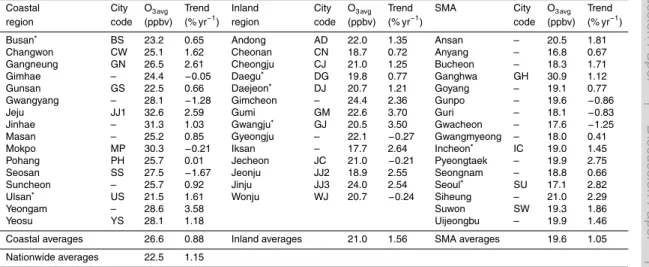
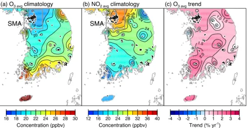
Climatological daily average O₃(O_{3 avg}) and its temporal linear trends are represented in Fig. 3 and Table 1 using data from 124 monitoring sites distributed nationwide in 46 cities for the past 12 yr period. The spatial map of climatological daily average NO2

5

(NO_{2 avg}) is also shown in Fig. 3. In Table 1, the cities are categorized into three geo-graphical groups: 16 coastal cities, 14 inland cities, and 16 cities in the Seoul Metropoli-tan Area (SMA). We separated the SMA cities from the other two groups since the SMA is the largest source region of anthropogenic O₃precursors in South Korea. The SMA occupies only 11.8 % (11 745 km2) of the national area, but has 49 % (25.4 million) of

10

the total population and 45 % (8.1 million) of total vehicles in South Korea. It is es-timated that approximately 27 % (291 kt) of total NO_x emissions and 34 % (297 kt) of the volatile organic compounds (VOCs) emissions in South Korea are from the SMA in 2010 (KMOE, 2013). Therefore, the climatological NO2 avgconcentration in the SMA is

much higher than that in other region (Fig. 3b).

15

In general, O3 concentrations are high at the coastal cities, low at the inland cities,

and lowest at the SMA cities in South Korea. Along with Table 1, Fig. 3a shows that the 12 yr average of O_{3 avg} is high at the southern coastal cities such as Jin-hae (31.3 ppbv), Mokpo (30.3 ppbv), and Yeosu (28.1 ppbv), with the highest value at Jeju (32.6 ppbv), and low at the inland metropolitan cities such as Daegu (19.8 ppbv),

20

Gwangju (20.5 ppbv), and Daejeon (20.7 ppbv), with lowest values at the SMA cities including Seoul (17.1 ppbv), Incheon (19.0 ppbv) and Anyang (16.8 ppbv).

Compared to the regional background concentration of 35–45 ppbv at five back-ground measurement sites around South Korea (KMOE, 2012), the averaged O₃ con-centrations in the SMA and inland metropolitans are much lower while those at the

25

(12)

ACPD

14, 1191–1238, 2014

J. Seo et al.

Title Page

Tables Figures

◭ ◮

Back Close

Full Screen / Esc

Discussion

P

a

per

|

D

iscussion

P

a

per

|

Discussion

P

a

per

|

Discuss

ion

P

a

per

|

higher NO_{2 avg}region. Substantial emissions of anthropogenic NO in the SMA and other inland metropolitans lead NOx titration effects even in the absence of photochemical

reactions during the night, and thus the averaged O3 concentrations are depressed

by 10–20 ppbv lower than the regional background concentration (Ghim and Chang, 2000). A recent modeling study by Jin et al. (2012) has suggested that the maximum

5

O3 concentrations in the SMA, especially in Seoul and Incheon, are VOCs-limited. In

the coastal region, on the other hand, low emissions of NO with dilution by the strong winds weaken the titration effect and result in the high O3concentrations. The dynamic

effect of land-sea breeze is another possible factor of the high O3levels at the coastal

cities. Oh et al. (2006) showed that a near-stagnant wind condition at the development

10

of sea breeze temporarily contains O₃ precursors carried by the o_ffshore land breeze during the night, and following photochemical reactions at mid-day produces O3. The

relationship between O3and wind speed and direction will be shown in Sects. 3.2 and

3.5 respectively.

In terms of temporal trends, the surface O3concentrations in South Korea have

gen-15

erally increased for the past 12 yr as shown in Fig. 3c and Table 1. The averaged tempo-ral linear trend of O_{3 avg}at 46 cities nationwide is₊1.15 % yr−1(₊0.26 ppbv yr−1), which is comparable with observed increasing trends of approximately+0.5–2 % yr−1in var-ious regions in the Northern Hemisphere (Vingarzan, 2004). Compared with prevvar-ious studies in East Asia, the overall increasing trend of O3 in South Korea is smaller than

20

recent increasing trends over China of+1.1 ppbv yr−1 in Beijing for 2001–2006 (Tang et al., 2009) and+0.58 ppbv yr−1in Hong Kong for 1994–2007 (Wang et al., 2009) but slightly larger than increasing trend over Japanese populated areas of+0.18 ppbv yr−1 for 1996–2005 (Chatani and Sudo, 2011).

Several factors that could influence the overall increase of O3 over East Asia were

25

(13)

ACPD

14, 1191–1238, 2014

J. Seo et al.

Title Page

Tables Figures

◭ ◮

Back Close

Full Screen / Esc

Discussion

P

a

per

|

D

iscussion

P

a

per

|

Discussion

P

a

per

|

Discuss

ion

P

a

per

|

suggested the long-term variations in meteorological fields as a possible important fac-tor although further studies are required. In particular, it is well known that insolation and temperature are important meteorological factors in O3variation. While insolation

directly affects O₃production through photochemical reactions, increased temperature affects net O3 production rather indirectly by increasing biogenic hydrocarbon

emis-5

sions, hydroxyl radical (OH) with more evaporation, and NOxand HOxradicals by

ther-mal decomposition of peroxyacetyl nitrate (PAN) reservoir (Sillman and Samson, 1995; Olszyna et al., 1997; Racherla and Adams, 2006; Dawson et al., 2007).

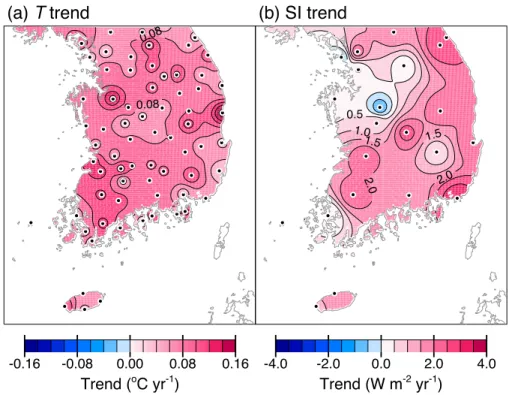
The O3 increasing trend in Fig. 3c is possibly affected by changes in

meteorologi-cal variables. Figure 4 shows temporal linear trends of daily average temperature (T)

10

and insolation (SI). Despite the spatial discrepancy between trends of O₃(Fig. 3c) and meteorological variables (Fig. 4), both temperature and insolation have generally in-creased in South Korea for the past 12 yr. The spatial mean of temporal linear trend in temperature at 72 weather stations nationwide is approximately₊0.09◦C yr−1, which is much higher than+0.03◦C yr−1for the Northern Hemispheric land surface air

tem-15

perature for 1979–2005 (IPCC, 2007). This high increasing trend of temperature in South Korea is probably due to urban heat island e_ffect with rapid urbanization. The averaged temporal linear trend of insolation at 22 weather stations nationwide is about

+1.47 W m−2yr−1 despite the decreasing phase of solar cycle during the 2000s. This is possibly caused by reduction in particulate matter emissions due to enhanced

envi-20

ronment regulation in South Korea during the recent decade (KMOE, 2012).

Although O3and related meteorological variables such as temperature and insolation

have recently increased in South Korea, the spatial patterns of their temporal trends do not show clear similarity. In addition, the spatial distribution of O3 trends is rather

inhomogeneous even on a metropolitan scale. For instance, Table 1 shows a wide

25

range of O₃trends among the SMA cities from−1.25 % yr−1of Gwacheon to₊2.82 %

yr−1of Seoul. The spatial inhomogeneity in O3trend and the trend differences among

O3, temperature, and insolation imply that the long-term O3 trends in South Korea

(14)

ACPD

14, 1191–1238, 2014

J. Seo et al.

Title Page

Tables Figures

◭ ◮

Back Close

Full Screen / Esc

Discussion

P

a

per

|

D

iscussion

P

a

per

|

Discussion

P

a

per

|

Discuss

ion

P

a

per

|

changes in local precursor emissions or transport of O₃ and its precursors. The local effects of precursor emission on the long-term changes in O3are further examined in

Sect 3.6.

3.2 Relationships between O3and meteorological variables

A multiple linear regression model is here adopted to explain relationships between

5

O_{3 8 h}and each of key meteorological variables such asTmax, SI, TD, PS, WS, and RH.

To exclude day-to-day short-term fluctuations or white noises from the original time-series, KZ29,3was applied to each variable before the regression process and yielded

baselines of each variable. As a result of the linear regression, squared correlation coefficients (R2) between O3 8 h and each meteorological variable were calculated for

10

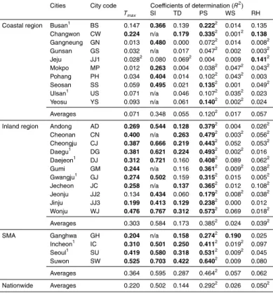
72 air quality monitoring sites distributed in 25 cities nationwide and summarized in Table 2. The nationwide average ofR2 is 0.50 for SI, 0.29 for PS, 0.22 for T_max, 0.14 for TD, 0.05 for RH, and 0.03 for WS, respectively. In South Korea, SI,Tmax, and TD

generally show positive correlations with O3 levels while PS is negatively correlated

with O₃ variations. Since the short-term variability in each variable is excluded, the

15

negative correlation between O₃ and PS is related to their seasonal cycle rather than continuously changing weather system of high and low. PS in South Korea located on the continental east coast is mostly affected by the cold continental high pressure air mass during the winter when the O₃concentrations are lowest. On the other hand, WS and RH show weak correlations with O3variations.

20

TheR2distributions forT_maxand SI are represented in Fig. 5. Figure 5a and b shows a common spatial pattern with high correlations at the inland and SMA cities and low correlations at the coastal cities. For instance, the averageR2 value with Tmax for the

coastal cities is only 0.07, which is much smaller than 0.36 for the SMA cities and 0.30 for the inland cities. Also, the average R2 values with SI are 0.60 for the SMA

25

cities and 0.58 for the inland cities, but 0.35 for the coastal cities. Despite the similar pattern between Fig. 5a and b, theR2values of SI are much higher than those ofTmax

(15)

ACPD

14, 1191–1238, 2014

J. Seo et al.

Title Page

Tables Figures

◭ ◮

Back Close

Full Screen / Esc

Discussion

P

a

per

|

D

iscussion

P

a

per

|

Discussion

P

a

per

|

Discuss

ion

P

a

per

|

influence of insolation on O₃levels by photochemical production (Dawson et al., 2007; and references therein). The apparent R2 differences among three regions indicate that temporal variations of O3at the SMA and inland cities are much more sensitive to

SI andTmax than those at the coastal cities. The low dependence of O3 on Tmax and

SI at the coastal cities means that the photochemical reactions of precursors are less

5

important for determining O3levels there compared to the SMA and inland cities.

The meteorological effects on O₃at the inland, coastal, and SMA cities are also ex-amined by daily minimum O3(O3 min). In the polluted urban area, the O3concentration

reaches near-zero minima during the night since O3 is reduced by NOx titration and

dry deposition in the absence of photochemical reactions. However, if O₃ is

persis-10

tently transported from the high-O3 background, the concentrations will keep higher

levels even at the nighttime (Ghim and Chang, 2000). Therefore, the high O3 min near

the coast (see Fig. 6a and Table 3) implies the large influences of the background O₃ transport at the coastal cities. Previous analyses of frequency distributions of O3

con-centrations have also shown that the O3levels at the coastal cities such as Gangneung,

15

Jeju, Mokpo, Seosan, and Yeosu are affected by the background O₃transport different from Seoul where the effect of local precursor emission is dominant (Ghim and Chang, 2000; Ghim, 2000).

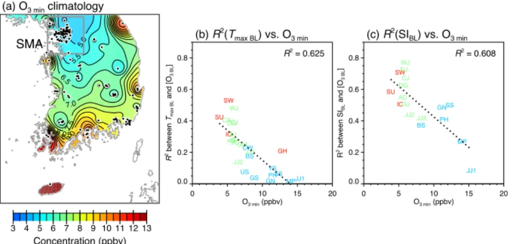
Compared to the spatial distribution of R2 between O₃ and T_max or SI in Fig. 5a and b, O3 min distribution in Fig. 6a shows high O3 min at the coastal cities where the

20

R2 is low and low O3 min at the inland cities where the R 2

is high. These opposite patterns suggest that the meteorological effects on the O₃ production and transport effects of background O3 are negatively correlated for the South Korean cities. The

clear negative correlations are also shown in scatter plots (Fig. 6b and c). In both two scatter plots, the three geographical groups of cities (blue for the coastal cities,

25

(16)

ACPD

14, 1191–1238, 2014

J. Seo et al.

Title Page

Tables Figures

◭ ◮

Back Close

Full Screen / Esc

Discussion

P

a

per

|

D

iscussion

P

a

per

|

Discussion

P

a

per

|

Discuss

ion

P

a

per

|

NO_x titration process despite the transport effects of background O₃. Among the SMA cities, on the other hand, Ganghwa (GH) has much higher O3 min compared to other

SMA cities. Ganghwa is a rural county located on the northwestern coast of the SMA. Therefore, both small NO_x emissions there and transport of regional background O₃ from the Yellow Sea affect the characteristics of O3in Ganghwa.

5

The different meteorological effects on O3 between the coastal and inland regions

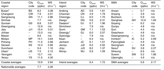
are further examined with wind speed. Daily average wind speed (WS) data over South Korea are averaged for 12 yr. The 12 yr averaged WS are summarized in Table 3 and presented in spatial map of Fig. 7a, which show high wind speed in the coastal region and low wind speed in the inland region. Figure 7b and c shows that the averaged

10

wind speeds of 25 cities are positively correlated with O_{3 min} and are negatively cor-related with theR2 between O3 and Tmax. In general, since the stronger wind speed

causes the less effective photochemical reaction due to the ventilation effect, the high wind speed with the high O3levels in the coastal region is attributable to the transport of

background O3. On the other hand, the weaker wind speed induces more effective

pho-15

tochemical reaction through the longer reaction time in stagnant condition as well as more enhanced aerodynamic resistance to dry deposition (Jacob and Winner, 2009). Therefore, the meteorological effects on the O3productions become more important in

the inland region where the wind speeds are lower.

3.3 Probability of O3exceedances related to temperature

20

Probability of O₃ exceeding air quality standard in a given range of temperature is useful to speculate about potential sensitivity of O3 concentration to climate change

(Lin et al., 2001; Jacob and Winner, 2009). We here calculated the probabilities of high O₃ occurrence that O_{3 8 h}exceeds the Korean air quality standard of 60 ppbv (KMOE, 2012) as a function of the daily maximum temperature (Tmax) for the coastal, inland,

25

and SMA cities. Similar to the analyses in Lin et al. (2001) for the contiguous United States, Fig. 8 shows that the probabilities of O3exceedances increase withTmaxat the

(17)

ACPD

14, 1191–1238, 2014

J. Seo et al.

Title Page

Tables Figures

◭ ◮

Back Close

Full Screen / Esc

Discussion

P

a

per

|

D

iscussion

P

a

per

|

Discussion

P

a

per

|

Discuss

ion

P

a

per

|

almost doubled by about 4◦C increase inTmaxand reach 27 % at 30 ◦

C. In the coastal region, on the other hand, the probability of O3 exceedance increases up to 12–13 %

withTmaxchange from 10 ◦

C to 20◦C and does not increase significantly forTmaxabove

20◦C. This is consistent with the spatial feature of the meteorological e_ffects on O₃ levels, which are high at the inland and SMA cities and low at the coastal cities as

5

described in the previous section. Therefore, the probability of high O3occurrence will

be more sensitive to the future climate change at the inland and SMA cities than at the coastal cities. In the previous modeling study by Boo et al. (2006),Tmaxover the Korean

peninsula is expected to rise by about 4–5◦C to the end of 21st century owing to the global warming. This indicates considerable future increases in exceedances of the O₃

10

air quality standard over South Korea except coastal regions.

3.4 Relative contributions of O3variations in different time-scales

Surface O3variation can be decomposed into short-term component ([O3 ST]), seasonal

component ([O_{3 SEASON}]), and long-term component ([O_{3 LT}]) by using the KZ-filter as described in Sect. 2.2. We evaluated relative contributions of each component to total

15

variance of original time-series. Overall, the relative contributions of [O3 LT] in Fig. 9c

are much smaller than those of [O_{3 ST}] in Fig. 9a and [O_{3 SEASON}] in Fig. 9b at all cities (Table 4). Therefore, sum of [O3 ST] and [O3 SEASON] account for the most of O3

varia-tions.

In Fig. 9a and b, the relative contributions of [O_{3 ST}] and [O_{3 SEASON}] show a strong

20

negative relationship spatially. The relative contributions of [O3 ST] are generally large

at the coastal cities (53.1 %) and small at the inland cities (45.9 %), whereas the rel-ative contributions of [O_{3 SEASON}] are small at the coastal cities (32.8 %) and large at the inland cities (41.9 %). Since [O3 ST] is related to synoptic-scale weather fluctuation

by transport of O3(Rao et al., 1995, 1997), the large relative contributions of [O3 ST] at

25

the coastal cities indicate the stronger effects of the synoptic-scale transport of back-ground O3there. On the other hand, [O3 SEASON] is driven mainly by the annual cycle of

(18)

ACPD

14, 1191–1238, 2014

J. Seo et al.

Title Page

Tables Figures

◭ ◮

Back Close

Full Screen / Esc

Discussion

P

a

per

|

D

iscussion

P

a

per

|

Discussion

P

a

per

|

Discuss

ion

P

a

per

|

contributions of [O_{3 SEASON}] at the inland cities are consistent with the higher impacts of temperature and insolation on the O3 therein (Figs. 5 and 9b). [O3 LT] explain less

than 10 % of the total variances, but its relative contribution is considerable in the south-western part of the Korean peninsula as displayed in Fig. 9c. This is related to relatively large long-term variability or trend in the region and is further discussed in Sect. 3.6.

5

3.5 Short-term variation of O3related to wind direction

The short-term components of O3([O3 ST]) account for a large fraction of total O3

vari-ation over South Korea. In Table 4, relative contributions of [O_{3 ST}] range from 32.7 % to 62.5 % and have a nationwide average of 49.8 %. Therefore, it is no wonder that high-O3episodes are mostly determined by day-to-day fluctuation of [O3 ST]. One

con-10

siderable factor influencing the short-term variation of O₃ is wind. Shin et al. (2012) displayed [O3 ST] on the wind speed-direction domain and showed that the effects of

episodic long-range transport and local precursor emission on the ambient O3

concen-trations could be qualitatively separated from [O_{3 ST}].

We here further investigate the transport effect on the short-term variations of O3

15

and the frequency of high-O3episodes using exp[O3 ST] and wind directions (WDs). As

described in Sect. 2.2, exp[O_{3 ST}] is a ratio of the raw O_{3 8 h}concentration to its baseline concentration in ppbv (exp[O_{3 BL}]). Thus, the O_{3 8 h} concentration is higher than the baseline O3 8 h concentration when exp[O3 ST]>1. We classified every single value of

exp[O3 ST] by 8 cardinal WDs during the high-O3season (May–October) at all available

20

monitoring sites within each city. The probabilities of exp[O_{3 ST}]>1 by each WD were compared with the probabilities exceeding the South Korean air quality standard of 60 ppbv for O3 8 h.

Figure 10 shows exp[O_{3 ST}] in the SMA cities (Seoul, Incheon, Suwon, and Ganghwa) with probabilities of exp[O3 ST]>1 and O3 8 h>60 ppbv for each WD. In Seoul,

high-25

O3 episodes are occurred most in northwesterly although westerly and northeasterly

(19)

ACPD

14, 1191–1238, 2014

J. Seo et al.

Title Page

Tables Figures

◭ ◮

Back Close

Full Screen / Esc

Discussion

P

a

per

|

D

iscussion

P

a

per

|

Discussion

P

a

per

|

Discuss

ion

P

a

per

|

SMA, where the predominant probability also appears in northwesterly wind in Incheon located in the west of Seoul (Fig. 10c and d), westerly wind in Suwon in the south of Seoul (Fig. 10e and f), and Ganghwa in the northwest of Seoul (Fig. 10g and h).

Sea–mountain breeze can explain the prevalence of high-O₃ episodes under west or northwesterly winds in the SMA. In the western coast of the SMA, there are many

5

thermoelectric power plants (see triangles in Figs. 11 and 12) and industrial complexes where directly emit a large amount of O₃precursors. Heavy inland and maritime trans-portation in those regions are also important source of NOx and hydrocarbon

emis-sions. Since the SMA is surrounded by the Yellow Sea in the west and mountainous region in the east (see Fig. 1), the westerly sea breeze are well developed under O₃

-10

conducive meteorological conditions such as high temperature and strong insolation with low wind speed (Ghim and Chang, 2000; Ghim et al., 2001). In addition, locally emitted precursors and transported background O3 from the west are trapped in the

SMA due to the westerly sea breeze and the mountainous terrain in the east of the SMA. Therefore, the O3concentrations in the SMA increase in such O3-conducive

me-15

teorological conditions with near-westerly winds.

Another factor to increase the high-O₃ probabilities in the near-westerly winds is long-range transport of O3 and its precursors from China. For example, Ghim

et al. (2001) reported some high-O3 cases in the SMA, which result from the

trans-port of O₃-rich air with strong westerly wind at dawn under overcast conditions. Oh

20

et al. (2010) also showed that the elevated layer of high O3 concentration over the

SMA is associated with the long-range transport of O3from eastern China. As the

mix-ing layer thickens over the SMA, the O₃concentration can increase by up to 25 % via vertical down-mixing process (Oh et al., 2010). Recently, Kim et al. (2012) showed that westerly winds also transport O3precursors such as NO2and carbon monoxide (CO)

25

from China to South Korea.

Interestingly, the high-O3 probability in Ganghwa (Fig. 10g and h) shows bimodal

(20)

ACPD

14, 1191–1238, 2014

J. Seo et al.

Title Page

Tables Figures

◭ ◮

Back Close

Full Screen / Esc

Discussion

P

a

per

|

D

iscussion

P

a

per

|

Discussion

P

a

per

|

Discuss

ion

P

a

per

|

county on the northwestern coast of the SMA, the double peak of high-O₃probability in easterly and westerly winds shows the effects of both local and long-range transport.

We extended the above exp[O3 ST] and WDs analysis to 25 cities over South

Ko-rea. The nationwide view of the high-O₃ probabilities is represented by the probabil-ities of exp[O3 ST] >1 and O3 8 h>60 ppbv by each wind direction during the high-O3

5

season (May–October). Figures 11 and 12 show spatial maps of the probabilities of exp[O_{3 ST}]>1 and O_{3 8 h}>60 ppbv, respectively. As indicators of major precursor emis-sion point source, we marked 26 of major thermoelectric power plants with triangles on the map. In general, the most of the thermoelectric power plants are located in the western coast of the SMA and southeastern coastal region of the Korean peninsula.

10

Thermoelectric power plants are important sources of NO_xin South Korea, accounting for 13 % (140 kt) of total NOx emission nationwide (KMOE, 2013). Considering that

in-dustrial complexes over South Korea are mostly concentrated near the power plants, the area with triangles in Figs. 11 and 12 represents major sources of O₃precursors.

In Figs. 11 and 12, the both probabilities of exp[O3 ST]>1 and O3 8 h>60 ppbv are

15

generally high on a national scale in the near-westerly wind conditions (Figs. 11f–h and 12f–h). The prevailing westerly wind of the synoptic-scale flow transports O₃ and its precursors from China to South Korea and thus increases the probability of high-O3 episodes as well as high O3 concentrations. However, on a local scale, the high

probability regions of high-O₃ correspond to downwind of the thermoelectric power

20

plants. For example, the high probabilities of high-O3in the southeastern part of South

Korea, downwind of power plants along the southeastern coast, also appear even in the easterly or southerly wind (Figs. 11c–e and 12c–e). Therefore, the spatial features of the high-O3 probabilities in each wind direction could be associated with both local

effect of precursor emission and long-range transport from the continent.

25

3.6 Long-term variation of O3and local precursor emissions

(21)

ACPD

14, 1191–1238, 2014

J. Seo et al.

Title Page

Tables Figures

◭ ◮

Back Close

Full Screen / Esc

Discussion

P

a

per

|

D

iscussion

P

a

per

|

Discussion

P

a

per

|

Discuss

ion

P

a

per

|

trend can be represented as a sum of the seasonal component ([O_{3 SEASON}]) and long-term component ([O3 LT]) trends. The spatial trend distributions of [O3 BL] and its two

separated components of seasonal and long-term components are shown in Fig. 13. It is noted that the period used in Fig. 13 is shorter than the total period of original data because of truncation effect in the KZ-filter process. The long-term component

5

obtained by the KZ-filter of KZ365,3 loses 546 days at the beginning and end of original

time-series.

The increasing trends of O3 are generally high in the SMA and southwestern part

and low in the southeastern coastal region of Korean peninsula (Fig. 13a). This spatial inhomogeneity of the O₃ trends over South Korea is mainly contributed by the

long-10

term component trends (Fig. 13c) rather than the seasonal component trend (Fig. 13b). Therefore, the large spatial variability in local precursor emissions induced the spatial inhomogeneity of O3trends in South Korea. On the other hand, relatively homogeneous

distribution of the seasonal component trends implies that meteorological influences on the long-term changes in O3have little regional dependence nationwide.

15

Since the spatially inhomogeneous O3trends are related to the local precursor

emis-sions, we also tried to investigate their relationship with NO₂ measurement data. To detect temporally synchronous and spatially coupled patterns between the long-term variations of O3and NO2, we applied the SVD to [O3 LT] and the long-term component

of NO₂([NO_{2 LT}]). [NO_{2 LT}] was simply obtained by applying the KZ-filter of KZ_365,3to the

20

log-transformed NO2 time-series. The SVD is usually applied to two combined

space-time data fields, based on the computation of a temporal cross-covariance matrix be-tween two data fields. The SVD identifies coupled spatial patterns and their temporal variations, with each pair of spatial patterns explaining a fraction of the square covari-ance between the two space-time data sets. The square covaricovari-ance fraction (SCF) is

25

largest in the first pair (mode) of the patterns, and each succeeding mode has a maxi-mum SCF that is unexplained by the previous modes.

The first three leading SVD modes (singular vectors) of the coupled O3 and NO2

(22)

ACPD

14, 1191–1238, 2014

J. Seo et al.

Title Page

Tables Figures

◭ ◮

Back Close

Full Screen / Esc

Discussion

P

a

per

|

D

iscussion

P

a

per

|

Discussion

P

a

per

|

Discuss

ion

P

a

per

|

second, and third modes are 63.7 %, 23.6 %, and 7.3 % respectively. Figure 14 dis-plays the expansion coefficients (coupled spatial patterns) and their time-series of the first mode along with spatial map of the [NO2 LT] trends. The dominant first mode of

the O3 and NO2 long-term components (Fig. 14a and b) is very similar to the spatial

distributions of [O_{3 LT}] trends (Fig. 13c) and [NO_{2 LT}] trends (Fig. 14c) respectively. In

5

Fig. 14d, the strong coherence in the time-series is observed between the first modes of the [O3 LT] and [NO2 LT] with a correlation coefficient of 0.98. The results of SVD

anal-ysis suggest that the long-term variations of O3 and NO2in South Korea have similar

temporal evolutions with di_fferent spatial patterns.

The differences in spatial patterns of [O3 LT] and [NO2 LT] as shown in Fig. 14a and

10

b are required to be further investigated. Since the VOCs emissions from industry, transportation, and the solvent usage in construction are large in South Korea (KMOE, 2013), further analyses of VOCs measurements are needed. On top of that, espe-cially in South Korea, biogenic precursor emissions are also potentially important for the analysis due to dense urban vegetation in and around metropolitan areas.

There-15

fore, there remains the limitation of current data analysis due to insufficient emission analyses and measurement data of the VOCs and NOxin South Korea.

4 Conclusions

This study investigated various spatio-temporal features and inter-relationship of sur-face O3and related meteorological variables over South Korea based on ground

mea-20

surements for the period 1999–2010. A general overview of surface O₃ in terms of spatial distributions and its temporal trend is provided based on its decomposed com-ponents by the KZ-filter.

In South Korea, the O₃ concentrations are low at the inland and SMA cities due to the NOxtitration by anthropogenic emissions and high at the coastal cities possibly due

25

to the dynamic effects of the sea breeze. The averaged O3levels in South Korea have

(23)

ACPD

14, 1191–1238, 2014

J. Seo et al.

Title Page

Tables Figures

◭ ◮

Back Close

Full Screen / Esc

Discussion

P

a

per

|

D

iscussion

P

a

per

|

Discussion

P

a

per

|

Discuss

ion

P

a

per

|

(+1.15 % yr−1). The recent increase of the O3 levels, which is common in the

North-ern Hemisphere and East Asia, may result from the recent increase of anthropogenic precursor emissions in East Asia and the long-term variations in meteorological e_ffects. We applied a linear regression model to investigate the relationships between O3

and meteorological variables such as temperature, insolation, dew-point temperature,

5

sea-level pressure, wind speed, and relative humidity. Spatial distribution of the R2

values shows high meteorological influences in the SMA and inland regions and low meteorological influences in the coastal region. The high meteorological influences in the SMA and inland regions are related to e_ffective photochemical activity, which results from large local precursor emissions and stagnant condition with low wind speeds. On

10

the other hand, the low meteorological influences in the coastal region are related to large transport e_ffects of the background O₃ and ventilation and dry deposition with high wind speeds.

In the SMA and inland region, the high-O3 probability (O3 8 h>60 ppbv) increases

with the daily maximum temperature rise. Specifically in the SMA, the most populated

15

area in South Korea, the probability of the O3exceedances is almost doubled for about

4◦C increase in daily maximum temperature and reached 27 % at 30◦C. It is noted that the variations in O₃exceedance probabilities according to the maximum tempera-ture show an approximate logarithmic increase in the SMA and inland regions. It thus implies that these regions will experience more frequent high-O3 events in the future

20

climate conditions with the increasing global temperature.

The O3 time-series observed at each monitoring site can be decomposed into the

short-term, seasonal, and long-term components by the KZ-filter. Relative contribu-tions of each separated component show that the short-term and seasonal variacontribu-tions account for most of the O3variability. Relative contributions of the short-term

compo-25

nent are large at the coastal cities due to influence of the background O3transport. In

(24)

ACPD

14, 1191–1238, 2014

J. Seo et al.

Title Page

Tables Figures

◭ ◮

Back Close

Full Screen / Esc

Discussion

P

a

per

|

D

iscussion

P

a

per

|

Discussion

P

a

per

|

Discuss

ion

P

a

per

|

The transport effects on the short-term component are shown in the probability dis-tributions of both high short-term component values and O3 exceedances for each

wind direction. During the high-O3 season (May–October) in South Korea, the

proba-bilities of both high short-term component O₃ and O₃ exceedances are higher in the near-westerly wind condition rather than in other wind directions. For the short-term

5

time-scale, the eastward long-range transport of O3 and precursors from China can

cause the nationwide high probabilities of O₃ exceedances in the near-westerly wind condition. However, the high probabilities of O3extreme events in downwind regions of

the thermoelectric power plants and industrial complexes are related to local transport of O₃precursors which apparently enhances the O₃levels.

10

The distribution of O₃ trends in South Korea is spatially inhomogeneous. Although the relative contributions of the long-term components are much smaller than those of other two components, such spatially inhomogeneous distribution of O3trend is mainly

contributed by the long-term component O₃trends rather than the seasonal component O3trend related to the long-term change of meteorological conditions. It is because the

15

long-term change of the local precursor emission has a localized effect on the long-term O₃ change. SVD between O₃ and NO₂shows that the long-term variations of O₃and NO2in South Korea have similar temporal evolutions with different spatial patterns. The

results of SVD analysis clearly demonstrate the influences of local precursor emissions on the long-term changes in O₃. However, the precise interpretation of the large

spa-20

tially inhomogeneous distribution in the long-term component O3trend is limited due to

lack of VOC measurements data.

The KZ-filter is a useful diagnostic tool to reveal the spatio-temporal features of O₃ and its relationship with meteorological variables. General features revealed by the KZ-filter analysis will provide a better understanding of spatial and temporal variations of

25

surface O₃ as well as possible influences of local emissions, transport, and climate change on O3 levels in South Korea. Our analyses would also be helpful as a

(25)

ACPD

14, 1191–1238, 2014

J. Seo et al.

Title Page

Tables Figures

◭ ◮

Back Close

Full Screen / Esc

Discussion

P

a

per

|

D

iscussion

P

a

per

|

Discussion

P

a

per

|

Discuss

ion

P

a

per

|

Acknowledgements. This study has been funded by the Green City Technology Flagship

Pro-gram of the Korea Institute of Science and Technology. Daeok Youn was supported by Chung-buk National University. Huikyo Lee performed this study as his private venture and is not in the author’s capacity as an employee of the Jet Propulsion Laboratory, California Institute of Technology.

5

References

Akimoto, H.: Global air quality and pollution, Science, 302, 1716–1719,

doi:10.1126/science.1092666, 2003.

Bell, M. L., Goldberg, R., Hogrefe, C., Kinney, P. L., Knowlton, K., Lynn, B., Rosenthal, J., Rosenzweig, C., and Patz., J. A.: Climate change, ambient ozone, and health in 50 US cities,

10

Climatic Change, 82, 61–76, doi:10.1007/s10584-006-9166-7, 2007.

Bernard, S. M., Samet, J. M., Grambsch, A., Ebi, K. L., and Romieu, I.: The potential impacts

of climate variability and change on air pollution-related health effects in the United States,

Environ. Health Persp., 109, 199–209, 2001.

Boo, K.-O., Kwon, W.-T., and Baek, H.-J.: Change of extreme events of temperature and

pre-15

cipitation over Korea using regional projection of future climate change, Geophys. Res. Lett., 33, L01701, doi:10.1029/2005GL023378, 2006.

Carmichael, G. R., Uno, I., Phadnis, M. J., Zhang, Y., and Sunwoo, Y.: Tropospheric ozone production and transport in the springtime in East Asia, J. Geophys. Res., 103, 10649– 10671, doi:10.1029/97JD03740, 1998.

20

Chatani, S. and Sudo, K.: Influences of the variation in inflow to East Asia on surface ozone over Japan during 1996–2005, Atmos. Chem. Phys., 11, 8745–8758, doi:10.5194/acp-11-8745-2011, 2011.

Dawson, J. P., Adams, P. J., and Pandis, S. N.: Sensitivity of ozone to summertime cli-mate in the eastern USA: A modeling case study, Atmos. Environ., 41, 1494–1511,

25

doi:10.1016/j.atmosenv.2006.10.033, 2007.