www.atmos-chem-phys.net/9/6055/2009/ © Author(s) 2009. This work is distributed under the Creative Commons Attribution 3.0 License.
Chemistry
and Physics
Evolution of stratospheric ozone and water vapour time series
studied with satellite measurements
A. Jones1, J. Urban1, D. P. Murtagh1, P. Eriksson1, S. Brohede1, C. Haley2, D. Degenstein3, A. Bourassa3, C. von Savigny4, T. Sonkaew4, A. Rozanov4, H. Bovensmann4, and J. Burrows4
1Department of Radio and Space Science, Chalmers University of Technology, Gothenburg, Sweden 2Department of Earth and Atmospheric Sciences, York University, Toronto, Canada
3University of Saskatchewan, Saskatoon, Canada
4Institute of Environmental Physics, University of Bremen, Germany
Received: 28 October 2008 – Published in Atmos. Chem. Phys. Discuss.: 14 January 2009 Revised: 29 June 2009 – Accepted: 15 July 2009 – Published: 20 August 2009
Abstract. The long term evolution of stratospheric ozone and water vapour has been investigated by extending satellite time series to April 2008. For ozone, we examine monthly average ozone values from various satellite data sets for nine latitude and altitude bins covering 60◦S to 60◦N and 20– 45 km and covering the time period of 1979–2008. Data are from the Stratospheric Aerosol and Gas Experiment (SAGE I+II), the HALogen Occultation Experiment (HALOE), the Solar BackscatterUltraViolet-2 (SBUV/2) instrument, the Sub-Millimetre Radiometer (SMR), the Optical Spectro-graph InfraRed Imager System (OSIRIS), and the SCanning Imaging Absorption spectroMeter for Atmospheric CHar-tograpY (SCIAMACHY). Monthly ozone anomalies are cal-culated by utilising a linear regression model, which also models the solar, quasi-biennial oscillation (QBO), and seasonal cycle contributions. Individual instrument ozone anomalies are combined producing an all instrument average. Assuming a turning point of 1997 and that the all instrument average is represented by good instrumental long term sta-bility, the largest statistically significant ozone declines (at two sigma) from 1979–1997 are seen at the mid-latitudes between 35 and 45 km, namely −7.2%±0.9%/decade in the Northern Hemisphere and−7.1%±0.9%/in the Southern Hemisphere. Furthermore, for the period 1997 to 2008 we find that the same locations show the largest ozone recovery (+1.4% and +0.8%/decade respectively) compared to other global regions, although the estimated trend model errors in-dicate that the trend estimates are not significantly different
Correspondence to:A. Jones ([email protected])
from a zero trend at the 2 sigma level. An all instrument av-erage is also constructed from water vapour anomalies dur-ing 1991-2008, usdur-ing the SAGE II, HALOE, SMR, and the Microwave Limb Sounder (Aura/MLS) measurements. We report that the decrease in water vapour values after 2001 slows down around 2004–2005 in the lower tropical strato-sphere (20–25 km) and has even shown signs of increasing until present. We show that a similar correlation is also seen with the temperature measured at 100 hPa during this same period.
1 Introduction
variation, such as atmospheric transport, temperature as well as climate change. Ozone depleting substance levels are thought to have reached their peak in between 1995 and 2000 in the upper stratosphere, but are not expected to return to pre 1980 values until 2050–2060, hence ozone’s recovery is equally as long (WMO, 2006). Recent estimations suggest that the Antarctic ozone hole will recover to pre 1980 values around 2068 (±10 years) (Newman et al., 2006).
Besides ozone, water vapour is of major interest. Not only is water vapour a dominant greenhouse gas in terms of its ra-diative properties, it is also a source of odd hydrogen that is important to ozone chemistry and hence ozone’s overall re-covery. It has been estimated that an increase in stratospheric water vapour by 1% per year could offset the ozone recovery by as much as 10–15 years (Dvortsov and Solomon 2001; Shindell 2001). Air is primarily transported to the lower stratosphere via the tropics as a result of deep convection, but the amount of water vapour entering is thought to be depen-dent on the temperature close to the tropical tropopause. Ad-ditionally, the increase of methane concentrations in the up-per stratosphere is an alternative pathway for increased wa-ter vapour concentrations in the upper stratosphere (SPARC, 2000).
More than 30 years of balloon sonde frost point hygrom-eter measurements at Boulder, Colorado (40◦N, 105◦W) show significant increases in water vapour of approximately 0.3–0.7% per year in the lower stratosphere between 1980 and 2001 (Scherer et al., 2008). A comparison made by Ran-del et al. (2004) using HALOE observations in an area near Boulder show the increase to be significantly less. As water vapour values are highly variable and combined with irreg-ular observations with typically a high level of uncertainty, it is difficult in many cases to distinguish trend features. A good example is the sudden decrease in lower stratospheric water vapour values in ∼2000–2001, which is thought to be connected to a combination of strong upwelling from the Pacific Ocean (Rosenhof et al., 2008) and an enhanced Brewer Dobson circulation that implies a lower local Tropo-spheric Tropopause Layer (TTL) temperature (Dohmse et al., 2008). As studies to date only present time series until 2005, we extend both stratospheric ozone and water vapour time series until April 2008 by using a combination of various satellite data sets. Many of these data sets have been used in previous studies, especially the historically longer and older times series such as from SAGE, HALOE, SBUV/2, and POAM III. Additionally, we also use shorter and newer time series from Odin/SMR (2001–present), Odin/OSIRIS (2001–present), Envisat/SCIAMACHY (2002–present), and Aura/MLS (2004–present). We analyse the long term evolu-tion of both species for measurements made between 60◦S and 60◦N and the altitude range of 20–45 km. The paper shows that even though a trend analysis is preferably made using the longer data sets, shorter data sets can be added to obtain a more reliable trend estimate, using a similar method to that of Steinbrecht et al. (2006).
2 Ozone and water vapour data sets
2.1 SAGE I+II
SAGE I and II in combination have produced one of the longest data sets of ozone, nitrogen dioxide, aerosols and wa-ter vapour. Although the combination of the two data sets is not contiguous, they provide the basis for making a robust trend analysis. SAGE I was launched on the Applications Explorer Mission-B satellite in February 1979 and ceased function in the early autumn of 1981, while SAGE II, which was part of the Earth Radiation Budget Satellite (Mauldin et al., 1985), launched in October 1984 and stopped measur-ing in October 2005. Both SAGE instruments utilised a solar occultation technique, comprising a multichannel sun pho-tometer observing in the Chappuis band centered at 600 nm for ozone and 940 nm for water vapour, measuring scattered solar light during sunrise and sunset throughout the 14 orbits per day (McCormick et al., 1989, 1992). Each satellite had a limited temporal and spatial coverage, tracking between typi-cally 60◦S and 60◦N and obtaining a global coverage within a month. Each derived profile for each measured species is of typically 1 km vertical resolution with an altitude uncer-tainty of ∼0.2–0.25 km from the surface to 70 km (Chu et al., 1989).
In this analysis we use SAGE I V7 (provided by L. Thoma-son, private communication, 2008) and SAGE II V6.2 data obtained from ftp://ftp-rab.larc.nasa.gov/pub/sage2/v6. 20. The SAGE II measurements of trace gases are highly susceptible to contamination of aerosol extinction and af-ter the Pinatubo eruption in June 1991 many measurements were corrupted by the high aerosol loadings, especially those below 25 km. Wang et al., have suggested filters that can be used in order to remove erroneous ozone measurements that are thought to be contaminated by aerosol (Wang et al., 2002). We use the same method by examining the observed amounts of aerosol found at each altitude and removing those that are believed to lead to erroneous ozone. Most of this con-tamination is present between 1991 and 1994. There are also similar problems with the water vapour product (Thomason et al., 2004). However, a report by Taha et al. (2004) suggests that there is no reliable filtering method using the aerosol extinction coefficients, hence we do not consider SAGE II water vapour data from 1984–1994, accounting for possible aerosol contamination, especially aerosol loading from the Pinatubo eruption in 1991. It should also be noted that from 1984-1991 SAGE II was the only satellite instrument mea-suring water vapour, hence there is no robust proof that the SAGE II data during this period is trustworthy. Finally, we also remove ozone and water vapour data that have a relative uncertainty greater than 50% so that only profiles of excellent precision are used.
while SAGE I precision is a factor of two worse than SAGE II (Cunnold et al., 1989). Systematic uncertainties of SAGE II are∼6% above 25 km where aerosol contamination is small and there is an extra 4% for where the aerosol contamination is large (<25 km) (Cunnold et al., 1989).
SAGE II has the longest water vapour data set to date (1984–2005). Validation of the V6.2 data set shows SAGE II profiles to agree with ATMOS/ATLAS-3 observations to within 15% with no obvious systematic bias between 12 and 40 km (Chiou et al., 2004). Another comparison shows agreement to within∼10% with POAM, ILAS, and HALOE, and 15–20% to MkIV at altitudes between 15 and 40 km (Taha et al., 2004).
2.2 SBUV/2
Another data set we use here is that of the Solar Backscatter Ultra-Violet SBUV/2 instrument. This data set is a combi-nation of two separate datasets, SBUV and SBUV/2 (collec-tively referred to as SBUV/2). The original SBUV instru-ment was aboard the NASA Nimbus-7 satellite launched in October 1978, while more improved versions of the SBUV/2 were developed and placed aboard subsequent missions, NOAA-9, December 1984, NOAA-11, September 1988, NOAA-14, December 1988, NOAA-16 September 2000, and NOAA-17 in June 2002. This nadir looking instrument mea-sures backscattered incoming solar radiation by using 12 different wavelengths, making both total ozone column and ozone profile estimates calculated from the ratio between the incoming spectral radiance and that of an observed backscat-tered signal (Bhartia et al., 1996). The data supplies only the average mean profile in a 5 degree latitude bin for each layer defined by the 15 pressure surfaces from 50–0.5 hPa from pole to pole. The vertical resolution of the version 8 data set is typically 6–8 km in the upper stratosphere and ap-proximately 6–10 km in the lowest stratosphere, which is an improvement compared to the previous versions thanks to an upgraded averaging kernel algorithm (Bhartia et al., 2004). This data set can be obtained from http://code916.gsfc.nasa. gov/Data services/merged/mod data.public.html. SBUV/2 data have recently been shown to have good consistency with SAGE II and HALOE data concerning time series analyses. However, it is stated that a high bias of ozone is present in the data above∼30 km after 2000 that will influence assess-ments of ozone recovery (Terao et al., 2007; WMO, 2006). SBUV/2 profile comparisons with HALOE V19 show a gen-eral agreement of 4–15% for pressure surface between 40 and 1.5 mb (Nazaryan et al., 2007)
Although, not originally intended, the SBUV/2 data are included here in this analysis. SBUV/2 V8 measurements are known to give a more positive trend after 2000 com-pared to other instrument data, especially in the upper strato-sphere (Terao et al., 2007). This effect is also seen earlier than 2000 in one such study where large significant SBUV/2 drifts of more than 5% are found compared to other time
series at various locations between 1992 and 1997 (Stein-brecht, 2006). However, the incorporation of SBUV/2 data is still important prior to this time, firstly because it gives a second reference to the merged SAGE time series up un-til the end of 1991 and secondly it also helps bridge the gap where the SAGE I data finishes and the SAGE II starts. The SBUV/2 data also confirm that there is no need to suspect that the SAGE I values are biased high and are in fact reason-able. A similar approach has been used in previous studies (Newchurch et al., 2003; Cunnold et al., 2004). We thus only use SBUV/2 data up until the end of 1991, when the HALOE time series begins. This way we firstly do not have to worry about SBUV/2’s long term effects of Pinatubo, and secondly, the final trend analysis will have contributions from two or more instruments at any one time, apart from the break pe-riod between the SAGE missions.
2.3 HALOE
The HALOE instrument aboard the Upper Atmosphere Research Satellite was operational from September 1991 to November 2005. Similarly to the SAGE instruments, HALOE was also a solar occultation instrument measuring many trace gases including ozone and water vapour. Ob-servations were made in the infrared part of the electromag-netic spectrum (between 2.45 and 10µm). (Russell et al., 1993). The HALOE occultation instrument was regarded highly sensitive and obtained 15 occultation measurements during each sunrise/sunset by comparing the solar spectra to the spectra obtained. This produced in essence a self calibrat-ing instrument with long term stability. The temporal cover-age was similar to that of the SAGE missions and the profile vertical resolution is approximately 2 km, making measure-ments between 10 and 50 km for ozone, while 10 to∼80 km for water vapour. Latitudinal coverage is from about 80◦N and 80◦S over the course of a year, while a global coverage is achieved in approximately six weeks. Data are ignored if the associated error on a profile is greater than 100%.
2.4 Odin/SMR
The Odin satellite was launched in the beginning of 2001 and is a joint initiative between Sweden, Canada, Finland and France. This small satellite comprises two instruments, the Sub-Millimeter Radiometer (SMR) and the Optical Spectro-graph InfraRed Imager System (OSIRIS). Both instruments are still operating at the time of writing. The Odin satellite is polar orbiting (82.5◦S to 82.5◦N) and is sun synchronous. The SMR instrument makes measurements of various species including stratospheric ozone and water vapour between 7 and 110 km by observing thermal emission in the microwave region during day and night (Murtagh et al., 2002; Frisk et al., 2003). SMR consists of five receivers, we use ozone from the 501.8 GHz band and the water vapour data product obtained from measurements around 488.9 GHz. We remove profiles if the quality flag is not equal to zero or a measure-ment response is less than 0.75
The newest version of SMR (level 2, produced at the Chalmers University of Technology, Sweden), v2.1 is anal-ysed for both stratospheric ozone and water vapour. Valida-tion of the ozone product shows a good agreement with var-ious other instruments presenting biases typically less than 10% in the stratosphere (Urban et al., 2005; Jones et al., 2007; Brohede et al., 2007; Jegou et al., 2008).
An overview of SMR water vapour observations is given by Urban et al. (2007). However, the latest v2.1 water vapour product has not yet been validated at this time. The vertical resolution for water vapour at 489 GHz line is 3–4 km be-tween∼20 and∼70 km while the ozone at 501.8 GHz has a typical vertical resolution of∼2.5 km between roughly 20 and 50 km.
2.5 Odin OSIRIS
As mentioned previously, the OSIRIS instrument is also on board the Odin satellite. The optical spectrograph is a grating spectrometer, which is used to produce atmospheric profiles of various atmospheric species including, O3, NO2, OClO, and aerosol by measuring limb scattered sunlight spectra in the visible region of 280–800 nm (Llewellyn et al., 2004). The vertical resolution of the latest ozone data product, v3.0, is ∼2 km in the middle stratosphere. This version shows good agreement with various other instruments using the same measurement technique (Haley et al., 2004), but also to the SMR instrument, helping to provide confidence in the robustness of the differing techniques (Brohede et al., 2007). Data filtering is also applied to the OSIRIS data where we remove data that are suspected to contain pointing problems, influences from the southern Atlantic anomaly, and from stray light associated with the moon. Similarly to the SMR data, we remove profiles if the quality flag is not equal to zero, if the one sigma measurement error is 100% larger than the corresponding measurement, or a measurement response less than 0.75.
2.6 SCIAMACHY
An instrument aboard the ENVISAT mission is the SCanning Imaging Absorption spectrometer for Atmospheric CHartog-raphY (SCIAMACHY). The instrument has the ability to ob-serve various atmospheric species, including ozone, in oc-cultation, limb scattering, and nadir viewing modes. In limb mode, thirty scans are made per profile from−3 to 92 km to obtain a vertical profile with a typical 4–4.5 km verti-cal resolution with full global coverage (Bovensmann et al., 1999). Here, we use the newest version 2.0 from the Insti-tute of Environmental Physics in Bremen (IUP), based on a simultaneous retrieval in the UV (Hartley-Huggins) and vis-ible Chappuis absorption bands of ozone. The algorithm is an extended version of the one described in von Savigny et al. (2005). The IUP Bremen provides the scientific products whereas the official offline data processor is run by ESA. As this data set is relatively new, there are no current reports of the performance of this version at the time of writing, hence we think that this analysis will help with the valida-tion process. The previous version 1.61 however has shown to have a low bias of typically 3–6% compared to SAGE II and lidar measurements between 16 and 40 km (Brinksma et al., 2006). This outcome is partly due to a known point-ing inaccuracy, which is accounted for in this newest ver-sion 2.0. Data can be obtained for SCIAMACHY ozone at http://www.iup.physik.uni-bremen.de/scia-arc.
2.7 MLS
Water vapour is also studied using the Microwave Limb Sounder (MLS) which was launched in August 2004 on the NASA Aura satellite. This is the second MLS instru-ment, whereas the previous instruinstru-ment, on board the Up-per Atmosphere Research Satellite (UARS and hence was named UARS MLS), operated for ∼8 years between 1991 and 1999, although the water radiometer ceased operation in 1993, hence this data is not included in the analysis. MLS is a limb scanning instrument, observing thermal emission at millimeter and sub-millimeter wavelengths (Waters et al., 2006). Similar to the Odin/SMR instrument, MLS has the ability to measure at night and is not affected by stratospheric clouds. The Aura satellite maintains a suborbital track cov-ering 82◦S to 82◦N. For MLS V2.2 data, water vapour has
1984 1989 1994 1999 2004 2
2.5 3 3.5 4 4.5 5
year 20−25 km
1984 1989 1994 1999 2004 5
6 7 8 9 10
25−35 km
1984 1989 1994 1999 2004 5
5.5 6 6.5 7 7.5 8
30S−30N, 35−45 km
1984 1989 1994 1999 2004 2
2.5 3 3.5 4 4.5 5
year 20−25 km
1984 1989 1994 1999 2004 5
6 7 8 9 10
25−35 km
1984 1989 1994 1999 2004 5
5.5 6 6.5 7 7.5 8
30N−60N, 35−45 km
1984 1989 1994 1999 2004 2
2.5 3 3.5 4 4.5 5
year
VMR [ppmv]
20−25 km
1984 1989 1994 1999 2004 5
6 7 8 9 10
VMR [ppmv]
25−35 km
1984 1989 1994 1999 2004 5
5.5 6 6.5 7 7.5 8
VMR [ppmv]
60S−30S, 35−45 km
A B C
D
E
F
G H I
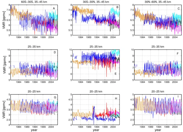
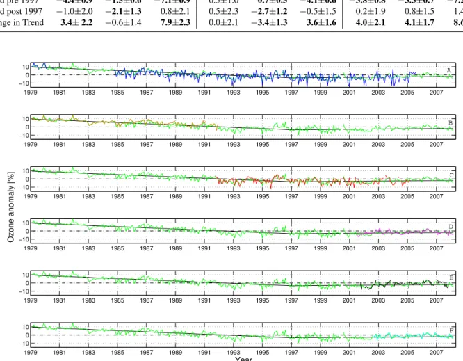
Fig. 1. Monthly mean ozone time series comparison of 6 instruments in nine altitude/latitude bins; SAGE I+II (blue), SBUV/2 (orange),
HALOE (red), SMR (magenta), OSIRIS (black), SCIAMACHY (cyan). The bins range from 60◦S to 60◦N in an altitude range from 20–45 km.
a good agreement to within 10% of these instruments for stratospheric measurements.
3 Methodology
3.1 Monthly mean comparisons
Although not the main objective in this paper, we show for both stratospheric ozone and water vapour how each individ-ual data set compares. As the trend analysis will focus on three altitude zones, 20–25 km, 25–35 km, and 35–45 km in three latitude bands (60◦S–30◦S, 30◦S–30◦N, and 30◦N– 60◦N) we show how monthly mean VMR values for each
instrument compare in these zones. This technique does not follow the conventional comparison method of profile to pro-file comparisons, but rather compares time series of average measurements over a long period of time as they are used in this analysis. Mismatches are thus possible in terms of time and space, but as each data set comprises a large number of measurements the stochastic error should be minimised when measurements are averaged. We have chosen these altitude ranges firstly because the first signs of ozone recovery are expected to be seen in the upper stratosphere (Jucks et al.,
1984 1989 1994 1999 2004 4
5 6 7
year
20−25 km 19844 1989 1994 1999 2004
5 6 7
25−35 km 19844 1989 1994 1999 2004
5 6 7 8
30S−30N, 35−45 km
1984 1989 1994 1999 2004 4
5 6 7
year
20−25 km 19844 1989 1994 1999 2004
5 6 7
25−35 km 19844 1989 1994 1999 2004
5 6 7 8
30N−60N, 35−45 km
1984 1989 1994 1999 2004 4
5 6 7
year
VMR [ppmv]
20−25 km 19844 1989 1994 1999 2004
5 6 7
VMR [ppmv]
25−35 km 19844 1989 1994 1999 2004
5 6 7 8
VMR [ppmv]
60S−30S, 35−45 km
A B C
D E F
G H I
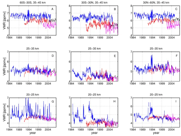
Fig. 2. Monthly mean water vapour time series comparison of 5 instruments in nine altitude/latitude bins; SAGE II (blue), HALOE (red),
SMR (magenta), and MLS (black). The bins range from 60◦S to 60◦N in an altitude range from 20–45 km.
Figures 1 and 2 illustrate each individual instrument monthly mean time series in each altitude/geolocation bin for ozone and water vapour, respectively. In both figures one can see clearly the seasonal cycles of both species, especially for ozone. The peaks and troughs seen here are not necessar-ily during the same month in each altitude/latitude bin due to the varying magnitudes of complex dynamical and chem-ical processes. The general circulation in the stratosphere is governed by the Brewer-Dobson circulation, which exists due to contrasts in differential heating between the equator and poles and is driven by wave motions in the extra-tropical stratosphere. Moreover, the magnitude of these wave per-turbations varies on an annual basis, producing differences in the interannual variability. Main sources for this varia-tion are from the Quasi-Biennial Oscillavaria-tion (QBO), annual oscillation (AO), and semi annual oscillation (SAO). For ex-ample, the QBO is a reversal of the regular west-east winds in the tropical stratosphere occurring approximately every 26 to 30 months (Baldwin et al., 2001). This ultimately varies the propagation speeds of the extra-tropical waves and hence the strength of the Brewer-Dobson circulation. During the late winter months, when the Brewer-Dobson circulation is at its strongest, air from the tropics is transported towards
the winter pole, accounting for the large ozone and water vapour concentration increments in the middle and lower stratosphere. In the upper stratosphere, ozone concentrations are also strongly influenced by the seasonal variation of solar UV intensity, where during the late summer months ozone maxima occur due to an enhanced photochemical production (Brasseur and Solomon, 2002).
we have filtered data for aerosol artifacts, large values appear to persist in the SAGE II data in the 20–25 km tropics bin (panel H). As a precaution we remove SAGE II data between 1991 and 1994 in this bin so as to remove the artifacts.
Most recent work involving satellite water vapour long term evolution use HALOE observations as the primary data set, while SAGE II data must be used with precaution due to aerosol contamination (Thomson et al., 2004). Although we remove SAGE II water vapour measurements from 1984– 1994 when examining the water vapour anomalies, we in-clude these years here in Fig. 2 just for illustration. It is clearly seen that SAGE II data are strongly contaminated during 1991 and 1994 in all bins. Figure 2 also shows that in the lower and middle stratosphere there is a reason-ably good agreement to within 0.5 ppmv between SAGE II, HALOE, MLS and SMR after 2000 in the middle and lower stratospheric bins (panels D–I). There are discrepan-cies at the higher stratospheric altitudes where larger bi-ases are seen (panels A–C). In all three latitude bins, SMR values are systematically lower than the other instruments (∼0.5 ppmv compared to HALOE), while SAGE II is sys-tematically larger (∼0.5 ppmv compared to HALOE). There is also a generally good agreement between HALOE, and MLS during overlapping time periods. The lowest altitude range shows SAGE II to be noisy and occasionally giving large mean monthly values after the Pinatubo eruption in 1991 (panel F–I) (Also seen in the ozone data in panel H in Fig. 1).
In summary, we have established that the monthly means from each instrument are generally consistent with each other and that biases are typically within 10% during overlapping periods.
3.2 Calculating ozone anomalies
The variations that we see in each individual time series are cyclic in nature and are associated mainly to seasonal (in-cluding SAO), QBO and solar cycles. Hence, by being able to separate the relative contributions of each of these pro-cesses we will be left with the unexplained variability of the monthly mean signal.
We follow a similar approach to that of Newchurch et al. (2003), and Steinbrecht et al. (2004, 2006) where monthly ozone anomalies are calculated by firstly removing the an-nual cycle. This is simply done for each instrument by find-ing the difference between each monthly mean value from their corresponding average (climatological) annual cycle. For example, the SAGE I+II mean January value calculated for all Januarys during 1979–2005 is subtracted from each individual SAGE I+II January VMR value.
The anomalies obtained here still have fluctuations associ-ated with the QBO and solar cycles. To remove these cycles we can model the ozone anomalies as a sum of terms incor-porating a linear trend and variations related to the QBO and solar cycles,
y(t )=at+b+
nQBO
P
i=1
cicos
2π t PQBO(i)
+disin
2π t PQBO(i)
+
nSolar
P
i=1
eicos
2π t
PSolar(i)
+fisin
2π t
PSolar(i)
+
N (t )
(1)
wherey(t )are the monthly ozone anomalies,t=1, 2, 3 . . .
nfor each individual data set. The first two components of Eq. (1) are the linear trend, where “a” is the magnitude of the trend and “b” is a constant att=0. On the second line is the quasi biennial component that employs a combination of sines and cosines. Similarly, the solar cycle is dealt with in the same way and is given on line three. TheN (t )term on the fourth line presents the noise residual term, or first order autocorrelation noise term, such that N (t )=φN (t )t−1+εt, whereεt is the white noise with mean zero and a common standard deviationσN. The unknowns in the modela,b,c,
d,e, andf, hence need to be determined in order to calculate the summed contributions for both the QBO and solar cycles. It should be noted that there is no need to include the seasonal cycle term as it has already been removed when calculating the ozone anomalies. Our main motivation for doing this was that we wanted to examine the anomalies before and after the removal of the smaller seasonal, QBO and solar terms for the sake of completeness.
We next produce ozone anomalies by subtracting the QBO and solar contributions from the deseasonalised anomalies. We then combine each individual deseasonalised anomaly time series to produce an all instrument average. To align individual anomaly time series that overlap in time, we cor-rect for the offsets. An important factor is that each individ-ual data set must overlap with at least one other data set for this method to work of with an overlap period of typically (at least) a couple of years, which is possible with the data sets we have chosen.
Lastly, for ozone we also estimate trends in each lati-tude/altitude bin, adopting the method from Appendix A in Reinsel et al. (2002). The assumption used in this method is that if there is a change in trend, the trend line itself is both linear and continuous. For this analysis we assume the turn around or break point year in the ozone trend occurs in January 1997, which is consistent with assumptions made in earlier studies (Steinbrecht et al., 2006; WMO, 2006; Newchurch et al., 2003; Cunnold et al., 2004).
3.3 QBO, SAO, and solar cycle contributions
1979 1981 1983 1985 1987 1989 1991 1993 1995 1997 1999 2001 2003 2005 2007 −5
0 5
ozone anomaly [%]
1979 1981 1983 1985 1987 1989 1991 1993 1995 1997 1999 2001 2003 2005 2007 −5
0 5
ozone anomaly [%]
1979 1981 1983 1985 1987 1989 1991 1993 1995 1997 1999 2001 2003 2005 2007 1000
1500 2000
Solar Flux [10
23 W/(m 2 Hz)]
1979 1981 1983 1985 1987 1989 1991 1993 1995 1997 1999 2001 2003 2005 2007 −20
0 20
year
Singapore Winds [ms−1]
A
B
C
D
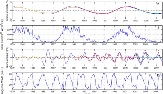
Fig. 3.Fitted QBO and solar components (AandCrespectively) of six instruments at 35–45 km, 30◦N–60◦N. SAGE I+II (blue), SBUV/2
(orange), HALOE (red), SMR (magenta), OSIRIS (black), SCIAMACHY (cyan). These estimates are based on harmonic oscillations fitted to each individual ozone time series. Also shown in(B)and(D)are the 10.7-cm solar flux and Singapore winds at 10 hPa respectively, for comparison.
compared to the Singapore winds proxy. We look at each in-dividual time series separately to determine which periods to use. In order to calculate the periods of thePQBOwe have used a simple Fast Fourier Transform (FFT) model that iden-tifies the possible harmonics needed to make a fit. We find in most cases that periods are between 7–9 and 15–32 months, which agrees with other previous studies (Newchurch et al., 2003; Steinbrecht et al., 2004, 2006; Cunnold et al., 2004), while 12 months is not included as it is accounted for when removing the seasonal cycle.
A similar method is applied to the 11 year solar cycle where more than one harmonic may be needed in order to fit the solar cycle, corresponding approximately to a proxy time series such as the 10.7-cm solar radio flux. We have tried various harmonic fits using both the FFT model and those de-scribed in earlier studies and have concluded that the best fits were periods of 63 and 127 months. These coupled harmon-ics are proven to show better fits compared to other models using more than two harmonics (Cunnold et al., 2004) and are hence used here commonly for all instruments.
For shorter data sets, such as HALOE, SMR, OSIRIS, MLS, and SCIAMACHY one may not be able to fit harmon-ics directly. This is less of a problem for the QBO, where periods are much shorter than the length of each these time series, but more significant problems are presented for longer oscillation periods, such as those associated with the solar cycle. As mentioned, the typical solar cycle period is every 11 years (or 132 months), much longer than any of the data sets mentioned above. To get around this problem we use the SAGE data as a proxy in order to fit both solar and QBO
cy-cles. This is simply done by extending one of the shorter time series prior to its start date using the SAGE data extending to time,t0(02/1979 for ozone, 10/1984 for water vapour). By using the extended time series we can identify harmonics by using the FFT model so that a fit can be made to the shorter time series. However, from this fit we only consider the os-cillations post the start date of the shorter time series, hence the SAGE data acts merely as a “dummy” time series.
1992 1994 1996 1998 2000 2002 2004 2006 2008 −5
0 5
ozone anomoly [%]
1992 1994 1996 1998 2000 2002 2004 2006 2008
−20 −10 0 10
Singapore Winds [ms−1]
Year
A
B
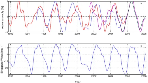
Fig. 4.Fitted QBO(A)of four instruments at 30◦S–30◦N, 25–35 km. SAGE II (blue), HALOE (red), SMR (magenta), and MLS (black).
These estimates are based on harmonic oscillations fitted to each individual water vapour time series. Also shown in(B)is the Singapore winds at 30 hPa shown for relative comparison.
The QBO contribution, shown in Fig. 3, panel C, produces a typical peak to peak amplitude of∼5–6%. For comparison, the Singapore winds proxy at 10 hPa are shown in panel D for comparison. Ozone values reach a maximum in between Jan-uary and FebrJan-uary in the Northern Hemisphere as a result of the stronger planetary wave activity, but during phases when the QBO winds become westerly (positive winds) ozone val-ues are less, which can be seen here for several years us-ing the SAGE and HALOE anomalies (1992, 1994, 1996, 1998/9, 2001, 2002/3, 2004/5, and 2007). The QBO effect on the water vapour anomalies for 30◦S–30◦N and 25–35 km is
shown in Fig. 4. Here, there is a better correlation in terms of shape and phase between the anomaly peaks and sinks and the QBO wind proxy. The difference in maxima and minima is typically 8–10%. We see a good phase fit in the tropics as there is typically no time lag since the QBO is a tropical phenomenon.
4 Results
4.1 Ozone trend analysis
Figure 5 illustrates an example of each individual instrument and their contribution to the all instrument average for the northern mid-latitudes (30◦N–60◦N, 35–45 km). The trend
line (black line) is calculated from the all instrument aver-age time series (green line). Also illustrated in panels A– F are the anomalies (i.e. deseasonalised and with contribu-tions of the QBO and solar cycles removed) from each in-strument overlaid in bold. We can see that there is a clear decrease in ozone values from 1979 until 1997 as indicated by the all instrument average (−7.2%/decade). The
instru-ments that contribute during this time, SAGE I+II, SBUV/2, and HALOE show consistency with each other during over-lapping periods, although the SBUV/2 anomalies are slightly larger than anomalies calculated for the whole SAGE I pe-riod, and for SAGE II during 1988–1991. The trend line af-ter 1997 indicates a slowing down of ozone depletion and that there is even an increase (1.4%/decade±2.3%, i.e. not statistically significant at the 95% confidence level). It can be seen visibly from 2001 that HALOE, SMR, OSIRIS, and SCIAMACHY all show a slight increase in ozone in this bin if one just considers the respective anomalies.
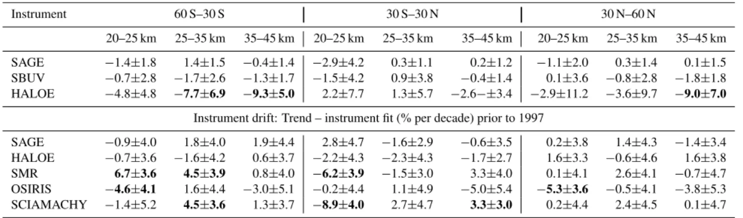
Table 1.Estimated trend values for the all instrument average before and after 1997. Also shown are the change in trend values. Plus minus values are the modeled uncertainties. Bold values are statistically significant at the 2 sigma level (95% confidence level).
60 S–30 S 30 S–30 N 30 N–60 N
20–25 km 25–35 km 35–45 km 20–25 km 25–35 km 35–45 km 20–25 km 25–35 km 35–45 km
Trend pre 1997 −4.4±0.9 −1.5±0.6 −7.1±0.9 0.5±1.0 0.7±0.5 −4.1±0.6 −3.8±0.8 −3.3±0.7 −7.2±0.9
Trend post 1997 −1.0±2.0 −2.1±1.3 0.8±2.1 0.5±2.3 −2.7±1.2 −0.5±1.5 0.2±1.9 0.8±1.5 1.4±2.3 Change in Trend 3.4±2.2 −0.6±1.4 7.9±2.3 0.0±2.1 −3.4±1.3 3.6±1.6 4.0±2.1 4.1±1.7 8.6±2.5
1979 1981 1983 1985 1987 1989 1991 1993 1995 1997 1999 2001 2003 2005 2007 −10
0 10
1979 1981 1983 1985 1987 1989 1991 1993 1995 1997 1999 2001 2003 2005 2007 −10
0 10
1979 1981 1983 1985 1987 1989 1991 1993 1995 1997 1999 2001 2003 2005 2007 −10
0 10
1979 1981 1983 1985 1987 1989 1991 1993 1995 1997 1999 2001 2003 2005 2007 −10
0 10
Ozone anomaly [%]
1979 1981 1983 1985 1987 1989 1991 1993 1995 1997 1999 2001 2003 2005 2007 −10
0 10
1979 1981 1983 1985 1987 1989 1991 1993 1995 1997 1999 2001 2003 2005 2007 −10
0 10
Year
A
B
C
D
E
F
Fig. 5.Ozone anomalies for six instruments for the 30◦N–60◦N and 35–45 km bin. Shown are the SAGE I+II (blue,A), SBUV/2 (orange,
B), HALOE (red,C), SMR (magenta,D), OSIRIS (black,E), and SCIAMACHY (cian,F). Also shown under-laid is the all instrument average (green). The vertical black line at 1997 indicates the estimated turn around date. Thin black line indicates the best fit trend to the all instrument average before and after 1997.
between hemispheres. The largest hemispheric difference is seen between 25–35 km, where the Southern Hemisphere shows a smaller trend (−1.5%/decade ±0.6%) compared to the Northern Hemisphere (−3.3%/decade ±0.7%). Al-though not shown here, we find this difference to be caused by the SBUV/2 anomalies. Firstly, considering SAGE alone, we find that the trends in these two bins are of similar magnitude (−3.6±1.2%/decade in Northern Hemisphere and
−3.0±1.4%/decade in the Southern Hemisphere). However, SBUV/2 anomalies are more negative in the Northern Hemi-sphere than the SAGE anomalies giving an overall more neg-ative trend for the all instrument average. The opposite is true for the Southern Hemisphere, such that SBUV/2 shows more
positive anomalies in comparison to SAGE, hence a less neg-ative trend is obtained. This result agrees with similar find-ings summarised in the WMO report (2006).
Table 2.A summary of the instrumental drifts of the six analysed instruments for the nine latitude/altitude bins before and after the break date in 1997. Plus minus values are the two standard deviation uncertainties, where bold values are statistically significant from zero. Drift is defined as the difference between each individual instrument time series and the all instrument average.
Instrument 60 S–30 S 30 S–30 N 30 N–60 N
20–25 km 25–35 km 35–45 km 20–25 km 25–35 km 35–45 km 20–25 km 25–35 km 35–45 km
SAGE −1.4±1.8 1.4±1.5 −0.4±1.4 −2.9±4.2 0.3±1.1 0.2±1.2 −1.1±2.0 0.3±1.4 0.1±1.5 SBUV −0.7±2.8 −1.7±2.6 −1.3±1.7 −1.5±4.2 0.9±3.8 −0.4±1.4 0.1±3.6 −0.8±2.8 −1.8±1.8 HALOE −4.8±4.8 −7.7±6.9 −9.3±5.0 2.2±7.7 1.3±5.7 −2.6−±3.4 −2.9±11.2 −3.6±9.7 −9.0±7.0
Instrument drift: Trend – instrument fit (% per decade) prior to 1997
SAGE −0.9±4.0 1.8±4.0 1.9±4.4 2.8±4.7 −1.6±2.9 −0.6±3.5 0.2±3.8 1.4±4.3 −1.4±3.4 HALOE −0.7±3.6 −1.6±4.2 0.6±3.7 −2.2±4.3 −2.3±4.3 −1.7±2.7 1.6±3.3 −0.6±4.6 1.6±3.8 SMR 6.7±3.6 4.5±3.9 0.8±4.0 −6.2±3.9 −1.5±3.0 3.3±4.0 0.1±4.1 2.6±4.1 −0.7±4.7 OSIRIS −4.6±4.1 1.6±4.4 −3.0±5.1 −0.2±4.4 1.1±4.9 −5.0±5.4 −5.3±3.6 −0.5±4.1 −3.8±5.3 SCIAMACHY −1.4±5.2 4.5±3.6 1.3±3.7 −8.9±4.0 2.7±4.7 3.3±3.0 0.2±4.4 2.4±4.5 0.1±4.7
Instrument drift: Trend – instrument fit (% per decade) after 1997
the southern mid-latitudes in this altitude region although the trend value is not significant at the two sigma level (0.8%/decade±2.1%) and is approximately a quarter of that calculated by Steinbrecht et al. (3.35%/decade±2.88%). We also calculate that the northern mid-latitudes between 35 and 45 km show a statistically non significant (at two sigma) in-crease of ozone anomalies (1.4%/decade±2.3%), which is less than the estimates reported by Steinbrecht et al. (∼−2.5 to 0.9%/decade ). Both northern and southern hemispheric 35–45 km bins show the largest significant change in trend (8.6%±2.5%/decade and 7.9%±2.3%/decade, respectively). In the tropical upper stratosphere our trends are more neg-ative compared to those found by Steinbrecht et al. (2006) (1.94%/decade±1.89%), while our trend estimate is not sig-nificant (−0.5%/decade ±1.5%). As current ozone levels are typically 10–12% lower than pre 1980 values in the up-per extra-tropical stratosphere, it would take approximately another 70 years to reach pre 1980 values if ozone were to increase linearly at a rate of 1.4%/decade. This would be the mid to late 21st century, which is later than the near linear model estimates of 2040–2050 presented by the WMO (2006). However, there is still too much uncertainty in the calculated post 1997 trend for it to be statistically sig-nificant from a zero trend with a 95% confidence.
4.2 Drift and calibration issues
An important consideration is that of instrument calibration and long term drift, which may influence the trend value. Ta-ble 2 presents a summary of instrumental drift defined as the difference between the trend value derived from the all in-strument mean for each latitude/altitude bin and the individ-ual fit from the independent instrumental anomalies (given as percent per decade) within the corresponding bins. The error
bars in Table 2 are the 2 sigma uncertainties (95% confidence interval) calculated from equations suggested by Reinsel et al. (2003). Drifts that are considered statistically significant are given in bold.
It has been suggested that VMR measurements made on a pressure grid surface, such as SBUV/2 may produce less negative trends compared to instruments measuring density profiles on a geometric grid (HALOE and SAGE). If a tem-perature trend persists then it implies that air densities on these pressure surfaces will also vary over time. Moreover, the pressure surfaces themselves will move vertically. For example, pressure surfaces are moving vertically downwards in a cooling stratosphere (Ramaswamy et al., 2001). Ulti-mately, a less negative ozone trend is expected when using a pressure grid, hence SBUV/2 ozone anomalies values are less negative, most notably at higher stratospheric altitudes (WMO, 2006) as seen in Table 2. However, there are no cases where the SBUV/2 anomalies are statistically signifi-cant at the 2 sigma level. We also note that there appear to be no apparent SBUV/2 drifts below the ozone maximum in all bins, where earlier analyses had issued a warning that using SBUV/2 V8 measurements may give unreliable information on the vertical distribution of ozone (Terao et al., 2007).
peaking EESC levels) compared to 1979–1991 ozone de-clines, which explains the HALOE anomaly fits being less negative than the respective 1979–1997 trend values for each bin, especially those concerning the higher altitude, extra-tropical bins.
A large difference in long term drift between SAGE II and the other instruments is seen after 1997 in the 30◦S– 30◦N, 20–25 km bin, where SAGE II exhibits a more nega-tive trend compared to the other instruments. The calculated trend line from 1979 to 1997 illustrated in Table 1 shows an increase in ozone values (0.5%/decade +/−1.0%), while after 1997 values continue to increase at the same rate (0.5 +/−2.3%/decade). We find SAGE values to thus be more negative between 2002 and 2005 compared to the other over-lapping instruments. Although the SAGE drift is not signifi-cant the fact that its anomalies show this tendency, probably means that the measurements should not be totally trusted.
There are also random occasions where the shorter time series instruments give significant long term drifts. Five of eight cases are found in the lowest altitude bins, possibly ow-ing to differences in spatial samplow-ing, as result of flagged or filtered data. The other two significant cases are both found in the southern mid-latitudes, 25–35 km (SMR and SCIAMACHY). Both of these instruments show more neg-ative anomalies than the corresponding trend, as do two of the other three instruments in the bin (SAGE and OSIRIS, which exhibit non significant drift). This implies that al-though SMR and SCIAMACHY are albeit significantly more negative than the trend value, they are at least in agreement with the majority of the other instruments in the bin.
The other drifts in Table 2 are not statistically significant at the 2σlevel hence the associated anomalies give confidence in the all instrument mean ozone time series for all bins. 4.3 Turn around year
Another important factor to account for is if and where a turn around in a trend is believed to be present. It has been sug-gested that a turn around point for ozone occurred sometime between 1995 and 1999 as a result of recorded declines of HCl and HF concentrations (Waugh et al., 2001; Newchurch et al., 2003; WMO, 2006). It is most likely that we will see a turn around firstly in the upper stratosphere as it is here where halocarbons are photochemically broken down due to strong UV light (Jucks et al., 1996). Eventually in time, a turn around point in the lower stratosphere should become apparent as the halogen gases are slowly phased out.
In this analysis we have first assumed a turn around date of 1997 to be constant for each individual bin. This is done as we want to be consistent with previous analyses that also use the 1997 fixed turn around date for all altitude and lati-tude regions. This particular date is thought to be the near-est whole year when equivalent effective stratospheric chlo-rine (EESC) reached its peak before its slow decline in the extra-tropical lower-middle stratosphere based on a 3 year
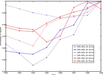
time lag of mean aged air (Newman et al., 2007). However, an assumption that 1997 is the turn around time for all lat-itudes and altlat-itudes could be considered as somewhat crude as the dynamics and chemistry involved vary with time and space, implying that the turn around time may differ. By moving the turn around year by just one year or even a few months can give vast differences in trend magnitude both be-fore and after this defining time. There have been various attempts in defining accurately the turn around time using only ozone time series. Reinsel et al. (2002a) assume a lin-ear trend which is continuous, while other analyses have as-sumed that the change in trend is non linear using the cumu-lative sum (CUSUM) method also suggested by Reinsel et al. (2002b) as well as Newchurch et al. (2003), and Yang et al. (2006). The CUSUM method investigates how the anomalies deviate from the extrapolated trend line (in this case the 1979–1997 trend line), while a change in trend as-sumed by Reinsel (2002a) characterizes an explicit temporal path. CUSUM studies suggest that the turn around time is typically around the end of 1996 for northern mid-latitudes and from the tropopause up to 45 km. Calculations suggest that a change from a negative trend to a less steep trend or positive trend can take a few years, but does include a linear trend prior to and after the turn around period. As we use the Reinsel linear assumption, we see in many cases that the turn around date occurs possibly earlier than 1997. A simple method for analyzing the Reinsel change in trend method is to use a chi square or maximum likelihood test, which exam-ines the white noiseεt before and after the turn around date. The year with the smallestχ2value indicates the closest time to a possible break in trend. This makes sense as we expect smaller stochastic errors when the anomalies are closest to the trend model.
1992 1993 1994 1995 1996 1997 1998 1999 0.94
0.95 0.96 0.97 0.98 0.99 1
Normalised Chi square
Year
30N−60N, 35−45 km 30N−60N, 25−35 km 30N−60N, 20−25 km 30S−60S, 35−45 km 30S−60S, 25−35 km 30S−60S, 20−25 km
Fig. 6. An example of the chi square of the fit of the linear trend
model for various turn around years for southern and northern mid-latitudes.
be no obvious time lag between the upper and lower strato-sphere as one might expect to see. Despite this, it is apparent using this method that the turn around date does vary on a latitude and altitude basis, implying that when making future analyses concerning ozone recovery some sort of test should be made in order to determine the turn around point of ozone. By finding the smallest χ2 values and fixing the turn around date to the specified year it produces in most cases linear trends with larger magnitudes by typically 0.5– 1%/decade, especially for time series anomalies before the turn around year. For example, southern mid-latitudes ex-hibit a −7.1%/decade ±0.9% between 35–45 km using a 1997 turn around time, but for the same bin, the turn around date 1994 gives a trend of−8.1%/decade±0.9%. It should be noted that theχ2model we use here is dependent on cases where there is a clear change in trend. The change in trend es-timate presented in Table 1 for 30◦S–60◦S and 25–35 km us-ing 1997 is not statistically significant at the 95% confidence level (due to the more positive SBUV/2 anomalies compared to SAGE I+II, see Sect. 4.1), hence a realisticχ2fit to the all instrument average can be modeled in this particular bin, but the results should be treated with some degree of caution.
With exception to the 30◦S–60◦S and 25–35 km bin, es-timated trend and error values calculated from using either a fixed or a moving turn around year are not dissimilar. This implies that using either case (for this particular analysis) produces similar conclusions with the only exception be-ing differences in the relative trend magnitudes. However, further extension of the all instrument time series beyond 2009 may produce different results depending on the future recovery of ozone.
Table 3.Turn around years for each altitude/bin based on minimum
χ2values rounded to the nearest year. Also shown in brackets are the corresponding trend values up to each turn around date and after. Bold values indicate where the trend value is statistically significant at the two sigma level.
60 S–30 S 30 N–60 N
20–25 km 1994 (−5.2±0.9/0.7±1.6) 1996 (−3.8±0.9/−0.5±1.8) 25–35 km 1995 (−2.0±0.6/−2.0±1.1) 1994 (−4.3±0.6/0.4±1.2) 35–45 km 1994 (−8.1±0.9 /−0.8±1.6) 1994 (−8.3±1.0/−0.5±1.8)
4.4 Advantages of the all instrument average for trend analysis
When examining a time series we are mainly interested in 3 parameters. The first concerns the length of the data set. In theory a long data set is necessary as we want to be able to differentiate between the long term trend and other smaller oscillating cycles in the data. The second parameter is re-lated to the signal to noise ratio. Here, an anomaly with a small amount of noise is required, allowing for us to be able to detect the correct amount of variability in the time series, thus a smaller noise implies a better model fit. Finally, the autocorrelation is important as it gives an indication of co-herent patterns in the data. By removing the QBO, seasonal and solar components we can reduce some of the coherency but it is possible that some sources of variability, which are unexplained by the model, may still be present leading to a greater statistical uncertainty. Individually, some of the data sets used here will be either too short or too noisy to be analysed directly, hence combining data sets can improve the likelihood to which a trend can be obtained.
For illustration, we adopt a model presented by Weather-head et al. (1998) who suggest that by using the above men-tioned three parameters it is possible to estimate the mini-mum number of years of data needed in order to derive a real linear trend of a specific magnitude. Hence, we modify this idea slightly and estimate the smallest detectable trend with a 0.9 probability,W0, based on the above three parameters (length, noise, and autocorrelation).
W0≈
3.3σN
q
1+θ 1−θ
(n1.5)/12 (2)
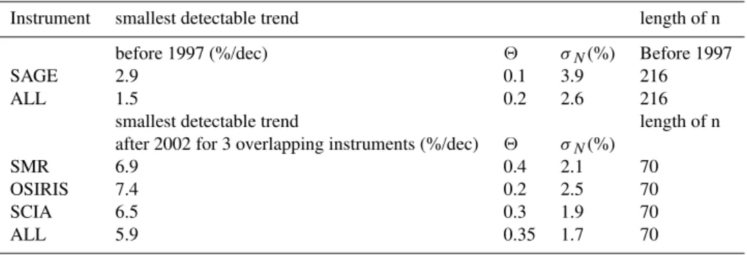
Table 4.Comparison of autocorrelation,2, standard deviation,σN,length of data set, and the smallest detectable trend for various individual instruments overlapping in time.
Instrument smallest detectable trend length of n
before 1997 (%/dec) 2 σN(%) Before 1997
SAGE 2.9 0.1 3.9 216
ALL 1.5 0.2 2.6 216
smallest detectable trend length of n after 2002 for 3 overlapping instruments (%/dec) 2 σN(%)
SMR 6.9 0.4 2.1 70
OSIRIS 7.4 0.2 2.5 70
SCIA 6.5 0.3 1.9 70
ALL 5.9 0.35 1.7 70
Table 4 presents results using data from the northern mid-latitudes between 35 and 45 km applying this method. The table gives information about the three statistical parame-ters for each time series and hence the smallest possible de-tectable trend for data up to and after 1997. Also presented are the all instrument average results highlighted in bold. Firstly, if one considers just the SAGE data for trend anal-ysis prior to 1997, one could obtain a minimum detectable linear trend of 2.9%/decade, using autocorrelation and stan-dard deviation of 0.1 and 3.9%, respectively. However, if we now include the contributions from the SBUV/2 and HALOE anomalies to the SAGE anomaly time series (hence, produc-ing the all instrument average) it can be seen that the standard deviation is reduced by about a third. The resulting smallest detectable trend in this case is 1.5%/decade, which is approx-imately a factor two smaller than if we were to utilize only the SAGE anomaly time series. Another example is shown in the lower part of Table 4. Here, a comparison is made with three instruments which overlap in time. In this case we use an overlap time for the present SCIAMACHY mission, with both Odin instruments, covering a total of 70 months (2002–2008 to 2008–2003). It should also be noted that both SMR and OSIRIS time series are longer than this, but data is here only considered where they overlap with the SCIA-MACHY data. Individually, instruments share similar noise levels of typically 2–3% and have autocorrelations varying from 0.2–0.4 The minimum detectable trend for each in-strument is 6.9%/decade for SMR, 7.4%/decade for OSIRIS, and 6.5%/decade for SCIAMACHY (at the two sigma level). However, by combining these individual time series we at-tain a less noisy time series and a smallest detectable trend of 5.9%/decade, which is smaller than if we were to just con-sider one single instrument time series.
As time series length is important, it is favored that a trend analysis shall use only the longest time series avail-able. However, by combining all data it is possible to use data sets that are much shorter as long as instrument drift (if any) is accounted for. The combination of overlapping data potentially gives a less noisy time series and the capability to
find a more reliable trend estimate, which is particularly use-ful for early as possible detection of ozone recovery based on an analysis with the more recently launched satellites (for example, Odin, Envisat, ACE, Aura). We have seen from the previous section that at present it is difficult to ascertain if ozone is truly recovering. We can however estimate how many more years of combined data utilizing SMR, OSIRIS, and SCIAMACHY are needed by knowing the autocorrela-tion and noise parameters of the all instrument average. If we consider the 30◦N–60◦N and 35–45 km trend value post
1997 (Table 1), we find that ozone is increasing (but not sig-nificantly), by 1.4±2.3% per decade. For this particular case the autocorrelation and noise values are 0.2 and 2.5%, re-spectively. Weatherhead et al. (1998) suggest that one can obtain the number of years needed in order to calculate a trend of choice based on Eq. (3),
n≈ σN
σw
r
1+θ
1−θ
!2/3
(3) Similarly to Eq. (2), Eq. (3) follows the non zero trend assumption, with 95% confidence corresponding to
|Wh/σw|>2. In this case the standard error, σw, is 1.15%/(half of the 2 sigma trend error), it implies that the ratio between the trend value and the standard error is only 1.2. As this ratio needs to be at least two it means that at the current rate of ozone increase we must have a maximumσw of no larger than 0.7%/decade. Assuming that the all instru-ment mean maintains the same noise and autocorrelation val-ues in the future,nwould equate to approximately 13 years calculated with aσwof this value. Hence, it would not be un-til at least 2010 where one could see a statistically significant 1.4%/decade increase in ozone.
5 Water vapour
1992 1994 1996 1998 2000 2002 2004 2006 2008 −10
0 10
1992 1994 1996 1998 2000 2002 2004 2006 2008
−10 0 10
Water vapour anomaly [%]
1992 1994 1996 1998 2000 2002 2004 2006 2008
−10 0 10
1992 1994 1996 1998 2000 2002 2004 2006 2008
−10 0 10
Year
D C B A
Fig. 7.Water vapour anomalies for four instruments for the 30◦S–30◦N and 25–35 km bin. Shown are the SAGE I+II (blue,A), HALOE
(red,B), SMR (magenta,C), MLS (black,D). Also shown under-laid is the all instrument average (green).
Figure 7 illustrates how each individual instrument con-tributes to the all instrument average (green line) for the 25– 35 km and 30◦S–30◦N bin once the respective anomalies are calculated. From October 1991 until January 1995 we only consider HALOE data as the SAGE II data are removed due to aerosol contamination. The main feature from 1991–1996 is a general increase in values until the middle of 1996 where values level off until 2002. HALOE and SAGE II values are by and large consistent with each other from 1995 un-til 2005 when each instrument ceased operation. After 2002 mean water vapour anomaly values drop, which is more pro-nounced in the HALOE data than in the SAGE II data. This result is in agreement with reports of a sudden decrease in water vapour values in the lower most stratosphere in 2001, which are coupled with a decreased tropical tropopause tem-perature (Randel et al., 2004, 2006). Perhaps most inter-estingly of all is the excellent agreement of SMR and MLS anomalies, which show a similar pronounced structure as the HALOE time series during their respective overlapping pe-riods (2001–2005, and 2004–2005 respectively), but are also less noisy due to their better spatial and temporal sampling of the emission sensors (SMR measures with global cover-age in approximately one day per week, while MLS mea-sures a global coverage daily). Not only does this confirm the drop in water vapour values seen previously using HALOE and other measuring techniques (such as the balloon sonde frost point hygrometer measurements at Boulder, Colorado), it more importantly shows how well the different measure-ments agree considering the different techniques used. Since
2005 we see that the combination of SMR and MLS show water vapour values to have increased and have reached con-centrations that are similar to values prior to the 2001/2002 drop.
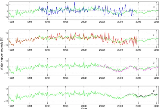
Figure 8 shows the all instrument average in all bins from October 1991 until April 2008. Also shown are the HALOE deseasonalised anomalies laid on top for reference. By con-sidering just the HALOE observations it is clear that there is an increase in water vapour from 1991 until 2001 in the 20– 25 km bin in the tropics (panel H), but is less evident else-where. The increase is seen in the lower stratosphere at mid-latitudes but is considerably less steep after 1996. Also illus-trated is a decrease in both 20–25 km mid-latitude bins (pan-els G and I), where anomaly values decrease after 2001, but are delayed by∼6 months, which is logical since there will be a time lag between the air passing out of the tropics and moving towards the poles. A larger time lag is also present in the extra-tropical 25–35 km altitude bins (panels D and F) as should be expected where a drop in values is seen typically
1995 2000 2005 −15
−10 −5 0 5 10 15
year 1995 2000 2005 −15
−10 −5 0 5 10 15
1995 2000 2005 −15
−10 −5 0 5 10 15
1995 2000 2005 −15
−10 −5 0 5 10 15
1995 2000 2005 −15
−10 −5 0 5 10 15
1995 2000 2005 −15
−10 −5 0 5 10 15
1995 2000 2005 −15
−10 −5 0 5 10 15
1995 2000 2005 −15
−10 −5 0 5 10 15
Residual water vapour [%]
1995 2000 2005 −15
−10 −5 0 5 10 15
A B C
D E
G H I
F
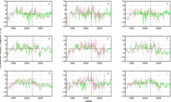
Fig. 8.All instrument average stratospheric water vapour anomaly time series (green) for nine altitude/latitude bands. Also shown overlaid
are the HALOE anomalies for comparison (pink).
As we have extended the water vapour time series until spring 2008, it is interesting to see that the post 2002 de-cline of water vapour anomalies has leveled off and in some cases values have increased. Anomalies reach minimum val-ues approximately between 2004 and 2006 in all bins except one (panel F). The tropical altitude bins (B, E, and H) ex-hibit large increases in water vapour values (between 3 and 7%), while panels B and H show similar values to those prior to 2002. Additionally, the 35–45 km mid-latitudes (panels A and C) have also seen smaller increases in water vapour values since 2005, although present values are generally still below pre 2002 values. It appears that the 25–35 km mid-latitude stratospheric bins (panels D and F) do not show a great deal of symmetry as it appears that the Southern Hemi-sphere recovers quicker and has generally larger values dur-ing the period of 2005–2008. Furthermore, bin F shows the smallest water vapour values at present, giving anomaly val-ues typically between−5 and−7%.
5.1 Discussion of water vapour results
As mentioned, Randel et al. (2006) showed water vapour to be strongly correlated to the Cold Point Temperature (CPT). The CPT is defined as the position in the temperature profile where the coldest temperature occurs (Zhou et al., 2001) and is found in the Tropical Tropopause Layer (TTL). Here, air is freeze dried as it is transported vertically from the tropo-sphere to the lower stratotropo-sphere, thus the cold point is a use-ful parameter for monitoring water vapour entering the lower stratosphere. Randel et al. (2006) showed that the reduction
of water vapour values after 2001 were complemented by a decline in CPT also believed to be associated with enhanced deep convection between 20◦S and 20◦N (Rosenlof et al., 2008). A further explanation is that TTL temperatures are thought to be driven by the Brewer Dobson circulation (Ran-del et al., 2004; Nedoluha, 2002). Dhomse et al. (2008) illustrates this by using the eddy heat flux (a parameter for planetary wave activity) and find an anti-correlation when compared to SAGE II, HALOE, and POAM water vapour concentrations seen in the lower tropical stratosphere. Fur-thermore, the authors report that from 2000 to 2005 the Brewer Dobson circulation was stronger than normal due to enhanced planetary wave activity. This is suggested to be a result of enhanced mixing in the extra-tropics, leading to additional air being drawn from the lower stratospheric trop-ics, causing cooling in the tropical tropopause region due to adiabatic expansion and thus reducing water vapour values.
2001 2002 2003 2004 2005 2006 2007 2008 −2
−1 0 1 2
Year
Temperature anomaly [%]
2001 2002 2003 2004 2005 2006 2007 2008
−10 −5 0 5 10
Year
Water vapour anomaly [%]
Fig. 9.Top: ECMWF temperature anomalies measured at 100 hPa and between 20◦S and 20◦N (red). Overlaid is the five month running
mean of the same data (green). Bottom, the water vapour all instrument average for 30◦S–30◦N and 20–25 km. Overlaid is the five month running mean of the same data (green).
(green line) illustrates a clear change from a negative to a positive trend of temperature after 2004. This agrees with the increase of water vapour anomalies seen in the lower panel after 2004 (also visible in the 25–35 km tropical bin shown in panel E, Fig. 8). This could imply that the enhanced plane-tary wave activity slows down after 2005 allowing a gradual increase of CPT and a reduction of water vapour entering firstly in the tropics and then eventually in mid-latitudes. It could also imply that the period of deep convection seen in the tropics is possibly over. However, the increase in wet-ness is not monotonic as exemplified by Fig. 9 (lower panel) where more negative anomalies are seen in 2005 and 2007. Finally the increase in water vapour anomalies after 2004 in the extra-tropical upper stratosphere (∼3%) seen in panels A, and C in Fig. 8 could also be explained by the photodissoci-ation of methane to water vapour although this is thought to only contribute∼0.5%/year (Nedoluha et al., 2003). Further-more the global increase of methane has varied from about 14 ppb/year in 1985 to almost zero in 2000 in the stratosphere (but with a high degree of natural variability). Since 2000 the growth rate of methane is estimated to be 0±4 ppb/year (WMO, 2006). This would also suggest that methane’s con-tribution to the increase in water vapour values during the 2004–2008 period is small, given that the mean age of air at those altitudes and latitudes is typically 6–8 years (Stiller et al., 2007).
6 Summary
We have extended the stratospheric ozone and water vapour time series until April 2008 by adding recent satellite data. We have examined the long term evolution of both species in nine separate global bins covering 60◦S and 60◦N and
be-tween 20 and 45 km. We applied a linear regression model to each instrument monthly mean time series in order to remove contributions of seasonal, QBO and solar cycles. We com-bined all individual instrument’s remaining anomalies and constructed an all instrument mean.
values would be reached in approximately 70 years, hence the latter part of the mid 21st century, which is later than the near linear model estimates of 2040–2050 presented by the WMO (2006). However, as the post 1997 all instrument average anomalies in these two bins are not statistically sig-nificant to a 95% level of confidence it means more time is needed in order to ascertain that an authentic ozone recovery has occurred.
We also show that the assumption that the year where a change in ozone trend is believed to occur was not neces-sarily always the same for all latitudes and altitudes. As we assume the linear regression model suggested by Rein-sel et al. (2002), such that the turn around is an immediate change in trend, it produces turn around times earlier than 1997, which is the suggested turn around time using either the EESC or CUSUM method. We find turn around times to range between 1994 and 1996, although we see no obvious relationship between the upper and lower stratosphere. By using this method on the all instrument average anomalies we can not conclude that a recovery is more likely to occur earlier in the upper stratosphere, as suggested by Jucks et al. (1996).
An all instrument mean is also calculated for water vapour using four instruments, SAGE II, HALOE, SMR, and MLS. As we find little point in making a trend prognosis due to highly variable anomaly time series in each bin, we have de-cided instead to focus more on the period after 2001 where a drier stratosphere has been seen (Nedoluha et al., 2003; Ran-del et al., 2004, 2006). We see similar characteristics to the above studies in the lowest tropical altitude bin (20–25 km), although the extra-tropics in this altitude range see the de-cline∼6–18 months later, which is the expected time lag as air is transported from the tropics to the mid-latitudes (Stiller et al., 2007). In the middle stratospheric bins (25–35 km) the drop is found∼12–18 months after 2001, and a similar delay is seen in the upper stratospheric tropical and extra-tropical bins (35–45 km). Since 2004–2005 water vapour concentra-tions have generally been steady, while some bins have even shown signs of increasing values. The largest increase in wa-ter vapour values is calculated to be in the lowest tropical bin (20–25 km), where present values are typically similar to those prior to 2002. We also show the ECMWF 100 hPa temperature anomaly from 2001 to 2008, where we find a change in the trend sign occurs around 2004–2005 indicat-ing an increasindicat-ing temperature until present, although there is high level of variability. The temperature from this pressure level is a good indicator of the CPT and hence correlated to the amount of water entering the stratosphere (Zhou et al., 2001).
Finally, even though the all instrument average is a com-bination of several instruments and different measurement techniques it provides a strong basis for trend research. A robust trend analysis can only be made if the anomaly time series is long enough and is characterized by low noise, and low variability. Hence, using an all instrument mean can
provide a more precise estimate of trend as it can combine differing time domains as well as reduce the stochastic noise from individual data sets. The main requirement for con-structing such a time series is that there are at least a couple of years of overlap between data sets. Of course long indi-vidual time series such as those offered by SAGE II, SBUV/2 and HALOE are preferable but even the shorter time series that are known to have little long term drift can also be in-cluded for the purposes of long term trend analyses similar to that shown here.
Acknowledgements. Odin is a Swedish-led satellite project funded
jointly by the Swedish National Space Board (SNSB), the Canadian Space Agency (CSA), the National Technology Agency of Finland (Tekes) and the Centre National d’Etudes Spatiales (CNES) in France. We would like to thank Larry Thomason and the Langley air research centre (NASA) for help regarding the SAGE data. We are also grateful for the HALOE, MLS (Alyn Lambert and L. Froidevaux) and SBUV/2 data also provided by NASA. Our thanks go to those at the European Space Agency (ESA) for providing SCIAMACHY, and funding the Odin products. SCIAMACHY is jointly funded by Germany, the Netherlands, and Belgium. SCIAMACHY data analysis at the University of Bremen is funded by DLR (50EE0727) and ESA (SCIAMACHY Quality Working Group). The IUP Bremen group and ourselves would like to thank the European Centre for Medium-Range Weather Forecasts (ECMWF) for providing pressure and temperature information. Some data shown here are were calculated on German HLRN (High-Performance Computer Center North) and NIC/JUMP (Jlich Multiprocessor System). Services and support are gratefully acknowledged.
Edited by: P. Hartogh
References
Baldwin, M. P., Gray, L. J., Dunkerton, T. J., Hamilton, K., Haynes, P. H., Randel, W. J., Holton, J. R., Alexander, M. J., Hirota, I., Horinouchi, T., Jones, D. B. A., Kinnersley, J. S., Marquardt, C., Sato, K., and Takahashi, M.: The Quasi-Biennial Oscillation, Rev. Geophys., 39, 179–229, 2001.
Bhartia, P. K.: Total ozone from backscattered ultraviolet measure-ments, in Observing Systems for Atmospheric Composition, 48– 63, Springer Science, New York, 2007.
Bhartia, P. K., Wellemeyer, C., Taylor, S. L., Nath, N., and Gopalan, A.: Solar Backscatter UltraViolet (SBUV) Version 8 profile algo-rithm, In proceedings of the XX Quadrennial Ozone Symposium, edited by: Zerefos, Z., 295–296, Univ. of Athens, Greece, 2004. Bhartia, P. K., McPeters, R. D., Mateer, C. L., Flynn, L. E., and Wellemeyer, C.: Algorithm for the estimation of vertical ozone profiles from the backscatterd ultraviolet technique, J. Geophys. Res., 101, 18793–18806, 1996.
Bovensmann, H., Burrows, J. P., Buchwitz, M., Frerick, J., No¨el, S., Rozanov, V. V., Chance, K. V., and Goede, A. H. P.: SCIA-MACHY – Mission objectives and measurement modes, J. At-mos. Sci., 56(2), 127–150, 1999.