J. Microw. Optoelectron. Electromagn. Appl. vol.15 número4

Abstract— _{The purpose of this article is based on analyzing the use} of RTQ3D (“quasi-3D” ray tracing technique) to produce the value of the initial electromagnetic fields or fitness for a hundred and sixty receivers according to the possible positions of two antennas to be distributed in a closed environment. The problem variables consist of the values of the magnetic fields for one hundred and sixty receptors depending on the positions of the antennas to the base stations, which serve as input data for the algorithm to the RMLP (Artificial Neural Network, multilayer perceptron with Real backpropagation learning algorithm)

.

Index Terms— _{Artificial Neural Networks, Multilayer Perceptron,} electromagnetic fields, Particle Swarm Optimization, metamodeling.

I. INTRODUCTION

Optimization problems are characterized by situations in which one needs to maximize or minimize a

numerical function of several variables, in a context where there may be restrictions.

The sophistication of computer resources developed in recent years has motivated a breakthrough in

optimization techniques. In fact, optimization problems have become increasingly complex,

increasing the associated computational cost. Classical optimization techniques are reliable and have

applications in many different fields of engineering and other sciences. However, deterministic

methods can present some numerical difficulties and problems related to robustness: the lack of

continuity of the functions to be optimized or its constraints, nonconvex functions, multimodality, the

existence of noise functions, the need to work with discrete values for variables, the existence of local

minimum or maximum, etc. Thus, studies of heuristic methods with search-controlled randomized

Use of an Artificial Neural Network

-

based

Metamodel to Reduce the Computational Cost

in a Ray

-

tracing Prediction Model

Sheila S. Travessa, Walter P. Carpes Jr.,

Federal University of Santa Catarina, Electric Engineering Department Grupo de Concepção e Análise de Dispositivos Eletromagnéticos (GRUCAD)

Florianópolis, Brazil

probabilistic criteria reappear as a strong trend in recent years, mainly due to their robustness and to

the advancement of computational resources. One of the main motivations for using stochastic

optimization methods, such as PSO, is their ability to converge to the global optimum point. Indeed,

most of the electromagnetics problems are multimodal, and using a deterministic method could lead to

a local optimum. However, a limiting factor of stochastic methods is the need for a large number of

objective function evaluations [1].

In the methods of natural optimization, the objective function is evaluated several times, since we

deal with a great number of points (population) at a given iteration. This increases the computational

cost associated with these methods. However, this high computational cost is the price to pay for

preventing solutions from becoming trapped in local minima.

In general, the methods of natural optimization require more computational effort when compared

to classical methods, but have some advantages such as ease of implementation, robustness and do not

require continuity of the objective function associated with the problem [2].

An important application of metamodels is in the optimization of electromagnetic problems. In fact,

given that the modeling of such problems generally has a high computational cost, the optimization of

electromagnetic devices often requires certain procedures for the replacement of objective functions,

in order to evaluate them in an efficient way. The replacement function allows obtaining results with

good precision, but with a much lower computational cost [3].

Several models can be used to obtain approximations of objective functions with good accuracy.

The most popular are the polynomial model, Kriging model, feedforward neural networks, including

multilayer perceptrons, radial basis function networks and support vector machines. According to [4],

the development of strategies for assisted metamodels are proposed as a new approach to basic

simulation optimization in the field of electromagnetic project. In this application field, the estimation

of objective functions are likely to have a significant computational cost, and techniques such as

metamodeling are applied to accelerate the evolutionary optimization strategies. Some experiments

done with the main metamodels mentioned in this study showed that better results were obtained with

the Kriging model and artificial neural network.

The Kriging model [3] and the feed-forward neural network are robust and offer savings in

computational time. Studies have shown that these two metamodels have similar performance [5].

Therefore, we chose to use the Artificial Neural Networks (ANN), which have been widely used in

several applications due to ease of implementation and effectiveness.

It is important to stress that the evolutionary algorithms associated with metamodels are becoming

extensively used by a growing number of researchers in design optimization [6]. Here, we show the

validity of the PSO (Particle Swarm Optimization) algorithm in conjunction with an ANN-based

II. PSO, RTQ3D AND THE ANN-BASED METAMODEL

A. PSO – Particle Swarm Optimization

Introduced by Kennedy and Eberhart in 1995, the particle swarm optimization has emerged from

experiments with algorithms modeled from the observation of social behavior of certain types of

birds. The particles considered by the algorithm behave like birds looking for food or a place to make

their nests, each one using both its own knowledge and the knowledge of the flock (or swarm)

concerned to the best location for that. PSO is composed of particles represented by vectors defining

the current speed of each particle and its location. The location of each particle is updated according

to its current speed, its own knowledge and the knowledge acquired by the whole flock. The PSO

algorithm encompasses simple concepts and can be implemented in a few lines of code, requiring

only simple mathematical operators.

The algorithm starts by generating a population of N particles that form the swarm and establish

(randomly) their respective positions in the search space. It also sets the initial speed for each particle.

Subsequently, at each iteration k, the algorithm updates the position xi(k) and the velocity vi(k) of each

particle i. After the first evaluation of the fitness associated to a given particle, the algorithm keeps

track of the coordinates pi in the search space associated with its best solution. The overall best value

(considering the whole population) and its location ps(k) are also stored during the procedure. With a

simple scheme, these stored data are iteratively updated using random parameters and constants,

changing the particles velocities in order to intelligently explore the search domain at each iteration

[7].

The velocity vector of each particle is updated according to (1):





 



 





   



vi 1  i  1 1 i i  2 2 s  i (1)

Where w is the inertia weight; c1 and c2 are, respectively, the cognition and social coefficient; and r1

and r2 are random numbers uniformly distributed in [0,1]. Inertia weight w usually is chosen between

0.4 and 1.4: lower values speed up convergence while higher values encourage exploring the search

space. The value used for w in this study was 0.9, which allows obtaining very good results for the

analyzed problem. Cognition coefficient c1 limits the size of the step that the particle takes toward its

individual best while social coefficient c2 limits the size of the step that the particle takes toward the global best. Usually both assume values close to 2. It would be possible to use different values of c1,

c2 and w, including the idea of using variable parameters in time (e.g., decreasing w with the

advancement of iterations). This could have been done to improve the convergence. However, we use

typical fixed values for these parameters, according to the literature, which also yields satisfactory

results.

The position of each particle is updated according to (2):





  



xi i i (2)

The iterations proceed until some stopping criterion is reached (e.g., maximum number of iterations

B. An RTQ3D-indoor

For the purpose presented in this paper, the RTQ3D-indoor algorithm is used for field computation

and coverage evaluation, since the applications are in indoor environments. The RTQ3D-indoor [8]

model uses 2D ray-tracing algorithm based on the Theory of Images to build a “tree of images” and to

find the different reflected rays for a given scenario. The input scenario database is described in the

horizontal plane, but adding the ceiling height from the floor and the transmitting (base stations) and

receiving (user terminals) antennas heights [9].

According to the example of Fig. 1, the ray-tracing algorithm applied on quasi three-dimensional

indoor environments (RTQ3D-indoor) converts a given path initially obtained from the RT 2D

algorithm in five rays: i) the direct path (from the viewpoint of a vertical plane); ii) the ground

reflected path; iii) the ceiling reflected path; iv) the path reflected on the ground and on the ceiling

and; v) the path reflected firstly on the ceiling and then on the ground [9].

Fig. 1. Passage of a 2D path to five quasi-3D paths using the RTQ3D-indoor algorithm [8]: a) horizontal plane; b) vertical plane [9].

C. Metamodel: ANN (Artificial Neural Network) with backpropagation algorithm

According to [10], a neural network is a massively parallel distributed processor consisting of

simple processing units, which have the natural tendency for storing experiential knowledge and

making it available for use. It resembles the brain in two respects:

- knowledge is acquired by the network from its environment through a learning process;

- connection strengths between neurons, known as synaptic weights, are used to store the

acquired knowledge.

to modify the synaptic weights of the network in a systematic manner to achieve a desired design

goal. We consider the multilayer perceptron (MLP), which consists in a network of simple neurons

called perceptrons. The MLP is a hierarchical structure of several perceptrons with some advantages

compared to single-layer networks and it is capable of learning a rich variety of nonlinear decision

surfaces [10-11].

The so-called neuron's net input can be represented by the weighted sum of the inputs from other

neurons and external inputs, according to (3).





 

 

  p

j

m

l

i k ki j

ji

i t w y t w I t

net

1 1

) ( )

1 ( )

(  (3)

Where yj(t – 1) is the output of the j-th neuron in the previous processing cycle (t-1); Ik is the k-th

external input; θi is the bias of the i-th neuron and w refers to the corresponding weight, shown in

Fig.2[10].

Fig.2. Illustrative “Graph” of The proposed network [10].

In order to model an electromagnetic problem, data from the electromagnetic simulation are used to

train the ANN, i.e., to compute the weights of (3). Here, we chose to use the backpropagation (BP)

algorithm for this training (supervised learning). Backpropagation is an abbreviation for "backward

propagation of errors". In the BP algorithm, the network begins with a random set of weights. Input

data is normalized to a range of ±1 and input vectors are presented to the network. Thus, the

corresponding output is calculated using the initial weight matrix. Next, the ANN output is compared

to the output of the electromagnetic simulation (using the same input data). The squared difference

between the two output vectors determines the system error. The accumulated error for all of the

input-output pairs is defined as the Euclidean distance in the weight space which the network attempts

to minimize. Minimization is accomplished via a gradient descent approach, in which the weights are

adjusted in the direction of decreasing error. When the error has been decreased below a pre-defined

with units that use nonlinear activation functions. Since the BP algorithm requires an activation

function to be differentiable, we used a sigmoid (logistic function) [10]. Another important aspect in

defining the topology of neural network is the number of neurons in the hidden layer, due to its

influence on both the speed and the effectiveness of the learning network, which was defined by the

geometric mean between the input and output neurons [11].

III. VALIDATION

In order to verify the effectiveness of proposed method, it was initially used in the optimization of a

test function with analytical solution. Specifically, the goal is to find the global maximum of the

Peaks function, given by (4) and shown in Fig. 3. It is important to mention that the Rastrigin and

Sinc functions were also tested during the validation process of this study, with satisfactory and

similar results for all of them. The results obtained through the functions Peaks, Rastring and Sinc

showed the efficiency and effectiveness necessary to validate the proposed PSO optimizer assisted by an ANN.

   





3 1 2 2 5 10 3 10 2 2 1 2 2 1

3 x e x y x x y e x y e x y

x,y

F               

          (4)

Fig.3. The analytical function considered.

The goal of this implementation is to test the effectiveness of the PSO optimizer using an ANN

(network MLP with backpropagation algorithm) as a metamodel.

The optimization was done both directly using the function given by (4) and using an ANN-based

metamodel to represent it. Specifically, the PSO was used to obtain the global maximum location of

Peaks function. The algorithm was initialized with a random set of particles and the process took

place until the maximum point was located, at the center of the red contours.

Fig. 4(a) shows the contour plot of the results obtained using directly (4) while fig. 4(b) shows the

(a)

(b)

Fig.4. (a). Contour plot of the actual function; (b) Contour plot of the simulated function, with the located peak.

The ANN was trained until a root mean square error of 0.0004 was obtained, requiring 27,253

epochs to get this error value. An epoch is a step in the training process of an ANN, i.e., each time the

network is presented with a new input pattern. The root mean square error solution of PSO assisted by

the ANN was equal to 0.00569. From the results, we can conclude that the use of the proposed

metamodel to replace the original fitness function allows obtaining good results.

IV. ELECTROMAGNETIC PROBLEM

The use of an electromagnetic prediction model represents an important design procedure in

wireless systems. Here, we use a quasi-3D ray-tracing propagation model associated with a PSO

optimizer to find optimal antenna placement in an indoor scenario [9-11].

Initially, a population is generated where each particle corresponds to the coordinates (x, y) of the

-3 -2 -1 0 1 2 3

-3 -2 -1 0 1 2 3

X

Y

X

Y

-3 -2 -1 0 1 2 3

transmitting antennas placements in a 40 m × 28 m scenario. It was defined a mesh of 160 receptors

uniformly distributed within the environment. The antennas of all receivers were considered to be 1.5

m high from the ground. The method was applied to minimize the number of points where the field is

below a minimum reception threshold (-110 dBm). This is equivalent to maximize the coverage area.

The variable of the problem was assumed to be a vector containing the coordinates (x, y) of the

transmitting antennas, allowing different locations of them on the horizontal plane of the scenario.

The height of these transmitting antennas was assumed to be fixed (3 m), simulating vertically

polarized quarter-wave monopole antennas fixed to the ceiling. Two antennas were considered in the

problem. Therefore, the variable of the problem is a vector containing four elements, which represent

coordinates of transmitting antenna positions on the horizontal plane. The frequency used was 2.4

GHz, and the total equivalent isotropically radiated power (EIRP) was 400 mW.

Firstly, the field values generated by ray-tracing are used as a guide in the learning process

performed by the network, optimizing weight values, which are saved in a file. After training, the

ANN calculates the field values at all reception points, which are used by the PSO optimizer, allowing

a great reduction in computation time.

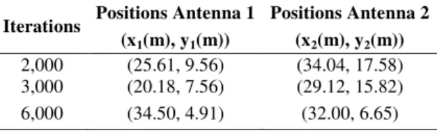
The PSO assisted by ANN was initialized with a set of 100 random particles. The PSO assisted by

ANN optimizing was performed for three different numbers of iterations: 2,000, 3,000 and 6,000.

Table I shows the best antenna locations found by the PSO for these three cases. We observe that the

results are very sensitive to the number of iterations, which indicates that the ANN needs to be further

improved. Fig. 5 shows the mapping of received powers considering the best pair of positions of the

antennas found for 3,000 iterations. We see that the distribution of field is reasonable. Best results,

with more uniform fields, can be obtained using more transmitting antennas in the scenario.

TABLE I. RESULTS OF OPTIMIZATION ANN-ASSISTED PSO

Iterations Positions Antenna 1 (x1(m), y1(m))

Positions Antenna 2 (x2(m), y2(m))

Fig.5. Received power mapping in the indoor environment (3,000 iteractions).

V. CONCLUSIONS

In this paper, we proposed a PSO optimizer assisted by an ANN, the optimizer was implemented using the MATLAB program version 7.10.0.499. The optimization process was carried out through a MacBook Pro Retina Computer with 2,6 GHz intel Core i5 processor and 8GB of RAM memory 1600MHz DDR3, with 256GB of flash storage. In the optimization of an electromagnetic problem, the computational cost can be very large, since it is necessary to carry out a numerical simulation for each evaluation of the fitness function. In this case, the use of an ANN as a metamodel permits to obtain satisfactory results with a reduction of the computational cost. The study developed in this work is based on [9], where the association of RTQ3D-indoor with PSO optimizers was applied in a

typical telecommunication problem: a wireless local area network (WLAN) system in an indoor

scenario that must be covered with two 802.11b/g/n (2.4 GHz) access points (AP). However, the study

developed in [9] disregards the computational cost, which is quite high when a metamodel is not used.

As an example, the average time required for optimization using the ANN metamodel with 3,000

epochs is around 36 min. Without using the metamodel, the PSO takes about 72 hours to produce

slightly better results.

In order to assess the effectiveness of the proposed method, it was applied in a test function with a global maximum. Also, it was applied in an electromagnetic problem (namely, the best antenna positioning in wireless systems). The response of the ANN-assisted PSO for a real electromagnetic problem can be considered satisfactory. All observations suggest that an improvement in the ANN and additional training will lead to the best results. However, this would increase the computational

REFERENCES

[1] H.P. Schwefel, E. L. Taylor, “Evolution and Optimum Seeking,” John Wiley & Sons. Inc, United States of America, pp. 87-88, 1994. [2] G. Venter, and J. Sobieszczanski-sobieski, “Particle Swarm Optimization,” Proceedings of the 43rd AIAA/ASME/ASCE/AHS/ASC

Strutures, Structural Dynamics, and Materials Conference, Denver, CO, Vol. AIAA-2002-1235, April 22-25 2002.

[3] L. Lebensztjan, C. A. R. Marretto, M. C. Costa, J. L. Coulomb, “Kriging: a useful tool for electromagnetic device optimization,” vol.40, No_{.2. IEEE Transactions on Magnetics, March 2004, p. 1196-99.}

[4] M. T. M. Emmerich, C. M. Varcol, “Metamodel–Assisted Evolution Strategies in Electromagnetic Compatibility Design,” EUROGEN. 1-12, 2005.

[5] L. Willmes, T. Bäck, Y. Jin, “Sendhoff, B. Comparing neural network and kriging for fitness approximation in evolutionary optimization,” IEEE, 2003 pp. 670.

[6] Y. Rahmat-Samii, N. Jin, “Particle Swarm Optimization (PSO) in Engineering Electromagnetics: A Nature-Inspired Evolutionary Algorithm,” IEEE, 2007. Inc, United States of America, 1994 pp. 87-88.

[7] R. C. Eberhart and Y. Shi, “Particle Swarm Optimization: Developments, Applications and Resources,”Congress on Evolutionary Computation, 2001, vol. 1, pp. 81-86, 2001.

[8] S. Grubisic, W. P. Carpes Jr, J. P. A. Bastos, “An Efficient indoor ray- tracing propagation model with a quasi-3D approach,” IEEE CEFC 2012, November 2012, Oita/Japan.

[9] S. Grubisic, W. P. Carpes Jr, J. P. A. Bastos, G. Santos, “Association of a PSO optimizer with a quasi-3D ray-tracing propagation model for mono and multi-criterion antenna positioning in indoor environments,” IEEE Transactions on Magnetics, Vol. 49, No. 5, May 2013.

[10] S. Haykin, “Neural Networks: A Comprehensive Foundation,” Prentice Hall, 1999.