Abstract
In this paper, the Equivalent Linearization Method (ELM) with a weighted averaging, which is proposed by Anh (Anh, 2015), is applied to analyze some vibrating systems with nonlinearities. The strongly nonlinear Duffing oscillator with third, fifth, and seventh powers of the amplitude, the other strongly nonlinear oscillators and the cubic Duffing with discontinuity are considered. The re-sults obtained via this method are compared with the ones achieved by the Min-Max Approach (MMA), the Modified Lindstedt – Poin-care Method (MLPM), the Parameter – Expansion Method (PEM), the Homotopy Perturbation Method (HPM) and 4th order Runge-Kutta method. The obtained results demonstrate that this method is very convenient for solving nonlinear equations and also can be successfully exerted to a lot of practical engineering and physical problems.
Keywords
nonlinear oscillator, Equivalent Linearization Method, weighted averaging.
The Equivalent Linearization Method with a Weighted
Averaging for Analyzing of Nonlinear Vibrating Systems
1 INTRODUCTION
Nonlinear oscillations systems are such phenomena that mostly occur nonlinearly. These systems are important in engineering because many practical engineering components consist of vibrating sys-tems that can be modeled using oscillator syssys-tems such as elastic beams supported by two springs or mass-on-moving belt or nonlinear pendulum and vibration of a milling machine. Hence solving of governing equations and due to a limitation of existing exact solutions have been one of the most time-consuming and difficult affairs among researchers of vibrations.
The amplitude–frequency relationship is of significant importance for the accurate prediction of nonlinear oscillator systems in many areas of physics and engineering, especially in nonlinear struc-tural dynamics. Therefore, the analyzing of nonlinear systems has been widely considered. In recent years, many powerful methods are used to find approximate solution as well as the
amplitude-N. D. Anh a N. Q. Hai b D. V. Hieu c
a Institute of Mechanics, Ha Noi, Viet Nam. Email: [email protected] b Ha Noi Architechtural University, Ha Noi, Viet Nam. Email:
c Thai Nguyen University of Technology, Thai Nguyen, Viet Nam. Email:
http://dx.doi.org/10.1590/1679-78253488
frequency relationship to the nonlinear differential equations. Some of these methods are Ho-motopy Perturbation Method (HPM) (He, 1999; He, 2004a; He, 2004b; He, 2004c; Turgut et al., 2007; Bayat et al., 2012), Max-Min Approach (MMA) (He, 2008; Ganji et al., 2010; Chen et al., 2011; Dumaz et al., 2011; Yazdi et al., 2012; Bayat et al., 2012), Variational Iteration Method (VIM) (Bayat et al., 2012), Energy Balance Method (EBM) (Ganji et al., 2009; Khah et al., 2010; Younesian et al., 2010; Bayat et al., 2012), Amplitude-Frequency Formulation (AFF) (Chen et al., 2011; Jouyburi et al., 2014; Bayat et al., 2012), Parameter Expansion Method (PEM) (Kayaa et al., 2009; Dumaz et al., 2011; Darvishia et al., 2008; Zhao, 2009; Bayat et al., 2012 ), Homotopy Analy-sis Method (HAM) (He, 2004c; Bayat et al., 2012, Shahram Shahlaei-Far et al., 2016), Modified Homotopy Perturbation Method (MHPM) (Jouybari et al., 2014), Equivalent linearization Method (ELM) (Krylov et al., 1943; Caughey, 1959; Iyengar, 1988; Anh et al., 1995; Anh et al., 1997; Eli-shakoff et al., 2009; Anh, 2015) and combining Newton’s Method with the Harmonic Balance Meth-od (Lim et al., 2006).
The Equivalent Linearization Method of Kryloff and Bogoliubov (Krylov et al., 1943) was gen-eralized to the case of nonlinear dynamic systems with random excitation by Caughey (Caughey, 1959). And then, this method has been developed by many authors (Iyengar, 1988; Anh et al., 1995; Anh et al., 1997; Elishakoff et al., 2009). It has been shown that the Gaussian equivalent lineariza-tion is presently the simplest tool widely used for analyzing nonlinear stochastic problems. Never-theless, the accuracy of the Equivalent Linearization Method with conventional averaging normally reduces for middle or strong nonlinear systems. A reason is that some terms will vanish in the
aver-aging process, for example the averaver-aging value of the functions sin(t) and cos(t) over one period is
equal to zero. Anh N. D. (Anh, 2015) proposed a new way for determining averaging values, instead of using conventional averaging process author introduced weighted coefficient functions.
In this paper, the equivalent linearization method with weighted averaging is applied to nonlin-ear oscillators. To illustrate the applicability and accuracy of the method, four examples are pre-sented: nonlinear Duffing oscillator with third, fifth, and seventh powers of the amplitude, the
strongly nonlinear oscillators and the cubic Duffing with discontinuity. The amplitude–frequency
relationship can be readily obtained by this method. The results compared with the ones given by the numerical method and other well-known techniques show the accuracy of this method.
2 THE EQUIVALENT LINEARIZATION METHOD WITH A WEIGHTED AVERAGING
2.1 The Equivalent Linearization Method
In order to present the general idea of the equivalent linearization method, we consider a nonlinear oscillator governed by the following equation:
2 0
2 ( , ) 0
X h X X g X X (1)
where g X X( , ) is a nonlinear function only depending on two variables of velocity X t( ) and
dis-placement X t( ), h and 0 are constants. The corresponding equivalent linear oscillator is described
by the equation as follows:
2 0
(2 ) ( ) 0
The equation error between the two oscillators is taken as
( , ) ( , )
e X X g X X X X (3)
The coefficients of linearization in the linearized Eq. (3) are found from a certain optimal crite-rion. There are some criteria for determining these coefficients. The most common criterion is the mean square error criterion which requires the mean square of equation error to be minimum:
22
,
( , )
( , )
e X X
g X X
X
X
Min
(4)Thus, from
2
2
( , ) 0 ( , ) 0 e X X e X X
it follows that
2
2
2 2
g X X g X X X
X X X X
(5a)
2
2
2 2
g X X g X X X
X X X X
(5b)
In the formulas in Eqs. (4) and (5), the symbol denotes the time-averaging operator in
clas-sical meaning:
0
1
( )
lim
T( )
T
f t
f t dt
T
(6)For a ω-frequency function f(ωt), the averaging process is taken during one period T, i.e. 2 0 0
1
1
( )
( )
( ) ,
2
Tf
t
f
t dt
f
d
t
T
(7)2.2 The Weighted Averaging
It is well-known that for a given data set the most common statistic is the arithmetic mean. The concept for the average of a data set can be extended to functions. The conventional average value of an integrable deterministic function x(t) on a domain D: (0,d) is a constant value defined by:
0 1 ( ) d ( )
x t x t dt
d
(8)In many cases when the function x(ωt) is periodic with period 2π/ω, the value d is taken as
2π/ω and it leads to the averaged value of x(t) over one period:
2 / 2
0 0
1
( ) ( ) ( )
2 2
x
t
x
t dt x
d
(9)where
t
is the new variable or “new time”. Averaged values play surely major roles in the pastand at present, however, the definition (8) has some deficiencies, for example, if (8) or (9) are equal zero, the information about x(t) will be lost. For all harmonic functions cos(nωt) and sin(nωt), this observation is true. The dual approach to averaged values may be a possible way to suggest an
alternative choice for the conventional average value, namely the constant coefficient 1/d in Eq. (8)
can be extended to a weighted coefficient as a function h(t). Thus one gets so-called a weighted
average value:
0
( ( )) d ( ) ( )
W x t
h t x t dt (10)where the condition of normalization is satisfied:
0 ( ) 1
d
h t dt
(11)There are three basic weighted coefficients:
+ Basic optimistic weighted coefficients: They are increasing functions of t and denoted as O(t).
Examples are t and t
e
, , > 0.
+ Basic pessimistic weighted coefficients: They are decreasing functions of t and denoted as
P(t). Examples are t and t
e
, < 0, > 0; or > 0, < 0.
+ Neutral weighted coefficients: They are denoted as N(t) and are constants.
An arbitrary weighted coefficient h(t) can be obtained as summation and/or product of basic
weighted coefficients. Example is:
1
( ) n i i( ) i i( ) i i( ) ( )i ( )
i
h t A O t B P t C O t P t N t
(12)where A B Ci, ,i i are constant.
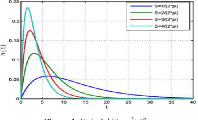
In this paper, we will consider only ω-periodic functions x(ωt). A special form of weighting coef-ficient is introduced as:
2 2
( ) s t, 0
where s is constant.
Figure 1: Plot of ( ) 2 st
h t s te .
It is seen that the weighting coefficient (13), obtained as a product of the optimistic weighting coefficient t and the pessimistic weighting coefficient e–sωt, has one maximal value at tmax 1 / ( )s ,
and then decreases to zero as
t
(see Fig. 1). If one requires that the time tmax is equal toT/n=2π/(nω) where n is a natural number or zero, we get s=n/(2π). So the meaning of s can be
specified as follows: for n = 1, s=1/(2π) the weighting coefficient (13) has maximal value after one
period, and for n=4, s=4/(2π) the weighting coefficient (13) has maximal value after quarter
peri-od, and for n=0, s=0 the weighting coefficient (13) has maximal value at infinity. This case
corre-sponds to the conventional averaged value.
Based on the weighting coefficient (13), a new weighted average value is proposed:
2 2 2
0 0
( )
s t( )
s( )
x t
s
te
x t dt
s e x
d
(14)which is a linear operator. From Laplace transformation, we get, for example:
2 2
2 2 2 2
2 2 2
0 0
cos( )
cos( )
cos( )
(
)
s t s
s
n
n t
s
te
n t dt
s e
n d
s
s
n
(15)2 2 2 2
2 2 2
0 0
2
sin( )
sin( )
sin( )
(
)
s t s
sn
n t
s
te
n t dt
s e
n d
s
s
n
(16)As ω-periodic functions x(ωt) can be expanded into Fourier series, hence we can easy calculate
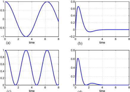
Figure 2: Graphs of the function: (a) - cos(τ), (b) - h(τ)cos(τ), (c) – cos2(τ), and (d) - h(τ)cos2(τ).
The proposed averaging operation can preserve the linear properties of the classical one. Fur-thermore, it can conserve some terms which vanish in the classical averaging process. The effect of the weighted function to the averaging process can be recognized, for instance, when we observe the graphs of functions cos(τ), h(τ)cos(τ), cos2(τ), and h(τ)cos2(τ) in Fig. 2. The function h(τ) adjusts the value of the functions cos(τ) and cos2(τ), maintains partly the periodicities of the functions
cos(τ) and cos2(τ), also condenses these function values in the first period, gives a weight in the first half of the first period, reduces the difference maximum and minimum values as well as regulates the functions during the period. These adjustments may make a positive effect on the averaging process. Therefore, the linearized equation replacement for the original one may be better in some senses.
In this paper, for the sake of computation convenience, the parameter s is chosen equal to 2.
3 SOME EXAMPLES AND DISCUSSIONS
3.1 Example 1
We consider the strongly nonlinear Duffing oscillator with third-, fifth-, and seventh-order nonlinear terms in the following form:
3 5 7 0
uuu u u (17)
with the initial conditions:
(0) , (0) 0
u A u (18)
The linearized equation of Eq. (17) is:
(1 ) 0
The equation error between the two Eqs. (17) and (19) is:
3 5 7
( )
e u u u u ku (20)
The unknown coefficient k is determined from the mean square error criterion
2( ) 0
e u k
it yields:
4 6 8
2
u u u
k
u
(21)
The periodic solution and the frequency of Eq. (19) are:
( )
cos( ),
1
u t
A
t
k
(22)Now, we calculate the averaging operators in Eq. (21) by using Eq. (14):
4 2
2 2 2 2
22 28
cos ( )
( 4)
s s
u A t A
s
(23)
4 4 4 4 2 6 8
2 2 2
2
2
248 416 1536 28 ( 4) ( 16)
cos ( ) s s s
s t
s
A s
u A
(24)
2 4 6 8 10 12
6 6 6 6
2 2 2 2 2 2
1658880 440064 282496 45712 3168 94
cos ( )
( 4) ( 16) ( 36)
s s s s s s
u A t A
s s s
(25)
8 8 8
2 4 6 8 10 12 14 16
8
2 2 2 2 2 2 2 2
cos ( )
1516142592 1014806528 192596992 17013120 5945425920 768000 18256 216
( 4) ( 16) ( 36) ( 64)
u A t
s s s s s s s s
A
s s s s
(26)
In case s = 2, substituting Eqs. (23), (24), (25) and (26) into Eq. (21), and then substituting Eq. (21) into Eq. (22) we get the approximate frequency and solution of this oscillator as follows:
2 4 6
1 0.72
A
0.575
A
0.4836
A
(27)and
2 4 6
( ) cos 1 0.72 0.575 0.4836
u t A A A A t (28)
The frequencies ωpresent calculated from the proposed method, the frequencies ωMMA obtained by
the Min-Max Approach (Yazdi et al., 2012) are compared with the exact ones ωe in Table 1 and in
Figs. 3–4 for different values of the oscillation amplitude. It can be seen from Table 1 that the ap-proximate frequencies ωpresentare closer to the exact frequencies ωe than the one ωMMA.
The numerical results obtained by three different methods are illustrated in Figs. 3-4. As shown
The approximate frequency is obtained by using the Min-Max Approach given by Yazdi et al. (Yazdi et al., 2012) as follows:
2 4 6
3 5 35
1
4 8 64
MMA A A A
(29)
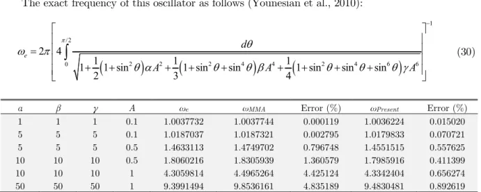
The exact frequency of this oscillator as follows (Younesian et al., 2010):
1
/2
2 2 2 4 4 2 4 6 6
0
2 4
1 1 1
1 1 sin 1 sin sin 1 sin sin sin
2 3 4
e
d
A A A
(30)A ωe ωMMA Error (%) ωPresent Error (%)
1 1 1 0.1 1.0037732 1.0037744 0.000119 1.0036224 0.015020 5 5 5 0.1 1.0187037 1.0187321 0.002795 1.0179833 0.070721 5 5 5 0.5 1.4633113 1.4749702 0.796748 1.4551515 0.557625 10 10 10 0.5 1.8060216 1.8305939 1.360579 1.7985916 0.411399 10 10 10 1 4.3059814 4.4965264 4.425124 4.3342404 0.656274 50 50 50 1 9.3991494 9.8536161 4.835189 9.4830481 0.892619
Table 1: A comparison between the natural frequencies with various parameters for Example 1.
Figure 3: A comparison between the approximate and exact solutions for Example 1, with = 50, = 100, = 100, A = 1.
3.2 Example 2
We consider the following nonlinear oscillator (He, 2002):
2
(1u )u u 0, u(0) A, u(0) 0 (31)
The linearized equation of Eq. (31) is:
2 0
u u (32)
The equation error between the two Eqs. (31) and (32) is:
2 2 2 2
( ) (1 )
e u u u u u uu u u u (33)
where ω2 is determined by using the mean-square criterion, as follows:
2 3
2
2
u u u
u
(34)
The periodic solution of linearized Eq. (32) is:
( ) cos( )
u t A t (35)
Using the definition (14), we calculate averaging operators in Eq. (34):
2 2 2 2 2 2 2
0
4 2
2 2 2 2
0 2 2
os cos ( )
2 8 ( ) ( 4 s ) co s t s
u A c t A s te t dt
s s
A s e d
s A
(36)4 2 6 8
2 2 2
3 4 2 4 4 2 2 2 4
0
4 2 2 4 4 2
0 2
248 416 1536 28 ( 4)
os cos ( )
co
( 16) s ( )
s t
s s s s s
s s
u u A c t A s te t dt
A s e d A
(37)With s is chosen equal to 2, substituting Eqs. (36) and (37) into Eq. (34), we get:
2 1 2 9216 2
12800
A
(38)2
1 1 0.72 A
(39)
And thus, the approximate solution of this oscillator is:
2 1 ( ) cos
1 0.72
u t A t
A
(40)
To illustrate the remarkable accuracy of the obtained results, we compare the approximate pe-riod
2
2 1 0.72
T A (41)
with the approximate period abtained by Modified Lindstedt-Poincare method (MLPM) (He, 2002)
2
3 2 1
4
MLPM
T A (42)
and the exact one (He, 1999)
2 2
0 4
ln(1 ) ln(1 )
A
ex
du T
A u
(43)In case A2 , Eq. (43) reduces to (He, 2002):
2
lim ex 2 2
A
T A
(44)So for large ε, it follows:
ex
T
A
(45)It is obvious that the approximate periods (41) and (42) have the same feature as the exact one
for
1
. And in case
, we have2 2
lim
0.9403
2 0.72
ex
A
T
A
T
A
(46)2 2
lim
0.9213
3
ex
A
MLPM
T
A
T
A
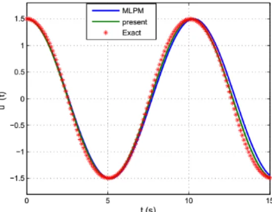
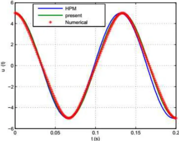
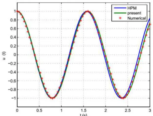
(47)Figure 5: Comparison of time history diagram of displacement between the Present, MLPM and Exact solutions at ε=5, A=1.
Figure 6: Comparison of time history diagram of displacement between the Present, MLPM and Exact solutions at ε=1, A=1.5.
Therefore, for any values of ε, it can be easily proved that the maximal relative error is less
than 6.349% for this method and 8.54% for Modified Lindstedt-Poincare method on the whole solu-tion domain (
0
).The numerical results obtained by three different methods are illustrated in Figs. 5-6 for
differ-ent values of ε and A. Numerical results validate the gain accuracy of this method.
3.3 Example 3
We consider the following nonlinear oscillator (Darvishia et al., 2008; Lim et al., 2006):
3
2 0, (0) , (0) 0
1 u
u u A u
u
(48)
2 3
(1u )uu 0 (49)
The linearized equation of Eq. (49) is:
2 0
u u (50)
The equation error between the two Eqs. (49) and (50) is:
2 3 2 2 3 2
( ) (1 )
e u u uu u uu uu u (51)
where ω2is determined by using the mean-square criterion, as follows:
3 4
2
2
uu u
u
(52)
The periodic solution of linearized Eq. (50) is:
( ) cos( )
u t A t (53)
Using the solution (53), we calculate averaging operators in Eq. (52), then substituting these
operators into Eq. (52) and with note that parameter s is chosen equal to 2, we get the approximate
frequency of this oscillator:
2
2 0.72 1 0.72
A
A
(54)
Thus, the approximate solution of this oscillator is:
2 2
0.72 ( ) cos
1 0.72 A
u t A t
A
(55)
A ωex ωPEM R. Error (%) ωPresent R. Error (%)
0.01 0.00847 0.00866 2.24321 0.00848 0.11806 0.05 0.04232 0.04326 2.22117 0.04239 0.16541 0.1 0.08439 0.08628 2.23960 0.08455 0.18959 0.5 0.38737 0.39736 2.57893 0.39057 0.82608 1 0.63678 0.65465 2.80631 0.64699 1.60338 5 0.96698 0.97435 0.76217 0.97333 0.65668 10 0.99092 0.99339 0.24926 0.99313 0.22303
Table 2: Comparison of the approximate frequencies with the exact frequencies.
Comparison of the approximate frequencies ω in Eq. (54) and the approximate frequencies
ob-tained by Parameter-Expansion Method (PEM) ωPEM (Bayat et al., 2012) in Eq. (56) with exact
frequencies ωex in Eq. (57) is tabulated in Table 2. Table 2 shows that the maximum relative error
2
2 3 4 3
PEM
A
A
(56)
Figure 7: Comparison of time history diagram of displacement between the Present, PEM and Exact solutions at A=0.1.
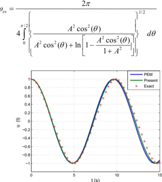
The exact frequency of this oscillator is (Ganji et al., 2010):
1/2
/2 2 2
2 2
2 2
0
2
2
cos ( ) 4
cos ( ) cos ( ) ln 1
1
ex
A
d A
A
A
(57)Figure 8: Comparison of time history diagram of displacement between the Present, PEM and Exact solutions at A=1.
The accuracy of the solution obtained this method can be observed in Figs. 7-8 which represent
comparisons of analytic solutions of u(t) based on time for this method and the one obtained by
3.4 Example 4
We consider the Duffing oscillator with discontinuity (He, 2004a):
3
0
u
u
u u
(58)with the initial conditions:
(0) , (0) 0
u A u (59)
The linearized equation of Eq. (58) is:
0
u
u
(60)The equation error between the two Eqs. (58) and (60) is:
3
( )
e u u u u u (61)
The unknown coefficient is determined from the mean square error criterion
2( ) 0
e u
it follows that:
4 2
2
u u u
u
(62)
The priodic solution and the frequency of Eq. (60) are:
( ) cos( ),
u t
A
t
(63)It is similar to Example 1, Example 2 and Example 3, we calculate averaging operators
u
2 ,2
u u
andu
4 ; and then substituting these operators into Eq. (62), yields the approximatefre-quency:
2
0.8324
A
0.72
A
(64)and the approximate solution:
2
( ) cos 0.8324 0.72
u t A A A t (65)
Accuracy of the approach for this example is shown in Figs. 9–11. We performed a comparison between the results obtained by this method, the ones obtained by He (He, 2004a) using the
Ho-motopy Perturbation Method and outcomes achieved using Runge-Kutta 4th order for different
Figs. 9-11, with the small, middle and large values of and ε, show that the results obtained by the present method are more exact than the ones obtained by the homotopy perturbation method.
We compare the approximate period obtained by this method T with the one obtained by the
Homotopy Perturbation Method THPM .
The approximate period of this oscillator is:
2
2
0.8324
0.72
T
A
A
(66)The approximate period obtained by the Homotopy Perturbation Method (He, 2004a) is:
2 2
8 3
3 4
HPM
T
A A
(67)
In case ε=0, these periods can be written as:
1/2 1 2
2
7.405
0.72
T
A
A
(68)and
1/2 1 2
4
7.255
3
HPM
T
A
A
(69)The exact period can be readily obtained, which reads (Acton et al., 1985):
1/ 2 1
7.416
e x
T A (70)
Thus, the maximal relative error of THMP is less than 2.2% and the maximal relative error of T
is less than 0.15% for all >0.
Figure 10: A comparison between the approximate and Runge–Kutta solutions for Example 3, = 3, ε = 1, A = 0.6.
Figure 11: A comparison between the approximate and Runge–Kutta solutions for Example 3, = 3, ε = 1, A = 1.
4 CONCLUSIONS
In this paper, the equivalent linearization method with weighted averaging is applied to analyze the nonlinear oscillation systems. This method is proposed by Anh in 2015. The accuracy of this meth-od is investigated by four nonlinear oscillation systems. The results show that this methmeth-od is useful to obtain analytical solutions for oscillators and vibration problems with nonlinearities. And the results indicate that the solution procedure is easy and provide a remarkable accuracy. However,
the value of the parameter s in the express of weighted coefficient h(t) should be chosen to give
better and the best solution is still required further investigation.
Acknowledgements
This research is funded by Vietnam National Foundation for Science and Technology Development
References
Alireza Khatami Jouybari and Mohamad Ramzani. Analytical methods for solving nonlinear motion of simple pendu-lum attached to a rotating rigid frame. International Journal of Mechatronics, Electrical and Computer Technology. Vol. 4(10), Jan, 2014, pp. 11-22.
Anh, N. D. Short Communication Dual approach to averaged values of functions: a form for weighting coefficient. Vietnam Journal of Mechanics.Vol. 37, No. 2 pp. 145 – 150 (2015).
Anh, N.D., Di Paola, M. Some extensions of Gaussian equivalent linearization. Proceedings of the International Con-ference on Nonlinear Stochastic Dynamics. pp. 5–16. Hanoi, Vietnam (1995).
Anh, N.D., Schiehlen, W. New criterion for Gaussian equivalent linearization. Eur. J. Mech. A/Solids. 16, 1025–1039 (1997).
C.W. Lim, B.S. Wu, W.P. Sun. Short Communication: Higher accuracy analytical approximations to the Duffing-harmonic oscillator. Journal of Sound and Vibration. 296 (2006) 1039–1045.
Caughey, T. K. Equivalent linearization technique. J. Acoust. Soc. Am.35, 1706–1711 (1959).
Davood Younesian, Hassan Askari, Zia Saadatnia, Mohammad KalamiYazdi. Frequency analysis of strongly nonline-ar generalized Duffing oscillators using He's frequency-amplitude formulation and He's energy balance method. Com-puters and Mathematics with Applications. 59 (2010) 3222-3228.
Elishakoff I, Andriamasy L, Dolley M. Application and extension of the stochastic linearization by Anh and Di Pao-la. Acta Mechanica. 204:89-98 (2009).
Guo-hua Chen, Zhao-Ling Tao, Jin-Zhong Min. Notes on a conservative nonlinear oscillator. Computers and Mathe-matics with Applications. 61 (2011) 2120–2122.
H. Ebrahimi Khah, D. D. Ganji. A Study on the Motion of a Rigid Rod Rocking Back and Cubic-Quintic Duffing Oscillators by Using He’s Energy Balance Method. International Journal of Nonlinear Science. 10(2010) No.4,pp.447-451.
Iman Pakar, Mahmoud Bayat and Mahdi Bayat. Analytical evaluation of the nonlinear vibration of a solid circular sector object. International Journal of the Physical Sciences. 6(30), pp. 6861 - 6866, 2011.
Iyengar, R. N. Higher order linearization in nonlinear random vibration. Int. J. Non-Linear Mech. 23, 385–391 (1988).
J.-H. He. Asymptotology by homotopy perturbation method. Applied Mathematics and Computation. 156 (2004b) 591–596.
J.H. He. Homotopy perturbation technique. Comput. Methods Appl. Mech. Engrg. 178 (1999) 257-262. J.R. Acton, P.T. Squire. Solving Equations with Physical Understanding, Adam Hilger Ltd, Bristol, 1985.
Ji-Huan He. Comparison of homotopy perturbation method and homotopy analysis method. Applied Mathematics and Computation. 156 (2004c) 527–539.
Ji-Huan He. Max-Min Approach to Nonlinear Oscillators. International Journal of Nonlinear Sciences and Numerical Simulation. 9(2),207-210,2008.
Ji-Huan He. Modified Lindstedt-Poincare methods for some strongly non-linear oscillations Part I: expansion of a constant. International Journal of Non-Linear Mechanics. 37 (2002) 309-314.
Ji-Huan He. The homotopy perturbation method for nonlinear oscillators with discontinuities. Applied Mathematics and Computation. 151 (2004a) 287–292.
Krylov N, Bogoliubov N. Introduction to nonlinear mechanics. New York: Princenton University Press, 1943. M. Kalami Yazdi, H. Ahmadian, A. Mirzabeigy, and A. Yildirim. Dynamic Analysis of Vibrating Systems with Non-linearities. Commun. Theor. Phys. 57 (2012) 183–187.
M.T. Darvishia, A. Karami, Byeong-Chun Shin. Application of He’s parameter-expansion method for oscillators with smooth odd nonlinearities. Physics Letters A. 372 (2008) 5381–5384.
Mahmoud Bayat, Iman Pakar, Ganji Domairry. Recent developments of some asymptotic methods and their applica-tions for nonlinear vibration equaapplica-tions in engineering problems: A review. Latin American Journal of Solids and Structures. 9(2012) 145-234.
S. Ghafoori, M. Motevalli, M.G. Nejad, F. Shakeri, D.D. Ganji, M. Jalaal. Efficiency of differential transformation method for nonlinear oscillation:Comparison with HPM and VIM. Current Applied Physics. 11 (2011) 965-971. S.S. Ganji, D.D. Ganji, A.G. Davodi, S. Karimpour. Analytical solution to nonlinear oscillation system of the motion of a rigid rod rocking back using max–min approach. Applied Mathematical Modelling. 34 (2010) 2676–2684.
S.S. Ganji·D.D. Ganji·Z.Z. Ganji·S. Karimpour. Periodic Solution for Strongly Nonlinear Vibration Systems by He’s Energy Balance Method. Acta Appl Math. (2009) 106: 79–92.
Seher Durmaz, Sezgin Altay Demirbağ, Metin Orhan Kaya. Approximate solutions for nonlinear oscillation of a mass attached to a stretched elastic wire. Computers and Mathematics with Applications. 61 (2011) 578–585.
Shahram Shahlaei-Far, Airton Nabarrete and José Manoel Balthazar. Nonlinear Vibrations of Cantilever Timoshenko Beams: A Homotopy Analysis. Latin American Journal of Solids and Structures. Vol. 13, Nr.10 (2016) 1866-1877. Turgut O¨ zis, Ahmet Yıldırım. A note on He’s homotopy perturbation method for van der Pol oscillator with very strong nonlinearity. Chaos, Solitons and Fractals. 34(2007) 989–991.