Estimation of age at death from the pubic symphysis and the auricular surface of the ilium using a smoothing procedure

Elsevier Editorial System(tm) for Forensic Science International Manuscript Draft

Manuscript Number: FSI-D-10-00324R3

Title: Estimation of age at death from the pubic symphysis and the auricular surface of the ilium using a smoothing procedure

Article Type: Original Research Paper

Keywords: age estimation, bone indicators, empirical bayes, human aging variability, density estimation, kernel estimation

Corresponding Author: Mr. Rui Costa Martins, M.D.

Corresponding Author's Institution: Escola Superior de Saúde Egas Moniz First Author: Rui C Martins, M.D.

Order of Authors: Rui C Martins, M.D.; Paulo E Oliveira, Ph.D.; Aurore Schmitt, Ph.D.

Abstract: We discuss here the estimation of age at death from two indicators (pubic symphysis and the sacro-pelvic surface of the ilium) based on four different osteological series from Portugal, Great-Britain, South Africa or USA (European origin). These samples and the scoring system of the two indicators were used by Schmitt et al. (2002), applying the methodology proposed by Lucy et al.

(1996). In the present work, the same data was processed using a modification of the empirical method proposed by Lucy et al. (2002). The various probability distributions are estimated from training data by using kernel density procedures and Jackknife methodology. Bayes's theorem is then used to produce the posterior distribution from which point and interval estimates may be made. This statistical approach reduces the bias of the estimates to less than 70% of what was obtained by the initial method. This reduction going up to 52% if knowledge of sex of the individual is available, and produces an age for all the individuals that improves age at death assessment.

* Corresponding author : tel: +351 965054893; fax: +351212946832 Email address: ruuimartins@ymail.com

Estimation of age at death from the pubic symphysis and the auricular surface of the ilium using a smoothing procedure

Rui Martins1*_{, Paulo Eduardo Oliveira}2

, Aurore Schmitt3

1

ruimartins@ymail.com

Centro de Investigação Interdisciplinar Egas Moniz (ciiEM), Escola Superior de Saúde Egas Moniz (ESSEM), Quinta da Granja, Monte de Caparica, 2829-511 Caparica - Portugal

and

Centro de Estatística e Aplicações da Universidade de Lisboa (CEAUL), Faculdade de Ciências da Universidade de Lisboa, Bloco C6 - Piso 4, Campo Grande, 1749-016 Lisboa – Portugal

2

paulo@mat.uc.pt

CMUC, Department of Mathematics, University of Coimbra, Portugal, Apartado 3008, 3001-454 Coimbra – Portugal

3

aurore.schmitt@univmed.fr

CNRS, UMR 6578- Anthropologie bioculturelle, Faculté de Médecine - Secteur Nord, Université de la Méditerranée, CS80011, Bd Pierre Dramard, 13 344 Marseille Cedex 15- France

Estimation of age at death from the pubic symphysis and the auricular surface of the ilium using a smoothing procedure

Abstract

We discuss here the estimation of age at death from two indicators (pubic symphysis and the sacro-pelvic surface of the ilium) based on four different osteological series from Portugal, Great-Britain, South Africa or USA (European origin). These samples and the scoring system of the two indicators were used by Schmitt et al. (2002), applying the methodology proposed by Lucy et al. (1996). In the present work, the same data was processed using a modification of the empirical method proposed by Lucy et al. (2002). The various probability distributions are estimated from training data by using kernel density procedures and Jackknife methodology. Bayes's theorem is then used to produce the posterior distribution from which point and interval estimates may be made. This statistical approach reduces the bias of the estimates to less than 70% of what was obtained by the initial method. This reduction going up to 52% if knowledge of sex of the individual is available, and produces an age for all the individuals that improves age at death assessment.

Keywords: age estimation, bone indicators, empirical bayes, human aging variability, density estimation, kernel estimation

1 Introduction

Estimation of age at death is a prerequisite for forensic identification and paleoanthropological studies. Research on estimation methods for the age of adult skeletons is still a developing area in both fields. It is now well established that inter-individual variability of age-related bone changes are caused by a complex interaction between many factors, and that the observed pattern may be different depending on the population under study [1-8].

Many calibration procedures have been proposed, but the majority of them give young individuals an age higher than they actually are and older individuals an age lower than real one. The most used methods include simple linear regression, multiple linear regression [9], classical calibration [10], methods based on analysis of nearest neighbours [11], inverse linear calibration, nonlinear inverse calibration, curvilinear regression [12] and Bayesian approaches [13-14]. This latter approach is not entirely new, having already appeared in a somewhat different framework, in the literature on fisheries, with the name of ``age length key''. In recent years Bayesian approaches have improved significantly, due to increased computer power which made more efective the calculation of posterior distributions. A very detailed description of these and other methods can be found in several papers [15-20].

However, due to difficulties associated with the complex variety of aging processes and the problems resulting from the methodology used to classify changes in the human skeleton, estimation of age at death is not always as precise as it should. The increasing number of methods published every year based on teeth or bone indicators, reflects the difficulty of reaching accurate and reliable estimates [21]. Most of the methods applied are based on the visual scoring of morphological indicators of age, such as degenerative changes of articular joint surfaces. The simplicity and rapidity of a method make it a useful tool for quick evaluation of indicators and cheap estimation in forensic and archaeological context. Pubic symphysis and auricular surface of the ilium have been largely exploited to create methods, but these were based on observations of *Manuscript (without author identifiers)

a single population [22-26]. One of authors has tested her method based on a worldwide learning sample [27] using a Bayesian prediction approach in order to classify individuals in age range categories. The results show that combination of the pubic symphysis and the auricular surface of the ilium do not perform better than the auricular surface used as a single indicator. Bayesian prediction produced reliable, though not very precise, classification and produced approximations also for subjects over 50 years old, which is a real methodological improvement when compared to others methods. As the European series show the same trend of variation, it was proposed in further publications to aggregate European series in order to take into account the largest variability on both indicators treated separately [28-29].

The present work proposes to use the samples and the scoring system suggested by Schmitt [27-29] using another statistical treatment in order to improve age at death assessment.

2 Material

The observed material comes from four different osteological series. Two European collections from documented cemeteries were studied: Conchada Cemetery, Coimbra, Portugal [30]; Spitalfields Cemetery, London, Great Britain [31]. We observed individuals from European origins of the Hammann-Todd collection, Cleveland, USA [32] and subjects with an African origin of the Dart collection, Johannesburg, South-Africa. The number of individuals in each collection according to sex are presented in Table 1. In order to keep anthropological meaning the global sample was chosen so that age distribution between age intervals is homogeneous.

3 Methods

3.1 Scoring system

Here we present a brief summary of the scoring system used to estimate the age at death. This system aims to reduce errors between different observers, as similarity between the classifications assigned by two observers for the same individual are of order 90% [33].

The observation of the two indicators - pubic symphysis area and the sacro-pelvic surface of the ilium - is based on anatomical criteria. Four features on the sacro-pelvic surface of the ilium (SPI) are observed: transverse organization (SPIA - two phases), modification of the articular surface (SPIB - four phases), modification of the apex (SPIC - two phases), and modification of the iliac tuberosity (SPID - two phases). Three features are examined on the pubic symphysis (SPU): posterior plate (SPUA - three phases), anterior plate (SPUB - three phases), and posterior lip (SPUC - two phases). This makes a scoring system that has 576 different classification classes. The new scoring system is fully described, with illustrations, in Schmitt [28-29].

3.2 Statistical methodologies

The methodology used is based on a Bayesian decomposition with a kernel smoothing for estimation, following the approach in Lucy et al. [19]. We present a brief description of the theoretical relations between the various functions. If X is the variable representing age and we have m indicators Y=



Y₁,Y₂,,Y_m



, the posterior distribution for age given conditional on the indicators is, according to Bayes theorem







_{ }



y y y f x f x f x f | = | ( ) (1)

where y=



y₁,,y_m



and f



y|x



is a m-dimensional joint likelihood of the indicators given X and f(x) is the prior distribution for X . The marginal density function f

 

y , can be found by integrating with respect to age the numerator on the right.

Characterizing the joint likelihood f



y|x



is trickier, as it depends on the relations between variables and within indicators. A first approach assumes conditional independence between Y_i's given X . So, the likelihood in equation (1) can be written as:



|



= ( | ) 1 = x y f x f i m i



y (2)

where f(yi|x) is the individual univariate conditional distribution of Yi given X . If full

conditional independence is not a reasonable assumption, one may use the partial independence method proposed by Chow and Liu [34]. This reduces to constructing a dependence tree by searching the highest correlations between variables. A dependence tree describes a path among the variables that proceeds by connecting at each step the highest correlated variables. The algorithm to achieve this is as follows: compute the correlation for all pairs of variables involved; add a branch between the two variables with highest absolute correlation value, then a branch between the two variables whose correlation has the second largest absolute value ignoring those that create cycles, and so on; after all branches have been found, stop and arbitrarily choose one of the variables as a starting point. In this way, except for the root, each variable may be thought of as descending from another one. For a given indicator i , denote by j(i) it parent in this relation. This function j() is called the dependence tree. Then, the joint likelihood is written as the product of m1 pairwise conditional probabilities distributions:



x



f



y y x



f i j i m i , | = | () 1 =



y (3)

where m is the number of variables, yj(i) is the parent of yi in a conditional dependency tree,

whose root y is chosen arbitrarily and f



y|yj(),x



= f



y|x



,.

In order to obtain estimates fˆ of conditional and marginal densities we use the kernel method [35-36]. To estimate the density function f() of the univariate continuous variable X , this means computing:

R x h X x K h n x f n i n n i        



1 , 1 = ) ( ˆ 1 = (4) where hn is a positive sequence, limnhn =0, K(t)0 and



K( dtt) =1.

Using kernel methods means choosing a bandwidth h and a kernel function K , trying to minimize some error criterium. A variety of kernel functions have been used in the literature. Popular choices are the Epanechnikov kernel [37], and the standard Gaussian density, given its continuity, differentiability, and locality properties. A good discussion of kernel estimation techniques can be found in Wand and Jones [36].I. Anyway, it is well known that in practice any reasonable kernel produces nearly optimal results, so this choice is not determinant. On the other hand the choice of the bandwidth h is more sensitive. Silverman [35] proposes the following approach to the choice of the bandwidth when using a Gaussian kernel:



standarddeviation,interquartilerange/1.34



. min = , 0.9 = 5 1 A where An h  (5)

This choice is simple to evaluate and performs very well for a wide range of densities. A more accurate choice of the bandwith is the  level Plug-in direct rule proposed by Sheather and Jones [38] and described in Wand and Jones [36, p. 71]. The choice (5) is also a good starting point for this method.

Assuming age X to be a continuous variable while the indicators Y are considered discrete the bivariate kernel density estimator may be written as:

 

1





, = ) , ( ˆ 1 = i i n i y y h X x K y n y x f _       



 (6)

where K is a one-dimensional kernel with single bandwidth parameter h, (u) the indicator function     =1 1 if = 0 ( ) = = , 0 if 0 n i i u u and n y y y u  _    



is the number of observations equal to y . This corresponds to estimating a few conditional densities.

Lucy et al. [19] pointed out that smoothing between categorical variables does not make much sense and the kernel method could be inappropriate. So they use a smoothing technique suggested by Titterington [39]. However in many categorical models adjacency does means some kind of proximity, thus giving some reasonability to the application of smoothing techniques. This idea has been widely explored as in [40-49], for example. The scoring system introduced by Schmitt et al. [27] does show this proximity feature, thus giving justification to use of smoothing methods.

We decided to perform calculations for the different data using only SPU indicator (pubic symphysis), only SPI indicator (sacro-pelvic surface of the ilium) and both at same time, to verify which of the three scenarios produces better results. The morphological changes with aging are significantly different between the various populations. As a consequence, we decided to present first the results by population. These results are thus independent of each other and only apply to the population in particular. Our calculations also take into account the sex of each individual. Adopting a point of view more reasonable for the anthropological studies, as skeleton remains usually do not give information about a more specific origin, we also include results for pooled european populations, obtaining a model taking into account the european variability.

Calculations were carried out for each of the four groups of individuals and the european series pooled together, considering either dependence and conditional independence between the indicators given age. We opted to use the Gaussian kernel and a prior distribution based on the data. The bandwidth parameter, necessary in equation (4), is obtained through the direct plug-in rule [36, p. 71]. To assess the performance of the methodology we use a Jackknife approach (see Efron [50] for example), that is, we repeat the procedure: take one observation out and use the remaining observations as training sample to estimate the age at death of the left out observation. Of course, this means recomputing prior distributions and likelihood functions at each repetition of the process. Using this methodology seems to better reflect a real situation where the true ages are not known.

3.2.1 Example of an individual procedure

Here we illustrate the individual procedure used to compute the data for each skeleton with a 34 years old Portuguese female with the following values for the indicators

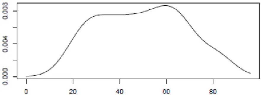
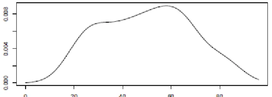
We exemplify only with the SPI indicator, but the two remaining cases, isolated SPU and SPU+SPI, are identical. The first step to estimate the age at death of the individual concerned is to estimate the various density functions needed to calculate equation (1) using the kernel method. In Figure 1 we show the approximation obtained using (4) for the prior distribution for the Portuguese population (males and females).

Figure 1

To compute the density function for age given the indicators, i.e. the likelihood, we use the methodology of Chow and Liu [34]. We describe this in detail next. Table 3 shows the empirical correlations between the various indicators.

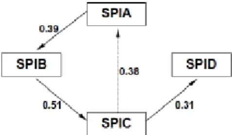
To build the dependency tree, choose the highest correlation, between SPIB and SPIC, and add a branch join them. The second highest correlation is between SPIA and SPIB, thus a branch connecting these is added. The following step would link SPIA to SPIC, but this would lead to a cycle, so it is ignored. The last link is SPIC - SPID. Now all the indicators are linked and any other branch that is added to the tree results in a cycle.

Figure 2

This tree, where the root was chosen arbitrarily, tells us that the appropriate form for equation (3) is ). age | SPIA ( ) age SPIA, | SPIB ( ) age SPIB, | SPIC ( ) age SPIC, | SPID ( = ) age | indicators ( f f f f f   

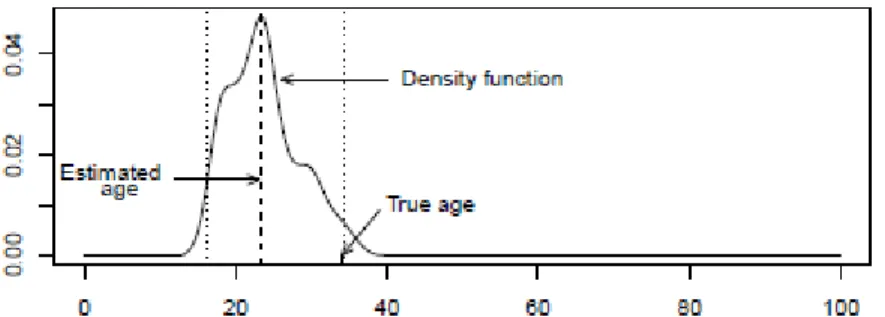
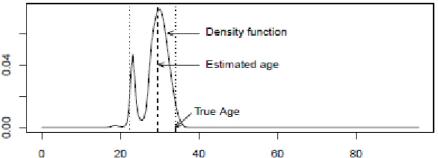
From the data we can compute estimates for the various distributions present in the previous equation. Once we have approximations for the prior density and the likelihood, we can use equation (1) to estimate the posterior distribution, which will enable us to estimate the age for each individual conditional on their indicators. Figure 3 below shows the posterior distribution for the considered individual.

Figure 3

Notice that this approximation for the posterior distribution holds for this given individual based on the learning sample considered here, which is the whole sample without the selected individual.

We now describe some conclusion that follow from the approximation constructed. The median of this distribution, which is an estimator for the age much more robust than the distribution mean, is 23.12, showing a discrepancy of about 11 years when compared to the true age (34 years). A 95% credible interval derived is simply the interval between 0.025 and 0.975 percentiles. For this example we obtain



14.57,34.17



, thus an interval with the range about 20 years. Do not forget that we are using all the Portuguese population to derive the prior distribution of the age and not only the Portuguese female population. Later on we present the results considering only the Portuguese female population.

In order to illustrate the effect of assumptions that influence the construction of the likelihood, consider now that the indicators are independent given age. Then the appropriate form for the likelihood is equation (2), which we can rewrite as:



indicators|age



=



i indicator|age



1 = 



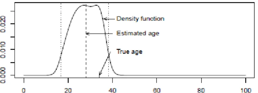
f f m i (7) In Figure 4 we can see the approximation that is now obtained for the posterior distribution for the age of the same individual that is being analysed.

Figure 4

The estimation parameters for the age is now 28.05, the median of the distribution, and the 95% credible interval is



16.6,38.28



.

It is now clear that the two situations produce very different results, as we shall see in Section 5. For this particular case the conditional independence of the indicators given age seems to produce better results.

3.2.2 Example of collective procedures

In the previous section we described how to estimate the age of an individual and find a 95% credible interval. The purpose of the present section is to show how to process global measures that enable us to compare the accuracy of the various estimates obtained and to analyze the results. The global measures used are:

1. MAD - the mean absolute deviation

| ˆ | 1 |= | 1 = 1 = 1 = i i n i i n i x x n e n MAD





 (8)

where x_i is the true age for the i -th individual and xˆi is the estimated age;

2. Bias - the slope,

2 = x xe s s  (9)

of the linear regression line of the residuals, e_i =x_ixˆ_i vs. the true age which is a measure of systematic bias.  >0 means that the age of the younger individuals is overestimated and the age of the older is underestimated;

3. Mean width - mean width of the 95% credible intervals;

4. Coverage - percentage of 95% credible intervals that contain the true age.

Remember that, as referred before, to assess the global performance of the methodology we use a Jackknife resampling approach: take one observation out and use the remaining observations as training sample to estimate the age at death of the left out observation. All graphs and calculations were carried using R. This statistical computing software that can be obtained at http://cran.r-project.org.

4 Results

In the analysis of the five sets of data, when it was supposed conditional independence between indicators and age, we tested the dependency tree in both directions, but the results were similar, with no major discrepancy. That is, considering root for either end of the tree, the results obtained for the age of several individuals were identical.

Looking at the results globally (Tables 4 to 8), it is clear that these are more accurate when we use the SPU and SPI indicators together. The intervals of smaller width are obtained when considering the conditional dependence between indicators given age and when we do not proceeded to smoothing discrete variables, as suggested by Titterington [39].

For example, using the Portuguese data set we obtained, considering partial independence and no smoothing of the discrete indicators, credible intervals with width of about 26 years, while for the British data set this width is around 31 years. The coverage is around 68% and 77%, respectively. The case of U.S. residents of European origin we obtained a width of about 29 and a coverage of 70%. The African seems to be the worst case. The results for the pooled data set agree with the above, that is, the smallest credible intervals correspond to assuming partial independence and no smoothing of discrete indicators. For this pooled data, the best width for the credible interval is around 31.5 years, thus just a little larger than the worst european population considered alone. The coverage is now 82%, which is not surprising. In fact, enlarging the credible interval means that the coverage for the subsamples that had produced smaller credible intervals is well increased.

Use of conditional independence together with smoothing of discrete variables seems to be the worst case, producing larger credible intervals. The African data set is again the one that produces the worst results.

The remaining sets, when analysed without taking into account the sex, show the level of accuracy that was reported by Lucy et al. [19] who did not take into account sex. However, when we take the sex of individuals into account, our results are improved, particularly with regard to the intervals width. The exception is, once again, the African population.

This methodology produces reasonable estimates for the age of younger individuals. For example, for the European pooled series the mean absolute deviation of the 25% youngest individuals in the sample is 9.17, while if you look for the 10% youngest the MAD is 5.42. Looking at specific population series generally improves on these results. Again, as an example, using the Portuguese series, the 25% youngest show a MAD equal to 6.33, while for the 10% youngest this reduces to just 1.65. These results are consistently better than the MAD values reported in Table 8. On the other hand, estimates for the age of older individuals continue to show very large differences with respect to the real age. In particular, the deviation from the estimated age for the older individual, for each data set, is systematically higher than the MAD. As illustrated before, using now the European pooled series, the MAD computed over the 25% oldest is11.67 and computed over the 10% oldest one still has 11.39, thus clearly above the overall values reported in Table 8.

If we look at results by sex using the two indicators together, we find that, the separate analysis of male individuals produces better results than the female data set with respect to the four measures of accuracy. In Section 3.3, we estimated the age of the female individual as about 23 years with a 95% credible interval



14.57,34.17



. After proceeding to the separation of the data set by sex, the estimate obtained for the age of this same individual it 29 years and a 95% credible interval



22.61,34.17



. Therefore, there was a significant improvement in results for the individual mentioned above. In Figure 5 we show the prior density function for the Portuguese women data without the inclusion of the individual cited and using both indicators. Figure 6 shows the posterior distribution that allowed us to obtained the estimates mentioned. Comparing with the posterior distribution obtained without the knowledge of sex, given in Figure 4, it is clear why the estimate of age for this individual is better than the one described earlier in Section 3.3.

Figures 5 and 6

5 Discussion

Credible intervals with smaller length were obtained when considering partial dependence between indicators and no smoothing of the discrete variables. In this case partial dependence can be interpreted as follows: knowing the age of a skeletal and the level of an indicator, e.g. SPUA, increases (or decreases) our belief in a particular level of another indicator, e.g. SPUB. If the indicators were in fact independent, knowledge of the age of a skeletal would be enough to increase (or decrease) our belief in a particular level of an indicator, while knowledge about another indicator would not add anything to our beliefs. For example, observing that the score for the indicator SPUA is 3 (even if the true age-at-death was 35 years old) causes us to increase our belief in SPUB being score 2 or 3 and decrease the belief in score 1. So the indicators are at least partial dependent. The results also show that smoothing is not a good idea. We think that this happens because for this scoring system indecision about the level of each indicator has a low probability. This should be the reason why this scoring system has a good performance. Kernel density methods for the estimation of probability density functions in age prediction increase accuracy because these procedures make no assumptions on the distributions, as is always implicit in parametric approaches. This methodology also seems to make better use of the available information in the data.

In the present work, a few results contradict those obtained by Schmitt et al. [27]. Notice that we are using the same samples, but a different statistical methodology. First, we conclude that usage of both indicators yields better results than using a single one. We mention that multifactor techniques are recommended by many authors [51-54] and criticized by others [33]. Secondly, when combined, the two indicators produce better results for the analysis of males than for females. The analysis of the African series shows that the credible intervals and the bias are much higher than for European samples. This result seems related to the fact that morphological differences with aging within the African sample are clearly different from the European population that exhibits a rather common trend of variation.

In all cases, the bias is quite large, which shows that we are overestimating the age at death for young people and underestimated to the age of the older. This issue remains one of the biggest obstacles to developing an effective method to estimate age at death, and a process that can overcome this problem is certainly in the right direction.

One significant advantage of the statistical methodology proposed here is that it allows to produce a credible age interval for all individuals, while the method used by Schmitt et al. [27] presents individuals who were not classified. This means that the procedures are more sensitive to uncertainties and more accurate. The parametric Bayesian model used [27] was unable to classify some individuals because it tries to assign an individual to a pre-specified interval (usually divided into decades).

It is also advisable, when possible, to perform analysis of the data taking into account the sex of the different individuals and using both indicators in the calibration, because the results we obtained appear to be substantially better.

6 Conclusion

The main goal of the present paper was to improve the method proposed by Schmitt [27] and Schmitt et al. [28, 29] to estimate the age at death based on measuring modifications of the

pubic symphysis and auricular surface of the ilium. This study has thus been carried over the same sample used before. The statistical approach used here is advantageous because, as reported above, it produces smaller credible intervals and improves the estimates obtained for younger individuals. Moreover, opposite to the previous approach, this methodology is able to provide age estimation for every individual. The results also indicate that sex information, whenever available, improves significantly the estimates. The same improvement is observed if we use both indicators instead of just one, as was indicated in Schmitt [27]. Nevertheless, the global reliability of this statistical approach remains close to what was obtained by the previous methodology, which was more or less expected given the variability of bone modifications with the aging process.

References

[1] M. Cox, Ageing adults from the skeleton, in: M. Cox, S. Mays (Eds), Human Osteology in Archeology and Forensic Science, London, Greenwich Medical Media, 2000, pp. 61-81

[2] D.H. Ubelaker, Methodological consideration in the forensic applications of human skeletal biology, in: M.A. Katzenberg, S.R. Saunders (Eds), Biological Anthropology of the Human Skeleton, New York, Wiley-Liss, 2000, pp. 41-67.

[3] M. Jackes, Building the bases for paleodemographic analysis : adult age determination, in: M.A. Katzenberg, S.R. Saunders (Eds), Biological Anthropology of the Human Skeleton, New York, Wiley-Liss, 2000, pp. 417-466.

[4] C.G. Falys, H.Schutkowski, D.A. Weston, Auricular surface aging: Worse than expected? A test of the revised method on a documented historic skeletal assemblage, Am. J. Phys. Anthropol. 130 (2006) 508-513.

[5] A. Meinl, C. D. Huber, Comparison of the validity of three dental methods for the estimation of age at death, Forensic Sci. Int. 178 (2008) 96-105.

[6] S.M. Hens, E. Rastelli, G. Belcastro, Age Estimation from the Human Os Coxa: A Test on a Documented Italian Collection, J. Forensic Sci. 53 (2008) 1040-1043.

[7] U. Wittwer-Backhofen, J. Buckberry, A. Czarnetzki, S. Doppler, G. Grupe, G. Hotz, A. Kemkes, C.S. Larsen, D. Prince, J. Wahl, A. Fabig, S. Weise, Basics in paleodemography: acomparison of age indicators applied to the early medieval skeletal sample of Lauchheim, Am. J. Phys. Anthropol. 137 (2008) 384-396.

[8] A. Schmitt, B. Saliba-Serre, M. Tremblay, L. Martrille, An Evaluation of Statistical Methods for the Determination of Age of Death Using Dental Root Translucency and Periodontosis, J. Forensic Sci. 55 (2010) 590-596.

[9] W.R Maple, An improved technique using dental histology for the estimation of adult age, J. Forensic Sci. 23 (1978) 764-770.

[10] L.W. Konisgberg, S.R. Frankenberg, Paleodemography: «Not quite dead», Evolution and Anthropology, 3 (1994) 92-105.

[11] D. Ferembach, I. Schwidetzky, M. Stloukal, Recommendations for age and sex diagnosis of skeletons, J. Hum. Evol. 9 (1980) 517-550.

[12] G. Bang, E. Ramm, Determination of age in humans from root dentine transparency, Acta Odontol. Scand. 28 (1970) 3-35.

[13] L.W. Konigsberg, S.R. Frankenberg, Estimation of age structure in anthropological demography, Am. J. Phys. Anthropol. 89 (1992) 235-256.

estimation from dental observations by Johanson’s age changes, J. Forensic Sci. 41 (1996) 189-194.

[15] D. Lucy, A.M. Pollard, C.A. Roberts, A comparison of three dental techniques for estimating age at death in humans, J. Archaeol. Sci. 22 (1995) 417-428.

[16] D. Lucy, A.M. Pollard, Further comments on the estimation of error associated with the Gustafson dental age estimation method, J. Forensic Sci. 40 (1995) 222-227.

[17] R.G. Aykroyd, D. Lucy, A.M. Pollard, C.A.Roberts, Nasty, Brutish but not necessarily short, J. Am. Ant. 64 (1999) 55-70.

[18] R.G. Aykroyd, D. Lucy, A.M. Pollard, T. Solheim, Technical Note: Regression Analysis in Adult Age Estimation, Am. J. Phys. Anthropol. 104 (1997) 259-265.

[19] D. Lucy, R.G. Aykroyd, A.M.Pollard, Nonparametric calibration for age estimation, Appl. Stat. 51(2002) 183-196.

[20] E.A. DiGangi, J.D. Bethard, E.H. Kimmerle, L.W. Konisberg, A new method for estimating age-at-death from the first rib, Am. J. Phys. Anthropol., 138 (2009) 164-174.

[21] F.W. Rosing, M. Graw, B. Marre, S. Ritz-Timme, M.A. Rothschild, K. Rotzscher, A. Schmeling, I. Schroder, G. Geserick, Recommendations for the forensic diagnosis of sex and age from skeletons, Homo 58 (2007) 75-89.

[22] C.O. Lovejoy, R.S. Meindl, T.R. Prysbeck, R.P. Mensforth, Chronological metamorphosis of the auricular surface of the ilium : a new method for the determination of adult skeletal age at death, Am. J. Phys. Anthropol. 68 (1985) 15-28.

[23] S. Brooks, J.M. Suchey, Skeletal age determination based on the os pubis : a comparison of the Acsádi-Nemeskeri and Suchey-Brooks methods, Hum. Evol. 5 (1990) 227-238.

[24] J.L. Buckberry, A. Chamberlain, Age Estimation from the auricular surface of the ilium : a revised method”, Am. J. Phys. Anthropol. 119 (2002) 231-329.

[25] Y. Igarashi, U. Kagumi, W. Tetsuaki, E. Kanazawa, New method for estimation of adult skeletal age at death from the morphology of the auricular surface of the ilium, Am. J. Phys. Anthropol. 128 (2005) 324-339.

[26] X. Chen, Z. Zhang, L. Tao, Determination of male age at death in Chinese Han population: using quantitative variables statistical analysis from pubic bones, Forensic Sci. Int. 175 (2007) 36-43.

[27] A. Schmitt, P. Murail, E. Cunha, D. Rougé, Variability of the pattern of aging on the human skeleton: evidence from bone indicators and implications on age at death estimation, J. Forensic Sci. 47 (2002) 1-7.

[28] A. Schmitt, Une nouvelle méthode pour estimer l’âge au décès des adultes à partir de la surface sacro-pelvienne iliaque, Bulletins et Mémoires de la Société d’Anthropologie de Paris 17 (2005) 89-101.

[29] A. Schmitt, Une nouvelle méthode pour estimer l’âge des individus décédés avant et après 40 ans, Journal de Médecine Légale et de Droit Médical 51 (2008) 17-24.

[30] M.A. Rocha, Les collections ostéologiques humaines identifiées du Musée Anthropologique de l’Université de Coimbra, Antrop. Port. 13 (1995) 7-38.

[31] T. Molleson, M. Cox, The Spitalfields project volume 2-Anthropology, CBA Research Report, 86 (1993) 167-179.

[32] R.P. Mensforth, B.M. Latimer, Hamann-Todd Collection aging studies: osteoporosis fracture syndrome, Am. J. Phys. Anthrop. 80 (1989) 461-479.

[33] A.Schmitt, Variabilité de la sénescence du squelette humain. Réflexions sur les indicateurs de l’âge au décès: à la recherché d’un outil performant [dissertation]. PhD thesis, University of Bordeaux, 2001.

[34] C.K. Chow, C.N. Liu, Approximating Discrete Probability Distributions with Dependence Trees, IEEE Trans. Inf. Theory 14 (1968) 462-467.

[35] B.W. Silverman, Density estimation for statistics and data Analysis, Chapman and Hall, 1986.

[36] M.P. Wand, M.C. Jones, Kernel Smoothing, London, Chapman and Hall, 1995.

[37] V.A. Epanechnikov, Nonparametric estimation of a multidimensional probability density, Theory of Probability and its Applications 14 (1969) 153-158.

[38] S. J. Sheather, M. C. Jones, A reliable data-based bandwidth selection method for kernel density estimation, J. R. Stat. Soc. Series B. 53 (1991) 683–690.

[39] D.M. Titterington, A comparative study of kernel-based density estimates for categorical data, Technometrics 22 (1980) 259-268.

[40] J. Simonoff, A penalty function approach to smoothing large sparse contingency tables, Ann. Statist. 11 (1983) 208-218.

[41] J. Simonoff, Smoothing categorical data, J. Statist. Plann. Inference 47 (1995) 41-69. [42] J. Simonoff, Smoothing methods in statistics, Springer-Verlag, New York, 1996. [43] P. Burman, Smoothing sparse contingency tables, Sankhya, Ser. A 49 (1987) 24-36.

[44] P. Hall and D. Titterington, On smoothing sparse multinomial data, Austral. J. Statist. 29 (1987) 19-37.

[45] J. Dong and J. Simonoff, A geometric combination estimator for d-dimensional ordinal contingency tables, Ann. Statist. 23 (1995) 1143-1153.

[46] M. Aerts, I. Augustyns, and P. Janssen, Local polynomial estimation of contingency table cell probabilities, Statistics 30 (1997) 127-148.

[47] M. Aerts, I. Augustyns, and P. Janssen, Sparse consistency and smoothing for multinomial data, Statist. Probab. Lett. 33 (1997) 41-48.

[48] M. Aerts, I. Augustyns, and P. Janssen, Central limit theorem for the total squared error of local polynomial estimators of cell probabilities, J. Statist. Plann. Inference 91 (2000) 181-193. [49] P. Jacob, P.E. Oliveira, Relative smoothing of discrete distributions with sparse observations, J. Stat. Comput. Simul. 81 (2011) 109-121.

[50] B. Efron, The Jackknife, the Bootstrap, and Other Resampling Plans, Society for Industrial and Applied Mathematics, 1982.

[51] M.Y. Iscan, S. Loth, Osteological manifestation of age in the adult, in: M.Y. Iscan, K.A. Kennedy (Eds), Reconstruction of life from the Skeleton, New-York, Wiley-Liss, 1989, pp. 23-40.

[52] M.E. Bedford, K.F. Russel, C.O. Lovejoy, R.S. Meindl, S.W. Simpson, P.L. Stuart-Macadam, Test of the multifactorial aging method using skeletons with known ages-at-death from the Grant Collection, Am. J. Phys. Anthrop. 91 (1993) 287-297.

[53] R.S. Meindl, K.F. Russel, Recent advances in method and theory in paleodemography, Annu. Rev. Anthropol. 27 (1997) 375-399.

[54] E. Baccino, A. Schmitt, Determination of adult age at death in forensic context, in: A. Schmitt, E. Cunha, J. Pinheiro (Eds), Forensic Medicine and Anthropology. Two complementary Sciences. From recovery to cause of death, Totowa, Humana Press, 2006, pp. 259-280.

List and Legends of tables and figures

Table 1: Osteological samples used in the study.

Table 2: Bone indicator classifications for the 34 year old Portuguese Female. Table 3: Partial correlations between the indicators computed from the sample.

Table 4: Results of the African data. Aggregate computes estimates using the complete sample, Female or Male computes estimates using only individuals from the sample with same sex. MAD is the mean absolute deviation. Bias describes the regression slope of the residuals. Mean width describes the width of 95% credible intervals. Coverage computes the proportion of credible intervals that include the true age.

Table 5: Results of the Great-Britain data. Aggregate computes estimates using the complete sample, Female or Male computes estimates using only individuals from the sample with same sex. MAD is the mean absolute deviation. Bias describes the regression slope of the residuals. Mean width describes the width of 95% credible intervals. Coverage computes the proportion of credible intervals that include the true age.

Table 6: Results of the Portuguese data. Results of the Great-Britain data. Aggregate computes estimates using the complete sample, Female or Male computes estimates using only individuals from the sample with same sex. MAD is the mean absolute deviation. Bias describes the regression slope of the residuals. Mean width describes the width of 95% credible intervals. Coverage computes the proportion of credible intervals that include the true age.

Table 7: Results of the USA data. Aggregate computes estimates using the complete sample, Female or Male computes estimates using only individuals from the sample with same sex. MAD is the mean absolute deviation. Bias describes the regression slope of the residuals. Mean width describes the width of 95% credible intervals. Coverage computes the proportion of credible intervals that include the true age.

Table 8: Results of the european series pooled together. Aggregate computes estimates using the complete sample, Female or Male computes estimates using only individuals from the sample with same sex. MAD is the mean absolute deviation. Bias describes the regression slope of the residuals. Mean width describes the width of 95% credible intervals. Coverage computes the proportion of credible intervals that include the true age.

Figure 1: Prior density function for the age of the Portuguese population. Horizontal axis represents age in years.

Figure 2: Dependence tree to obtain the likelihood.

Figure 3: Posterior distribution for the 34 years old Portuguese female and assuming conditional dependence between indicators and age. Horizontal axis represents age in years.

Figure 4: Posterior distribution subsequent to the individual of 34 years considering the independence between indicators given age. Horizontal axis represents age in years.

Figure 5: Prior density function for the Portuguese women data set using both indicators. Horizontal axis represents age in years.

Figure 6: Posterior density function for the 34 years old woman calculated using only the female individuals and using both indicators. Horizontal axis represents age in years.

Figure 1: Prior density function for the age of the Portuguese population. Horizontal axis represents age in years.

Figure 3: Posterior distribution for the 34 years old Portuguese female and assuming conditional dependence between indicators and age. Horizontal axis represents age in years.

Figure 4: Posterior distribution subsequent to the individual of 34 years considering the independence between indicators given age. Horizontal axis represents age in years.

Figure 5: Posterior density function for the 34 years old woman calculated using only the female individuals and using both indicators. Horizontal axis represents age in years.

Figure 6: Posterior density function for the 34 years old woman calculated using only the female individuals and using both indicators.

Geographical Area Male Female Total

Portugal 39 51 90

South Africa (Soto and Zulu) 60 60 120

Great-Britain 46 50 96

U.S.A. (European origin) 58 62 120 Table 1

Age Sex SPUA SPUB SPUC SPIA SPIB SPIC SPID

34 female 2 2 1 2 1 2 1

SPIA SPIB SPIC SPID SPIA 1 0.39 0.38 0.16 SPIB 1 0.51 0.22 SPIC 1 0.31 SPID 1 Table 3

MAD Bias Mean width Coverage

Calibration SPU SPI

SPU + SPU SPI SPU + SPU SPI SPU + SPU SPI SPU +

method SPI SPI SPI SPI

Ag g re g a te Cond. Dep. Smoothing 13.65 14.87 13.61 0.77 0.74 0.6 59.14 53.47 48.57 0.92 0.90 0.86 No smoothing 13.46 14.85 13.29 0.67 0.68 0.54 56.20 47.88 44.25 0.88 0.84 0.77 Cond. Indep. Smoothing 14.68 13.77 13.62 0.97 0.88 0.87 65.81 64.64 62.56 0.97 0.97 0.97 No smoothing 12.84 13.79 12.31 0.74 0.75 0.61 61.76 57.60 52.35 0.94 0.92 0.89 F ema le Cond. Dep. Smoothing 14.37 16.55 15.53 0.73 0.81 0.65 58.77 55.75 52.43 0.92 0.89 0.85 No smoothing 15.57 17.26 15.65 0.61 0.82 0.60 57.15 50.93 46.33 0.89 0.82 0.79 Cond. Indep. Smoothing 14.91 14.68 14.24 0.95 0.94 0.90 69.46 70.71 67.87 0.97 0.97 0.97 No smoothing 13.52 15.69 14.31 0.76 0.85 0.72 63.45 64.15 55.98 0.94 0.95 0.87 M a le Cond. Dep.. Smoothing 12.58 14.70 13.25 0.72 0.68 0.53 59.94 49.30 45.84 0.91 0.88 0.86 No smoothing 12.61 14.99 13.55 0.68 0.64 0.44 55.79 41.02 33.89 0.84 0.71 0.72 Cond. Indep. Smoothing 15.45 13.10 13.48 1.00 0.84 0.85 64.94 62.64 60.48 0.97 0.97 0.97 No smoothing 12.46 13.53 11.91 0.73 0.70 0.55 57.77 52.36 45.06 0.91 0.84 0.81 Table 4

MAD Bias Mean width Coverage

Calibration SPU SPI

SPU

+ SPU SPI SPU+ SPU SPI

SPU

+ SPU SPI SPU+

method SPI SPI SPI SPI

Ag g re g a te Cond. Dep. Smoothing 13.64 10.08 10.01 0.80 0.37 0.52 51.09 43.87 41.91 0.88 0.88 0.86 No smoothing 13.50 10.42 10.99 0.73 0.26 0.31 53.97 31.29 31.20 0.91 0.75 0.77 Cond. Indep. Smoothing 16.01 12.43 12.4 1.00 0.77 0.77 69.88 71.01 67.83 0.97 0.97 0.97 No smoothing 12.60 9.28 9.91 0.74 0.39 0.39 61.23 47.87 42.58 0.96 0.90 0.91 F ema le Cond. Dep. Smoothing 15.09 10.43 9.65 0.86 0.30 0.30 57.78 47.6 39.35 0.90 0.88 0.80 No smoothing 12.91 10.94 10.52 0.68 0.22 0.28 55.75 31.72 29.69 0.92 0.72 0.66 Cond. Indep. Smoothing 15.61 12.58 14.3 1.00 0.75 0.80 73.16 74.57 72.78 0.98 0.96 0.96 No smoothing 12.61 10.53 10.59 0.68 0.31 0.40 60.22 54.02 45.46 0.92 0.88 0.94 M a le Cond. Dep. Smoothing 14.56 10.78 9.18 0.82 0.43 0.46 47.27 45.44 33.34 0.87 0.87 0.80 No smoothing 14.65 10.10 10.87 0.67 0.25 0.24 48.05 35.75 22.99 0.91 0.83 0.67 Cond. Indep. Smoothing 18.18 13.03 12.76 1.00 0.78 0.77 72.43 74.80 70.65 0.93 0.93 0.93 No smoothing 13.64 10.13 9.98 0.68 0.40 0.33 49.54 43.43 31.95 0.93 0.87 0.80 Table 5

MAD Bias Mean width Coverage

Calibration SPU SPI SPU+ SPU SPI SPU+ SPU SPI SPU+ SPU SPI

SPU +

method SPI SPI SPI SPI

Ag g re g a te Cond. Dep. Smoothing 11.40 10.24 8.71 0.55 0.43 0.39 45.23 42.32 33.82 0.9 0.86 0.79 No smoothing 10.75 11.87 11.24 0.53 0.27 0.23 43.65 35.03 26.08 0.82 0.73 0.68 Cond. Indep. Smoothing 14.45 11.17 10.67 0.93 0.71 0.64 66.00 65.38 62.02 0.97 0.94 0.94 No smoothing 10.57 10.19 9.38 0.54 0.42 0.35 49.89 43.66 36.40 0.91 0.91 0.83 F ema le Cond. Dep. Smoothing 12.64 11.8 11.02 0.65 0.45 0.49 47.73 39.24 36.56 0.86 0.82 0.80 No smoothing 12.07 12.72 11.62 0.61 0.30 0.32 41.94 33.29 23.00 0.82 0.69 0.65 Cond. Indep. Smoothing 14.94 12.79 12.11 0.95 0.78 0.71 71.04 70.01 67.79 1.00 1.00 1.00 No smoothing 11.39 10.88 10.63 0.60 0.39 0.33 51.77 42.75 35.23 0.82 0.90 0.80 M a le Cond. Dep. Smoothing 11.26 9.54 8.60 0.56 0.43 0.38 38.54 38.83 29.22 0.90 0.77 0.79 No smoothing 11.71 10.02 10.98 0.52 0.39 0.16 43.38 28.78 20.68 0.85 0.59 0.51 Cond. Indep. Smoothing 14.67 11.31 11.26 0.97 0.74 0.73 65.16 60.82 61.68 0.97 0.97 0.97 No smoothing 10.77 10.19 8.78 0.52 0.46 0.30 49.77 36.94 29.13 0.85 0.77 0.67 Table 6

MAD Bias Mean width Coverage

Calibration SPU SPI SPU+ SPU SPI SPU+ SPU SPI SPU+ SPU SPI SPU+

method SPI SPI SPI SPI

Ag g re g a te Cond. Dep. Smoothing 13.23 10.86 9.85 0.69 0.40 0.35 52.07 40.02 36.32 0.93 0.91 0.90 No smoothing 14.02 11.21 10.99 0.64 0.34 0.32 47.64 33.01 28.91 0.89 0.80 0.70 Cond. Indep. Smoothing 14.63 11.91 11.44 0.93 0.73 0.68 63.80 61.91 59.34 0.97 0.98 0.98 No smoothing 13.76 10.49 10.28 0.75 0.42 0.38 55.11 45.01 41.21 0.96 0.97 0.92 F ema le Cond. Dep. Smoothing 14.65 10.51 11.78 0.85 0.44 0.42 53.89 44.42 40.89 0.92 0.87 0.88 No smoothing 15.92 10.61 11.25 0.83 0.43 0.35 51.28 34.78 32.54 0.87 0.70 0.67 Cond. Indep. Smoothing 14.91 13.23 13.33 0.97 0.85 0.84 65.24 63.75 62.12 1.00 0.97 0.97 No smoothing 14.83 10.78 11.59 0.81 0.47 0.43 56.15 49.02 43.33 0.93 0.90 0.87 M a le Cond. Dep. Smoothing 12.57 10.57 8.82 0.66 0.43 0.36 52.14 40.86 34.89 0.88 0.90 0.87 No smoothing 12.95 10.03 8.91 0.61 0.25 0.23 46.68 28.74 22.02 0.87 0.77 0.63 Cond. Indep. Smoothing 14.9 13.42 12.51 0.94 0.72 0.73 66.43 65.94 61.45 0.97 0.97 0.95 No smoothing 13.01 10.22 8.69 0.71 0.28 0.26 56.85 42.44 37.28 0.95 0.93 0.92 Table 7

MAD Bias Mean width Coverage

Calibration SPU SPI SPU+ SPU SPI SPU+ SPU SPI SPU+ SPU SPI SPU+

method SPI SPI SPI SPI

Ag g re g a te Cond. Dep. Smoothing 12.43 10.31 9.57 0.68 0.38 0.36 49.09 41.42 36.01 0.91 0.87 0.88 No smoothing 12.34 10.56 10.11 0.64 0.32 0.26 48.04 37.56 31.45 0.88 0.83 0.82 Cond. Indep. Smoothing 14.44 11.34 10.70 0.94 0.68 0.63 63.14 63.21 59.91 0.97 0.97 0.98 No smoothing 12.32 9.95 9.52 0.67 0.43 0.38 52.77 45.91 41.06 0.93 0.95 0.92 F ema le Cond. Dep. Smoothing 13.1 10.23 9.90 0.75 0.38 0.41 51.31 41.69 38.36 0.91 0.88 0.86 No smoothing 13.13 10.51 10.26 0.73 0.32 0.29 49.00 37.31 32.37 0.88 0.81 0.78 Cond. Indep. Smoothing 14.34 11.24 10.70 0.94 0.69 0.64 63.69 63.66 60.70 0.98 0.98 0.98 No smoothing 13.17 10.00 9.82 0.74 0.44 0.40 54.19 47.58 42.87 0.93 0.94 0.92 M a le Cond. Dep. Smoothing 12.07 10.98 9.43 0.62 0.43 0.37 46.24 41.83 32.64 0.90 0.86 0.85 No smoothing 12.43 10.69 9.71 0.59 0.35 0.20 46.61 34.85 26.99 0.90 0.81 0.76 Cond. Indep. Smoothing 15.77 11.25 10.99 1.01 0.66 0.64 66.08 66.38 60.31 0.96 0.97 0.95 No smoothing 12.10 9.89 9.66 0.62 0.42 0.37 58.07 44.78 38.00 0.92 0.92 0.92 Table 8