Lat. Am. j. solids struct. vol.10 número6

(1)

Abs tract

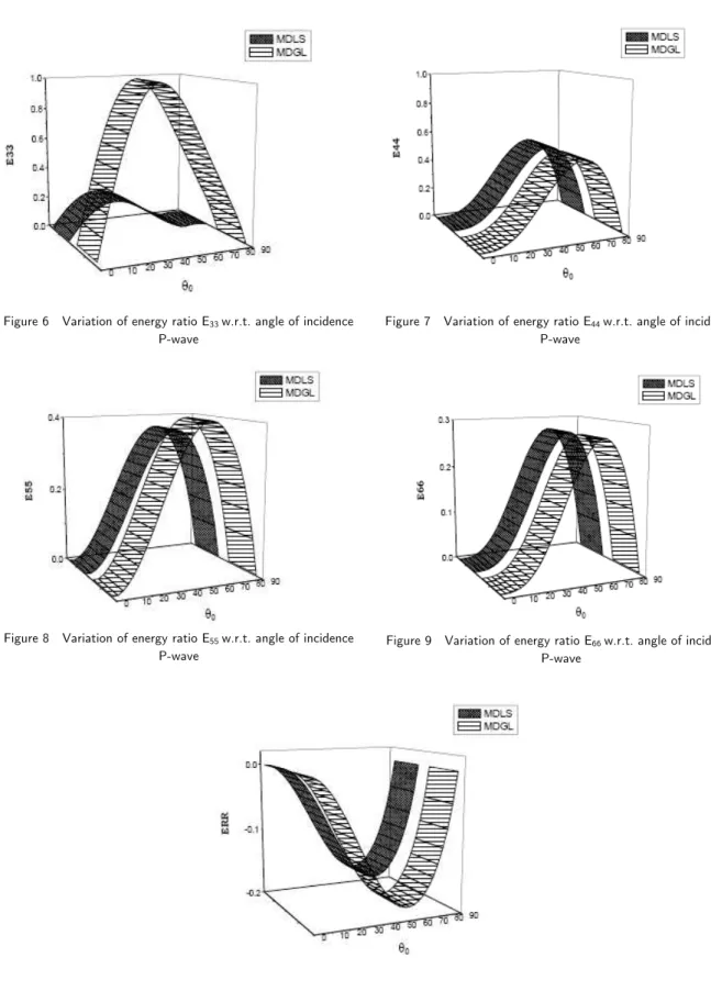
The problem of reflection and refraction phenomenon due to plane waves incident obliquely at a plane interface between uniform elastic solid half-space and microstretch thermoelastic diffusion solid half-space has been studied. It is found that the amplitude ratios of various reflected and refracted waves are functions of angle of incidence, frequency of incident wave and are influenced by the microstretch thermoelastic diffusion properties of the me-dia. The expressions of amplitude ratios and energy ratios are obtained in closed form. The energy ratios have been computed numerically for a particular model. The variations of energy ratios with angle of incidence are shown for thermoelastic diffusion me-dia in the context of Lord-Shulman (L-S) (1967) and Green-Lindsay (G-L) (1972) theories. The conservation of energy at the interface is verified. Some particular cases are also deduced from the present investigation.

Key words

Microstretch, thermoelastic diffusion solid, plane wave, wave propagation, amplitude ratios, energy ratios.

Propagation of plane waves at the interface of an

elastic

solid

half-space

and

a

microstretch

thermoelastic diffusion solid half-space

1 INTRODUCTION

Theory of microstretch continua is a generalization of the theory of micropolar continua.The theory of microstretch elastic solids has been introduced by Eringen [7–10]. This theory is a special case of the micromorphic theory. In the framework of micromorphic theory, a material point is endowed with three deformable directors. When the directors are constrained to have only breathing-type microdeformations, then the body is a microstretch continuum [10]. The material points of these continua can stretch and contract independently of their translations and rotations. A microstretch continuum is a model for a Bravais lattice with its basis on the atomic level and two-phase dipolar solids with a core on the macroscopic level. Composite materials reinforced with chopped elastic fibers, porous media whose pores are filled with gas or inviscid liquid, asphalt, or other elastic inclu-sions and solid–liquid crystals, etc., are examples of microstretch solids. The theory is expected to

Raj n ee s h Kum ar*, a, S. K.G a rgb, Sa nj e ev A h u jac

a_{Department of Mathematics, Kurukshetra} University, Kurukshetra, Haryana, India b_{Department of Mathematics, Deen Bandhu} Chotu Ram Uni. of Sc. & Tech., Sonipat, Haryana,India

c_{University Institute of Engg. & Tech.,} Ku-rukshetra University, KuKu-rukshetra, Haryana, India Received 02 Sep 2012

In revised form 16 Jan 2013 ∗

(2)

Latin American Journal of Solids and Structures 10(2013) 1081 – 1108

find applications in the treatment of the mechanics of composite materials reinforced with chopped fibers and various porous materials.

Eringen [9] developed the theory of microstretch thermoelastic solids and derived the equations of motions, constitutive equations, and boundary conditions for thermo-microstretch fluids and ob-tained the solution of the problem for acoustical waves in bubbly liquids. During the last four dec-ades, wide spread attention has been given to thermoelasticity theories which admit a finite speed for the propagation of a thermal field. Lord and Shulman [18] reported a new theory based on a modified Fourier’s Law of heat conduction with one relaxation time. A more rigorous theory of thermoelasticity by introducing two relaxation times has been formulated by Green and Lindsay (G-L) [13]. A survey article of various representative theories in the range of generalized thermoe-lasticity have been brought out by Hetnarski and Ignaczak [14].

Diffusion is defined as the spontaneous movement of the particles from a high concentration re-gion to the low concentration rere-gion and it occurs in response to a concentration gradient expressed as the change in the concentration due to change in position. Thermal diffusion utilizes the transfer of heat across a thin liquid or gas to accomplish isotope separation. Today, thermal diffusion re-mains a practical process to separate isotopes of noble gases(e.g. xexon) and other light isotopes(e.g. carbon) for research purposes. In most of the applications, the concentration is calculated using what is known as Fick’s law. This is a simple law which does not take into consideration the mutual interaction between the introduced substance and the medium into which it is introduced or the effect of temperature on this interaction. However, there is a certain degree of coupling with tem-perature and temtem-perature gradients as temtem-perature speeds up the diffusion process. The thermod-iffusion in elastic solids is due to coupling of fields of temperature, mass dthermod-iffusion and that of strain in addition to heat and mass exchange with the environment.

Nowacki[19-22] developed the theory of thermoelastic diffusion by using coupled thermoelastic model. Dudziak and Kowalski [6] and Olesiak and Pyryev [23], respectively, discussed the theory of thermodiffusion and coupled quasi-stationary problems of thermal diffusion for an elastic layer. They studied the influence of cross effects arising from the coupling of the fields of temperature, mass diffusion and strain due to which the thermal excitation results in additional mass concentra-tion and that generates addiconcentra-tional fields of temperature. Gawinecki and Szymaniec [11] proved a theorem about global existence of the solution for a nonlinear parabolic thermoelastic diffusion problem. Gawinecki et al. [12] proved a theorem about existence, uniqueness and regularity of the solution for the same problem. Uniqueness and reciprocity theorems for the equations of generalized thermoelastic diffusion problem, in isotropic media, was proved by Sherief et al. [24] on the basis of the variational principle equations, under restrictive assumptions on the elastic coefficients. Due to the inherit complexity of the derivation of the variational principle equations, Aouadi [2] proved this theorem in the Laplace transform domain, under the assumption that the functions of the prob-lem are continuous and the inverse Laplace transform of each is also unique. Sherief and Saleh [25] investigated the problem of a thermoelastic half-space in the context of the theory of generalized thermoelastic diffusion with one relaxation time. Kumar and Kansal [16] developed the basic equa-tion of anisotropic thermoelastic diffusion based upon Green-Lindsay model.

(3)

transmis-Latin American Journal of Solids and Structures 10(2013) 1081 – 1108

sion of the energy of harmonic elastic waves in a bent bar. Sinha and Elsibai [27] discussed the re-flection and refraction of thermoelastic waves at an interface of two semi-infinite media with two relaxation times. Singh [26] studied the reflection and refraction of plane waves at a liquid/thermo-microstretch elastic solid interface. Kumar and Pratap [15] discussed the reﬂection of plane waves in a heat ﬂux dependent microstretch thermoelastic solid half space.

In the present paper, the reflection and refraction phenomenon at a plane interface between an elastic solid medium and a microstretch thermoelastic diffusion solid medium has been analyzed. In microstretch thermoelastic diffusion solid medium, potential functions are introduced to the equa-tions. The amplitude ratios of various reflected and transmitted waves to that of incident wave are derived. These amplitude ratios are further used to find the expressions of energy ratios of various reflected and refracted waves to that of incident wave. The graphical representation is given for these energy ratios for different direction of propagation. The law of conservation of energy at the interface is verified.

2 BASIC EQUATIONS

Following Sherief et al. [24], Eringen [10] and Kumar & Kansal [17].The equations of motion and the constitutive relations in a homogeneous isotropic microstretch thermoelastic diffusion solid in the absence of body forces, body couples, stretch force, and heat sources are given by

λ

₊2

µ

₊_K

(

)

∇ ∇

(

.u

)

−

(

_µ

₊_K

)

∇ × ∇ ×u₊K∇ ×

_ϕ

−

_β

1 1+

τ

1 ∂ ∂t

⎛ ⎝⎜

⎞ ⎠⎟∇T

−β2 1+

τ

1 ∂

∂t

⎛ ⎝⎜

⎞

⎠⎟∇C+

λ

O∇

ϕ

*

=

ρ

∂ 2_u ∂t2 ,

(1)

α

+

β

+

γ

(

)

∇ ∇

(

.

ϕ



)

−

_γ

∇ × ∇ ×

(

_ϕ



)

₊_K∇ ×_u−2K

ϕ

 =

ρ

j∂ 2

ϕ

∂_t2 , (2)

α

0∇ 2

ϕ

*

+

ν

1 T+

τ

1



T

(

)

+

ν

2 C+

τ

1_

C

(

)

−

_λ

1

ϕ

*

−

_λ

0∇.



u=

ρ

j0

2

∂2

ϕ

*

∂_t2 (3)

K

*

∇

2

T

₌

_ρ

C

*

₁

₊

_τ

0

∂

t

⎛

⎝⎜

⎞

⎠⎟



T

₊

_β

1

T

0

1 +

ετ

0

∂

t

⎛

⎝⎜

⎞

⎠⎟

∇

.





u

₊

_ν

1

T

0

1 +

ετ

0

∂

t

⎛

⎝⎜

⎞

⎠⎟

ϕ



*

+

aT

0



C

₊

_γ

1



C

(

)

,

(4)

D

_β

2

ε

kk,ii

+

Dv

2

ϕ

*

,ii

+

Da T

+

τ

1



T

(

)

_,ii

+



C

+

ετ

0

_C

_

(

)

−

Db C

+

τ

1

_C

_

(

)

_,ii

=

0,

(5)

and constitutive relations are

t

_ij

=

λ

u

_r_,_r

δ

_ij

+

µ

(

u

_i_,_j

+

u

_j_,_i

)

+

K u

_j_,_i

−

_ε

ijr

ϕ

r

(

)

−

_β

1

(1

+

τ

1

∂

_t

)

T

δ

ij

−

β

2

(1

+

τ

1

∂

_t

)

C

δ

ij

+

λ

o

δ

ij

ϕ

*

(4)

m

_ij

₌

αϕ

_r_,_r

δ

_ij

+

βϕ

_i_,_j

+

γϕ

_j_,_i

+

b

₀

ε

_mji

ϕ

_,*_m

,

₍₇₎

λ

_i*

=

α

₀

ϕ

_,*_i

+

b

₀

ε

_ijm

ϕ

_j_,_m

,

(8)

where

λ

_,

_µ

_,

_α

_,

_β

_,

_γ

_,

K

_,

_λ

o

,

λ

1

,

α

o

,

b

o

,

are material constants,

ρ

is the mass density ,



u

₌

u

1

,

u

2

,

u

3

(

)

is

the displacement vector and

ϕ



=

(

ϕ

₁

,

ϕ

₂

,

ϕ

₃

)

is the microrotation vector,

ϕ

* is the microstretch scalar function, T and

T

0 are the small temperature increment and the reference temperature of

the body chosen such that

_{T T}

₀

_

1,

C is the concentration of the diffusion material in the elastic body.

K

* is the coefficient of the thermal conductivity,

C

*_{the specific heat at constant}

strain, D is the thermoelastic diffusion constant. a, b are, respectively, coefficients describing the measure of thermodiffusion and of mass diffusion effects,

β

₁

=

(

3λ

+

2 µ

+

K

)

_α

t1

,

β

₂

=

(

3 λ

+

2 µ

+

K

)

_α

c1

,

ν

1

=

(

3 λ

+

2 µ

+

K

)

α

t2

,

ν

2

=

(

3 λ

+

2 µ

+

K

)

α

c2,

α

t1

,

α

t2

are coefficients of linear thermal expansion and

α

c1

,

α

c2 are the coefficients of linear diffusion

expansion.

j

is the microintertia,

j

_o is the microinertia of the microelements,

σ

ij and

m

ij are

components of stress and couple stress tensors respectively,

λ

i

*_{is the microstress tensor,}

e

_ij

₌

1

2 (

u

i,j

+

u

j,i

)

⎛

⎝⎜

⎞

⎠⎟

are components of infinitesimal strain,

e

kk is the dilatation,

δ

_ij is the

Kronecker delta,

τ

0

,

τ

1_{are diffusion relaxation times with}

τ

1

_≥

τ

0

_≥

0

_and

τ

0

,

τ

1 are thermal

relaxation times with

τ

1

≥

τ

0

≥

0

. Here

τ

0

=

τ

0

=

τ

1

=

τ

1

=

γ

1

=

0

for Coupled Thermoelasitc

(CT) model,

τ

1

=

τ

1

=

0,

ε

=

1,

γ

₁

=

τ

₀ for Lord-Shulman (L-S) model and

ε

₌

_0,

_γ

1

=

τ

0

where

τ

0

_>

0

_{for Green-Lindsay (G-L) model.}

In the above equations, a comma followed by a suffix denotes spatial derivative and a super-posed dot denotes the derivative with respect to time respectively.

The basic equations in a homogeneous isotropic elastic solid are written as

λ

e

+

µ

e

(

)

∇

.

∇

u



e

₊

_µ

e

∇

2



u

e

₌

_ρ

e

∂

2



u

e

∂t

2 (9)

where

λ

e

,

µ

e are Lame’s constants,

u

i e

are the components of the displacement vector

u



e,

_ρ

e

is density corresponding to the isotropic elastic solid.

The stress- strain relation in isotropic elastic medium are given by

,

2 =

e _ije e _kke _ij e

ij

e

(5)

where

e

_ije

=

1

2 u

i,j

e

+

u

e_j,i

(

)

⎛

⎝⎜

⎞

⎠⎟

are components of the strain tensor,

e

kk e

is the dilatation.

3 FO R M U LA T IO N O F T H E PR O B LEM

We consider an isotropic elastic solid half-space (M1) lying over a homogeneous isotropic,

mi-crostretch generalized thermoelastic diffusion solid half-space (M2). The origin of the cartesian

coordinate system

(

x

1

,

x

2

,

x

3

)

is taken at any point on the plane surface (interface) and

x

3-axis

point vertically downwards into the microstretch thermoelastic diffusion solid half-space. The elastic solid half-space (M1) occupies the region

x

3

<

0

and the region

x

3

>

0

is occupied by the

microstretch themoelastic diffusion solid half-space (M2) as shown in Fig.1. We consider plane

waves in the

x

1

−

x

3 plane with wave front parallel to the

x

₂-axis. For two-dimensional problem,

we have



u

₌

₍

u

1

,0,

u

3

)

,



ϕ

=

(0,

ϕ

₂

,0)

,

u



e

₌

₍

u

1

e

,0,

u

3 e

)

(11)

(6)

We define the following dimensionless quantities

x₁',x₃'

(

)

=

ω

*

c₁

(

x1,x3

)

, u1 '

,u₃'

(

)

=

ρ

c1

ω

*

β

₁T_o

(

u1,u3

)

,tij '

= tij

β

₁T_o,

t_ije' = tij

e

β

₁T_o,T '

= T

T_o,t '

=

ω

* t,

τ

_o'

=

ω

*

τ

_o,

τ

0'

=

ω

*

τ

0

u

1 e'

,

u

3 e'

(

)

=

ρ

c

1

ω

*

β

₁

T

o

u

1 e

,

u

3 e

(

)

,τ

₁'

=

ω

*

τ

₁

,τ

1'

=

ω

*

τ

1

,

ϕ

*'

=

ρ

c

1 2

β

₁

T

o

ϕ

*

,

λ

i

*'

=

λ

i

*

ω

*

c

1

β

1

T

o

,

ϕ

₂'

=

ρ

c

1 2

β

₁

T

o

ϕ

₂

,

C

'

₌

β

2

C

ρ

2

_c

1 2

m

_ij'

=

ω

*

c

₁

β

₁

T

_o

m

ij

,

(12)

where

ω

*

=

ρ

C

*

c

1 2

K

*

,

c

1 2

=

λ

+

2 µ

+

K

ρ

,

ω

*_{is the characteristic frequency of the medium,}

Upon introducing the quantities (12) in equations (1)-(5), with the aid of (11) and after sup-pressing the primes, we obtain

δ

2

∂e

∂x

1

+

1 −

_δ

2

(

)

∇

2

u

1

−

ζ

1

*

∂

ϕ

2

∂x

3

−

_τ

t 1

∂T

∂x

1

−

_ζ

2 *

τ

c 1

∂C

∂x

1

+

ζ

3 *

∂

ϕ

*

∂x

1

=

∂

2

u

1

∂t

2 (13)

δ

2

∂

e

∂

x

3

+

1 −

_δ

2

(

)

∇

2

u

3

+

ζ

1 *

∂

ϕ

2

∂

x

1

−

_τ

t

1

∂

T

∂

x

3

−

_ζ

2 *

τ

c

1

∂

C

∂

x

3

+

ζ

3

*

∂

ϕ

*

∂

x

3

=

∂

2

u

3

∂

t

2 (14)

ζ

1

∇

2

ϕ

2

+

ζ

2

∂

u

1

∂

x

3

−

∂

u

3

∂

x

1

⎛

⎝⎜

⎞

⎠⎟

−

ζ

3

ϕ

2

=

∂

2

ϕ

2

∂

t

2 (15)

∇

2

T

₌

_τ

t

0

∂

T

∂

t

+



1 *

τ

_e0

∂

e

∂

t

+



2 *

τ

_e0

∂

ϕ

*

∂

t

+



3 *

τ

_c0

∂

C

∂

t

(16)

q

1 *

∇

2

e

+

q

4 *

∇

2

ϕ

*

+

q

2 *

τ

_t1

∇

2

T

+

τ

0_f

∂C

∂t

−

q

3 *

τ

_c1

∇

2

C

=

0

(17)

δ

1 2

∇

2

−

_χ

1 *

(

)

ϕ

*

−

_χ

2 *

e

₊

_χ

3 *

τ

t

1

T

₊

_χ

4 *

τ

c

1

C

₌

∂

2

ϕ

*

(7)

where

ζ

₁

=

γ

j

ρ

c

₁2

,

ζ

2

=

K

j

ρω

*2

,

ζ

3

=

2 K

j

ρω

*2

,

ζ

1

*

=

K

ρ

c

₁2

,

ζ

2

*

=

ρ

c

1

2

β

₁

T

₀

,

ζ

3

*

=

λ

0

ρ

c

₁2

,

δ

2

=

λ

+

µ

ρ

c

₁2



1 *

=

T

0

β

1 2

ρ

K

*

_ω

*

,



2 *

=

β

1

T

0

ν

1

ρ

K

*

_ω

*

,



3 *

=

ρ

c

1 4

a

β

₂

K

*

_ω

*,

q

₁*

₌

D

ω

*

β

₁2

ρ

c

₁4

,

q

2

*

=

D

ω

*

β

₂

a

β

₁

c

₁2

,

q

3

*

=

Db

ω

*

c

₁2

,

q

4

*

=

D

ν

2

β

2

ω

*

ρ

c

₁4

χ

₁*

=

2 λ

ρ

j

₀

ω

*2

,

χ

2 *

=

2 λ

0

ρ

j

₀

ω

*2

,

χ

3 *

=

2 ν

1

c

1

2

j

₀

β

₁

ω

*2

,

χ

4 *

=

2 ν

2

ρ

c

1

4

j

₀

β

₁

β

₂

T

₀

ω

*2

,

δ

1 2

=

c

2

c

₁2 ,

c

2 2

=

2 α

0

ρ

j

₀

,

τ

t 1

=

1 ₊

τ

1

∂

_t

,

τ

c 1

=

1 ₊

τ

1

∂

_t

,

τ

f

0

=

1 ₊

ετ

0

∂

_t

,

τ

t

0

=

1 ₊

τ

0

∂

_t

,

τ

e

0

=

1 ₊

ετ

₀

∂

t

,

τ

c

0

=

1 ₊

γ

₁

∂

t

,

e

₌

∂

u

1

∂

x

1

+

∂

u

3

∂

x

3

,

∇

2

=

∂

2

∂

x

1 2

+

∂

2

∂

x

3 2

We introduce the potential functions

φ

and

_ψ

_{through the relations}

u

1

=

∂

_φ

∂

x

1

−

∂

ψ

∂

x

3

,

u

3

=

∂

_φ

∂

x

3

+

∂

ψ

∂

x

1

,

₍₁₉₎

in the equations (13)-(18), we obtain

∇

2

_φ

−

_τ

t

1

_T

₋

ζ

₂*

τ

c

1

_C

+

ζ

₃*

ϕ

*

=

φ



,

(20)

1 −

_δ

2

(

)

∇

2

ψ

+

ζ

₁*

ϕ

₂

=

_ψ



_,

₍₂₁₎

ζ

₁

∇

2

₋

ζ

₃

(

)

ϕ

₂

−

_ζ

2

∇

2

ψ

=

_ϕ



2

,

(22)

∇

2

T

₌

_τ

t 0

_T



+

τ

e 0



1 *

_∇

2

_φ



+



2 *

_

ϕ

*

(

)

+



3 *

τ

c 0

_C



_,

(23)

q

1 *

∇

4

φ

+

q

4

*

∇

2

ϕ

*

+

q

2

*

τ

_t1

∇

2

T

−

q

3

*

τ

_c1

∇

2

C

+

τ

0_f

_

C

=

0

₍₂₄₎

δ

₁2

_∇

2

₋

χ

₁*

(

)

ϕ

*

₋

χ

₂*

_∇

2

φ

+

χ

₃*

τ

t 1

_T

+

χ

₄*

τ

c

1

_C

=

_ϕ



*

,

₍₂₅₎

For the propagation of harmonic waves in

x

(8)

φ

,ψ

,

T

_,

C

_,ϕ

*

_,ϕ

2

{

}

(

x

1

,

x

3

,

t

)

=

φ

,ψ

,

T

,

C

,ϕ

*

,ϕ

₂

{

}

e

−iωt ₍₂₆₎

where

ω

_{is the angular frequency}

Substituting the values of

φ

,ψ

,

T

,

C

_,ϕ

*

_,ϕ

2 from equation (26) in the equations (20)-(25), we

obtain

∇

2

₊

_ω

2

(

)

ϕ

−

_τ

t

''

_T

+

ζ

3

*

ϕ

*

₋

ζ

₂*

τ

c

''

_C

=

0,

₍₂₇₎

1 −

_δ

2

(

)

∇

2

₊

_ω

2

(

)

ψ

+

ζ

₁*

ϕ

₂

=

0,

₍₂₈₎

ζ

₂

∇

2

ψ

+

−

_ω

2

₋

ζ

₁

∇

2

+

ζ

₃

(

)

ϕ

₂

=

0,

₍₂₉₎



1 *

τ

e

10

_∇

2

ϕ

+

τ

t

10

_{− ∇}

2

(

)

T

₊



2 *

τ

e

10

ϕ

*

+



3 *

τ

c

10

_C

=

0,

₍₃₀₎

q

₁*

∇

4

ϕ

+

q

₄*

∇

2

ϕ

*

+

q

₂*

τ

_t''

∇

2

T

+

τ

10_f

−

q

₃*

τ

_c''

∇

2

(

)

C

=

0;

₍₃₁₎

−

_χ

2

*

_∇

2

ϕ

+

χ

₃*

τ

t

''

_T

+

r

1

ϕ

*

+

r

2

C

=

0,

(32)

where

r

₁

₌

δ

₁2

_∇

2

₋

χ

₁*

+

ω

2

,r

₂

₌

χ

₄*

(1

−

_i

_ω

_),

_τ

t 11

=

(1

−

_i

_ωτ

1

),

τ

c

11

=

(1

−

_i

_ωτ

1

),

τ

_e10

=

−

_i

_ω

₍₁

−

_i

_ωετ

0

),

τ

t

10

=

−

_i

_ω

₍₁

−

_i

_ωτ

0

),

τ

c

10

=

−

_i

_ω

₍₁

−

_i

_ωγ

_),

_τ

f 10

=

−

_i

_ω

₍₁

−

_i

_ωετ

0

₎

The system of equations (27), (30)-(32) has a non-trivial solution if the determinant of the co-efficients

⎡

_⎣

ϕ

,

T

_,

_ϕ

*

_,

C

⎤

_⎦

T

vanishes, which yields to the following polynomial characteristic equation

∇

8

+

B

1

∇

6

+

B

2

∇

4

+

B

3

∇

2

+

B

4

=

0

(33)

where

B

_i

₌

A

_i

A for

(

i

₌

1,2,3,4),

A

₌

g

₁*

₋

a

₁₄

g

₁₄*

,

A

₁

₌

g

*₂

₊

g

₁*

ω

2

₋

_a

12

g

6

*

+

a

₁₃

g

₉*

₋

a

₁₄

g

₁₂*

,

A

₂

₌

g

₃*

₊

g

₂*

ω

2

₋

_a

12

g

7 *

+

a

₁₃

g

₁₀*

₋

a

₁₄

g

₁₃*

,

A

₃

₌

g

₄*

₊

g

₃*

ω

2

₋

_a

12

g

8

*

+

a

₁₃

g

₁₁*

,

A

₄

₌

g

₄*

ω

2

_,

(9)

g

₁*

=

−

δ

1

2

a

₄₆

,

g

₂*

=

a

₂₃

a

₄₆

−

_a

24

a

43

+

δ

1 2

(

a

₃₂

a

₄₆

+

a

₄₅

+

a

₃₄

a

₄₂

),

g

₄*

=

a

₄₅

(

a

₂₂

a

₃₃

+

a

₂₃

a

₃₂

),

g

₃*

=

−

_a

33

(

a

22

a

46

+

a

24

a

42

)

−

a

23

(

a

32

a

46

+

a

45

+

a

34

a

42

)

+

a

43

(

a

24

a

32

−

a

22

a

34

)

−

δ

1 2

a

₃₂

a

₄₅

,

g

₆*

=

δ

1

2

(

a

₃₁

a

₄₆

+

a

₄₁

a

₃₄

),

g

₇*

₌

a

₃₃

(

−

_a

21

a

46

−

a

24

a

41

)

−

a

23

(

a

31

a

46

+

a

34

a

41

)

+

(

a

24

a

31

−

a

21

a

34

)

a

43

−

δ

1 2

a

₃₁

a

₄₅

,

g

₈*

=

a

₄₅

(

a

₂₃

a

₃₁

+

a

₂₁

a

₃₃

),

g

₉*

=

a

₂₄

a

₄₁

+

a

₂₁

a

₄₆

,

g

₁₀*

=

−

_a

21

(

a

32

a

46

+

a

45

+

a

34

a

42

)

+

a

22

(

a

31

a

46

+

a

34

a

41

)

+

a

24

(

a

31

a

42

−

a

32

a

41

)

g

₁₁*

=

a

₄₅

(

a

₂₁

a

₃₂

−

a

₂₂

a

₃₁

),

g

₁₂*

=

−(

a

₂₃

a

₄₁

₊

a

₂₁

a

₄₃

)

₊

δ

₁2

(

a

₃₁

a

₄₂

−

a

₄₁

a

₃₂

),

a

₄₅

₌

τ

10_f

,

a

₄₆

₌

q

₃*

τ

_c11

g

₁₃*

=

a

₃₃

(

a

₂₂

a

₄₁

−

a

₂₁

a

₄₂

)

+

a

₂₃

(

a

₃₂

a

₄₁

−

a

₃₁

a

₄₂

)

+

a

₄₃

(

a

₂₁

a

₃₂

−

a

₂₂

a

₃₁

),

g

₁₄*

=

δ

₁2

a

₄₁

,

a

₁₁

=

∇

2

+

ω

2

,

a

₂₁

=

−

χ

₂*

,

a

₃₁

=



1 *

τ

_e10

,

a

₄₁

=

q

₁*

,

a

₁₂

=

−

τ

_t11

,

a

₂₂

=

χ

₃*

τ

_t11

,

a

₃₂

=

τ

_t10

,

a

₄₂

=

q

₂*

τ

_t11

,

a

₁₃

=

ζ

₃*

,

a

₂₃

=

χ

₁*

−

ω

2

,

a

₄₃

=

q

₄*

∇

2

,

a

₃₃

₌



2 *

τ

_e10

,

a

₁₄

₌

−

ζ

₂*

τ

_c11

,

a

₂₄

₌

r

₂

,

a

₃₄

₌



3 *

τ

_c10

,

a

₄₄

₌

(

a

₄₅

−

a

₄₆

∇

2

),

The general solution of equation (33) can be written as

ϕ

₌

ϕ

_i

i₌₁ 4

∑

(34)

where the potentials

ϕ

i

,

i

=

1,2,3,4

are solutions of wave equations, given by

∇

2

+

ω

2

V

i 2

⎡

⎣

⎢

⎤

⎦

⎥

ϕ

i

=

0,

i

=

1,2,3,4

(35)

Here

V

i

2

,

i

₌

_1,2,3,4

(

)

are the velocities of four longitudinal waves, that is, longitudinal dis-placement wave (LD), mass diffusion wave (MD), thermal wave (T) and longitudinal mi-crostretch wave (LM) and derived from the roots of the biquadratic equation in

V

2_{, given by}

B

4

V

8

−

B

3

ω

2

V

6

₊

B

2

ω

4

V

4

₋

B

1

ω

6

V

2

₊

ω

8

(

)

=

0

₍₃₆₎

(10)

(

ϕ

,

T

_,

_ϕ

*

_,

C

₎

₌

_(1,

k

1i

,

k

2i

,

k

3i

)

ϕ

i

1 4

∑

(37)

where

* 6 * 4 2 * 2 4 * 6 * 4 2 * 2 4

1 6 7 8 2 9 10 11

* 8 * 6 2 * 4 4 2 * 6 * 4 2 * 2 4 * 6

3 14 12 13 1 2 3 4

(

)

,

(

)

,

(

) (

),

(

),

1, 2,3, 4

d d

i i i i i i

d d

i i i i i i i

k

g

V

g

V

k

g

V

g

V

k

g

V

g

V

V k

k

g

V

g

V

g V

i

ω

=

−

₊

₌

−

₊

=

−

₊

−

₌

₊

₌

The system of equations (28)-(29) has a non-trivial solution if the determinant of the coeffi-cients

⎡⎣

ψ

,

ϕ

₂

⎤⎦

T vanishes, which yields to the following polynomial characteristic equation

∇

4

₊

_A

*

∇

2

₊

_B

*

₌

0

₍₃₈₎

where

A

*

=

ω

2

ζ

₁

+

ζ

₁*

ζ

₂

−

1 ₋

δ

2

(

)

ζ

₃

+

ω

2

(

)

(

)

1 ₋

δ

2

(

)

ζ

₁

,

_B

*

₌

ω

2

ω

2

−

ζ

₃

(

)

1 ₋

δ

2

(

)

ζ

₁

The general solution of equation (38) can be written as

ψ

=

ψ

i

i₌5 6

∑

(39)

where the potentials

ψ

i

,

i

=

1,2

are solutions of wave equations, given by

∇

2

+

ω

2

V

i 2

⎡

⎣

⎢

⎤

⎦

⎥

ψ

i

=

0,

i

=

5,6

(40)

Here

V

i

2

,

i

₌

_5,6

(

)

are the velocities of two coupled transverse displacement and microrota-tional (CD I, CD II) waves and derived from the root of quadratic equation in

V

2_{, given by}

B

*

V

4

₋

A

*

ω

2

V

2

₊

ω

4

(

)

=

0

₍₄₁₎

Making use of equation (39) in the equations (28)-(29) with the aid of equations (26) and (40), the general solutions for

ψ

and

_ϕ

2 are obtained as

ψ

,

ϕ

₂

{

}

=

1,

n

1i

{

}

ψ

i i₌5

6

(11)

where

n

_1i

₌

ζ

2

ω

2

ζ

₃

−

ω

2

(

)

V

_i2

₊

ζ

₁

ω

2

for i

=

5,6

Applying the dimensionless quantities (12) in the equation (9) with the aid of (11) and after suppressing the primes, we obtain

α

e2

−

β

e2

c

1 2

⎛

⎝

⎜

⎞

⎠

⎟

∂

e

∂

x

1

⎛

⎝⎜

⎞

⎠⎟

+

β

e2

c

1

2

∇

2

_u

1

e

=

u



1

e

(43)

α

e2

−

β

e2

c

1 2

⎛

⎝

⎜

⎞

⎠

⎟

∂

e

∂

x

3

⎛

⎝⎜

⎞

⎠⎟

+

β

e2

c

1 2

∇

2

u

3 e

=

u



3 e

(44)

where

e

₌

∂

u

1 e

∂

x

1

+

∂

u

3 e

∂

x

3

⎛

⎝⎜

⎞

⎠⎟

and

α

e

=

λ

e

+

2µ

e

(

)

ρ

e

,

β

e

=

µ

e

ρ

e

are velocities of longitudinal wave (P-wave) and trans-verse wave (SV-wave) corresponding to M1, respectively.

The components of

u

1

e

and

u

3 e

are related by the potential functions as:

u

1

e

=

∂

ϕ

e

∂

x

1

-

∂

ψ

e

∂

x

3

,

u

3

e

=

∂

ϕ

e

∂

x

3

+

∂

ψ

e

∂

x

1

, ₍₄₅₎

where

ϕ

e

and

ψ

e

satisfy the wave equations as

∇

2

_ϕ

e

=

ϕ



e

α

2 ,

∇

2

_ψ

e

=

ψ



e

β

2 , (46)

and

α

₌

α

e

c

1,

β

=

β

e

c

1.

4 REFLECTION AND REFRACTION

We consider a plane harmonic wave (P or SV) propagating through the isotropic elastic solid half-space and is incident at the interface

x

3

=

0

as shown in Fig.1. Corresponding to each

(12)

inhomogeneous waves (LD, MD, T, LM, CD I and CD II) are transmitted in isotropic mi-crostretch thermoelastic diffusion solid half-space.

In elastic solid half-space, the potential functions satisfying equation (46) can be written as

φ

e

=

A

0 e

e

{

iω(x1sinθ0+x3cosθ0)/α−t

}

+

A

1 e

e

{

iω(x1sinθ1+x3cosθ1)/α−t

}

(47)

ψ

e

=

B

0 e

e

{

iω(x1sinθ0+x3cosθ0)/β−t

}

+

B

1 e

e

{

iω(x1sinθ2+x3cosθ2)/β−t

}

(48)

The coefficients

A

0

e

(

B

0

e

),

A

1 e

and

B

1

e

are amplitudes of the incident P (or SV), reflected P and reflected SV waves respectively.

Following Borcherdt [3], in a homogeneous isotropic microstretch thermoelastic diffusion half-space, potential functions satisfying equations (35) and (40) can be written as

ϕ

,

T

_,

_ϕ

*

,

C

(

)

=

1,

k

1i

,

k

2i

,

k

3i

{

}

i₌1 4

∑

B

i

e

(

 Ai.r)

_e

i(

 Pi.r−ωt)

{ }

(49)

(

)

{ }

6

( . ) ( . )

2 5

,

{1,

}

A ri i P ri t

ip i i

n B e

e

ω

ψ φ

−

=

∑

v r r r

(50)

The coefficients

B

i,

i

=

1,2,3,4,5,6

are the amplitudes of refracted waves. The propagation

vector

P



_i_,

i

₌

1,2,3,4,5,6

and attenuation

A



i factor (

i

=

1,2,3,4,5,6

) are given by



P

_i₌

ξ

R

x

ˆ

1

+

dV

i R

x

ˆ

3,



A

_i₌

−ξ

I

x

ˆ

1

−

dV

i I

x

ˆ

3,

i

=

1,2,3,4,5,6

(51)

where

dV

_i

₌

dV

_{i R}

₊

i dV

_{i I} _{= p.v.}

ω

2

V

i 2

−

ξ

2

⎛

⎝

⎜

⎞

_⎠

⎟

1

2

,

i

₌

_1,2,3,4,5,6

(52)

and

ξ

=

ξ

R

+

i

ξ

I is the complex wave number. The subscripts R and I denote the real and imaginary

parts of the corresponding complex number and p.v. stands for the principal value of the complex quantity derived from square root. ξR ≥ 0 ensures propagation in positive

x

₁-direction. The

com-plex wave number ξ in the microstretch thermoelastic diffusion medium is given by

ξ

₌

P



i

sin

θ

i

′

−

i



A

(13)

where

γ

i,

i

=

1,2,3,4,5,6

is the angle between the propagation and attenuation vector and

θ

i

′

,

i

₌

_1,2,3,4,5,6

_{is the angle of refraction in medium II.}

5 B O U N D A R Y C O N D IT IO N S

The boundary conditions are the continuity of stress and displacement components, vanishing of the gradient of temperature, mass concentration, the tangential couple stress and microstress components. Mathematically these can be written as

Continuity of the normal stress component

33

=

33

,

e

t

₍₅₄₎

Continuity of the tangential stress component

t

31

e

=

t

31

,

(56)

Continuity of the tangential displacement component

u

1

e

=

u

1, (57)

Continuity of the normal displacement component

u

3

e

=

u

3, (58)

Vanishing the gradient of temperature

∂

T

∂

x

3

=

0

, ₍₅₉₎

Vanishing the mass concentration

∂C

∂x

3

=

0

, ₍₆₀₎

Vanishing of the tangential couple stress component

m

32

=

0

(61)

(14)

λ

3 *

=

0

₍₆₂₎

Making the use of potentials given by equations (47)-(50), we find that the boundary condi-tions are satisfied if and only if

ξ

_R =

ω

sin

θ

0

V

₀ =

ω

sinθ

₁

α

=

ω

sin

_θ

₂

β

(63)

and

ξ

_I = 0. (64)

where

V

₀₌

α

,

for incident P

−

wawe

β

,

for incident SV

−

wawe

⎧

⎨

⎩

(65)

It means that waves are attenuating only in

x

3-direction. From equation (53), it implies that

if



A

i

≠

0

, then

γ

i

'

=

θ

_i

′

,

i

₌

1,2,3,4,5,6

, that is, attenuated vectors for the six refracted waves are directed along the

x

3-axis.

Using equations (47)-(50) in the boundary conditions (54)-(62) and with the aid of equations (19), (45), (63)-(65), we get a system of eight non-homogeneous equations which can be written as

d

ij j=1

8

∑

Z

j

=

g

i (66)

where

Z

_j

=

Z

_j

e

iψj *

,

Z

_j

,

ψ

*_j

,

j

=

1,2,3,4,5,6,7,8

represents amplitude ratios and phase shift of reflected P-, reflected SV-, refracted LD-, refracted MD-, refracted T-, refracted LM-, refracted CD I -, refracted CD II - waves to that of amplitude of incident wave, respectively.