Lat. Am. j. solids struct. vol.10 número6

(1)

A b stract

Abstract: In this paper, a shell finite element formulation to analyze highly deformable shell structures composed of homogeneous rubber-like materials is presented. The element is a triangular shell of any-order with seven nodal parameters. The shell kinematics is based on geometrically exact Lagrangian description and on the Reissner-Mindlin hypothesis. The finite element can represent thickness stretch and, due to the seventh nodal parameter, linear strain through the thickness direction, which avoids Poisson locking. Other types of lock-ing are eliminated via high-order approximations and mesh refinement. To deal with high-order approximations, a numerical strategy is devel-oped to automatically calculate the shape functions. In the present study, the positional version of the Finite Element Method (FEM) is employed. In this case, nodal positions and unconstrained vectors are the current kinematic variables, instead of displacements and rota-tions. To model near-incompressible materials under finite elastic strains, which is the case of rubber-like materials, three nonlinear and isotropic hyperelastic laws are adopted. In order to validate the pro-posed finite element formulation, some benchmark problems with materials under large deformations have been numerically analyzed, as the Cook’s membrane, the spherical shell and the pinched cylinder. The results show that the mesh refinement increases the accuracy of solutions, high-order Lagrangian interpolation functions mitigate gen-eral locking problems, and the seventh nodal parameter must be used in bending-dominated problems in order to avoid Poisson locking.

Ke ywo rd s

large deformation analysis; homogeneous rubber-like materials; shell finite elements.

A shell finite element formulation to analyze highly

deformable rubber-like materials

1 INTRODUCTION

Highly deformable elastic shell structures have been widely used in engineering, therefore the ade-quate prediction of the behavior of such structures is an essential step during the design process. In this context, the search for a reliable prediction method has been objective of several studies along

J. P . P as con* an d H . B . Co da

Department of Structural Engineering, São Carlos School of Engineering, Uni-versity of São Paulo, São Carlos, São Paulo, Brazil

Received 25 Sep 2012 In revised form 25 Jan 2013

(2)

Latin American Journal of Solids and Structures 10(2013) 1177 – 1209

the last decades. One way to analyze the mechanical behavior of structures is the use of numerical or approximate methods, as the Finite Element Method (FEM). In general, these methods are more practical and more efficient when compared to experimental methods, and analytical solutions are available only for simplified cases. In this paper, an isoparametric triangular shell finite element of any-order is employed to describe large displacements and large strains developed in general rubber-like applications.

In order to reduce the computational effort, some researchers have attempted to improve the accuracy of the results provided by coarse meshes and low-order elements via alternative methods as, for instance, the reduced integration, the selective reduced integration, the enhanced assumed strain (EAS) method, the assumed natural strain (ANS) method and the hourglass stabilization methods. However, as pointed out by [1], these modified low-order elements tend to lack reliability and are case-dependent, which makes them difficult to be implemented in finite element codes. In general, elements of sufficiently high orders are more reliable, robust and their performance is less case-dependent. Despite the computational effort required, the use of fully integrated finite elements of higher orders tends to mitigate most types of locking, increasing the reliability of the formulation (see, for instance, [2], [3], [4] and [5]). High-order shell finite elements are successfully employed, for example, in [5-10].

Regarding the shell kinematics, one may employ the Reissner-Mindlin hypothesis, in which the material fibers initially straight and normal to the undeformed mid-surface remain straight but not necessarily normal to the deformed mid-surface. So, unlike the Kirchhoff-Love theory, the shear strains are taken into account, and the shell kinematics depends on the mid-surface displacements and on the vector that maps the material points out of the mid-surface, called director vector. In this context, there are three classes of shell finite element usually employed in the scientific litera-ture: the 5-parameter shells, in which the director remains unitary and, thus, the thickness does not change with deformation; the 6-parameter shells, in which the director does not remain unitary and, then, the thickness can change with deformation; and the 7-parameter shells, in which thickness change and a linearly variable strain through the thickness direction are considered. For the first class of shells, there are five degrees of freedom per node: three displacements of the shell mid-surface, and two components of the director (the third component can be found by using the hy-pothesis of a unitary deformed director). The 5-parameter shell formulation can be used to describe membrane and shear strains. The sixth parameter introduced is related to the thickness stretch - or the transverse normal strains (see, for example, [11], and [12]). Finally, in order to eliminate the Poisson thickness locking in bending-dominated shells, the seventh parameter has been included. This additional degree of freedom represents the linear variation of the (transverse) strain across the thickness direction and, as pointed out by [13], was firstly proposed by [14]. According to [10], the Poisson thickness locking does not decrease with mesh refinement of a six parameter formulation and, thus, the seventh parameter is necessary.

(3)

coordi-Latin American Journal of Solids and Structures 10(2013) 1177 – 1209

nates. An alternative procedure, which avoids the abovementioned difficulties, is the positional ver-sion of the FEM (see, for instance, [15], [16] and [9]). In this case, the seven nodal degrees of free-dom of the shell are: three components of the current shell reference surface; three components of the final deformed unconstrained director; and the final linear strain rate across the thickness. In [9], the approximation order of the 7-parameter triangular shell finite element used is cubic and a linear Saint Venant-Kirchhoff constitutive relation is employed. In this paper, the element order is generalized, i.e., the approximation degree can be any one (low, moderate or high), and rubber-like constitutive relations are adopted.

Regarding finite elastic deformations, two engineering applications can be cited: metals, which can present large displacements with small strains; and rubber-like materials, which can also pre-sent large strains. In order to describe finite displacements, the geometrically nonlinear analysis together with the Nonlinear Continuum Mechanics is employed in the present study. Further de-tails can be found in [17], [18] and [19], for instance. The modeling of finite strains is performed here by means of nonlinear isotropic hyperelastic laws, often used to describe the response of homogene-ous rubber-like materials (see, for example, [3, 20-24]).

Concerning studies about shell finite elements with linearly variable strain through the thick-ness and composed of homogeneous rubber-like materials, one can cite the following papers: [12], [25], [26] and [27]. In the first two studies, the material incompressibility condition is adopted and the transverse shear strains are neglected. In [26] and [27], finite rotations are treated by the Euler-Rodrigues formula, but in the first of these studies, condensation of the three-dimensional constitu-tive model is performed via a consistent plane stress condition. In this paper, the constituconstitu-tive model is fully three-dimensional, the shear strains are considered and, as mentioned previously, no rotation formulae are employed.

The purpose of the present study is to describe a numerical formulation with isoparametric tri-angular shell finite elements of any-order, accounting for thickness stretch and linear strain varia-tion across the thickness, in order to analyze homogeneous elastic shells under statically applied forces, isothermal conditions, finite displacements and finite strains. One contribution of this paper is to cover the lack in the assessment of the seven-parameter shell performance under large-strain problems. In [6] and [9], for example, high-order hyperelastic shells with linear strain rate across the thickness are employed, but only the Saint Venant-Kirchhoff model is used in the numerical exam-ples. Moreover, the present finite element formulation can be easily implemented in a computer code for any order of approximation.

(4)

2 FIN IT E E LE M E N T M A P P IN G

The finite element adopted in the present study is briefly described in this section. The element is a triangular shell of any-order with seven nodal parameters, similar to the shell element of cubic order used in [9]. For both initial (

x

) and current (

y

) element configurations, the material points can be split into two groups: the reference surface points, and the external points. To nu-merically describe the position of the reference surface points, the following expressions are em-ployed:

x

_i

( )

m

=

X

_iL

φ

_L

(

ξ

₁

,

ξ

₂

)

(1)

y

_i

( )

m

=

Y

_iL

φ

_L

(

ξ

₁

,

ξ

₂

)

(2)

where

X

_iL and

Y

_iL are, respectively, the initial and the current positions of node L;

φ

_L is the shape function associated with node L; and the non-dimensional coordinates

ξ

₁ and

ξ

₂ belong to the triangular auxiliary space defined by the set

{

(

ξ

₁

,

ξ

₂

)

∈



2

/ 0

≤ ξ

₁

,

ξ

₂

,

ξ

₁

₊

ξ

₂

≤

1 }

.

The external points of the shell, which are out of the reference surface, are mapped from a vector defined at the shell mid-surface and represented here by

g

:

x

i

=

( )

x

i m

+

g

0

( )

_i (3)

g

₀

( )

_i

=

h

0

2 n

i

0

_ξ

1

,ξ

2

(

)

⎡

⎣

⎤

⎦ξ

3

=

( )

d

0 _i

ξ

₃

2

(4)

y

_i

=

( )

y

_i m

+

( )

g

₁

i (5)

g

₁

( )

_i

=

h

2 n

i 1

_ξ

1

,ξ

2

(

)

⎡

⎣

⎤

⎦ ξ

3

+

a

(

ξ

1

,ξ

2

)

ξ

3 2

⎡

⎣

⎤

⎦

=

h

₂

0

g

i 1

_ξ

1

,ξ

2

(

)

⎡

⎣

⎤

⎦

ξ

3

+

a

(

ξ

1

,ξ

2

)

ξ

3 2

⎡

⎣

⎤

⎦

=

d

₁

( )

_i

ξ

3

+

a

(

ξ

1

,

ξ

2

)

ξ

3 2

⎡

⎣

⎤

⎦

2

(6)

where the superscript m denotes the reference surface points (equations 1 and 2);

ξ

3 is the third

non-dimensional coordinate (

−

1 _{≤ ξ}

3

≤

1

);

n

denotes a unit vector, whose direction defines the

points that are out of the reference surface;

h

0 and

h

are the initial and the current shell

thick-ness;

d

0 and

d

₁ are the initial and final directors, respectively; and variable

a

is the rate of

(5)

vector

d

_{into its rotational and extensional components (that is, the use of}

d

₌

_h

n

) must be done in order to avoid ill-conditioning in the thin shell limit. The initial unit normal vector

n

0

(equation 4), the vector

g

1 (equation 6) and the rate

a

(equation 6) are also interpolated via

their corresponding nodal values and shape functions:

n

_i0

(

ξ

₁

,

ξ

₂

)

=

( )

N

0_i L

φ

_L

(

ξ

₁

,

ξ

₂

)

(7)

g

1_i

(

ξ

₁

,

ξ

₂

)

₌

G

_iL

φ

_L

(

ξ

₁

,

ξ

₂

)

(8)

a

(

ξ

₁

,

ξ

₂

)

=

A

L

φ

_L

(

ξ

₁

,

ξ

₂

)

₍₉₎

where

N

0_{represents the nodal values of the unit vector}

n

0_;

G

i L

denotes the nodal values of the

vector

g

1_i; and

A

L is the value of variable

a

at node

_L

. The initial unit vector (

_n

0) is normal

to the mid-surface, but the current unit vector (

n

1) is not necessarily normal to the current mid-surface. In general, the vector

g

1 is neither unitary nor normal to the shell mid-surface. Except for linear approximation order, the shell elements can be curved. As in the study of [9], there are seven parameters - or degrees of freedom - per node (L): three current positions of the shell mid-surface (

Y

₁L,

Y

₂L and

Y

3 L

), three components of the vector

g

1 (

G

1 L

,

G

2 L

and

G

3 L

), and the nodal value of variable

a

(

_A

L). To reproduce a simply supported node, for instance, one should restrict the translational degrees of freedom

Y

₁L,

Y

₂L and

Y

3 L

, and to clamp the element edge,

one should also restrict the components of vector

g

1 along the nodes of this edge. Other shell formulations, which can also numerically describe thickness change and linear strain across the thickness direction are presented by [14], [28], [29], [30], [31], [5] and [9], among others.

Regarding Nonlinear Continuum Mechanics strain measures, the following Lagrangian quanti-ties are used in this paper:

F

₌

∂

y

∂

_x

or

F

ij

=

∂

_y

i

∂

_x

j

₍₁₀₎

J

₌

det

( )

_F

₍₁₁₎

C

₌

F

T

F

_or

_C

ij

=

F

ki

F

kj (12)

E

₌

1

2 C

₋

I

(

)

or

E

_ij

=

1

2 C

ij

− δ

ij

(6)

where

F

is the (material) deformation gradient;

J

_{is the Jacobian;}

C

_{is the right Cauchy-Green}

stretch tensor;

E

is the Green-Lagrange strain tensor; and the symbols

I

and

δ

_denote,

respec-tively, the identity matrix and the Kronecker delta.

The numerical determination of the deformation gradient

F

(equation 10) is performed as:

F

=

( )

F

1

( )

F

0 −1

or

F

_ij

=

( )

F

₁

ik

( )

F

0 −1

⎡

⎣⎢

⎤

⎦⎥

_kj (14)

F

0

=

∂

x

∂ξ

or

( )

F

0 _ij

=

∂

x

_i

∂ξ

_j (15)

F

₁

=

∂

y

∂ξ

or

( )

F

1 _ij

=

∂

y

_i

∂ξ

_j (16)

The position vectors

x

and

y

map the material points of the shell element, respectively at the initial and the current configurations, from the non-dimensional space

ξ

=

{

ξ

₁

,

ξ

₂

,

ξ

₃

}

.

3 H Y P ER ELA ST IC C O N ST IT U T IV E LA W S

In this study, the (macroscopic) material behavior is mathematically described by means of hy-perelastic constitutive laws, in which the material response is derived from a scalar potential called Helmholtz free-energy function and represented here by

ψ

. Three nonlinear hyperelastic constitutive laws are employed here: the Hartmann-Neff model, denoted here by HN; and two neo-Hookean models, denoted here by nH1 and nH2. Such models can be used for isotropic and near-incompressible rubber-like materials. The mathematical expressions of these models are [21, 22, 24]:

ψ

HN

=

k

50 J

5

+

J

−5

−

2 ⎡⎣

⎤⎦

+

d i

1 3

−

27 ⎛

⎝

⎠

⎞

+

c

10

(

i

1

−

3

)

+

c

01

i

2 3/2

−

3

3/2

⎛

⎝

⎞

⎠

(17)

ψ

nH1

=

k

2 ln J

( )

⎡

⎣

⎤

⎦

2

+

µ

2 i

1

−

3 −

2 ln J

( )

⎡

⎣

⎤

⎦

(18)

ψ

nH 2

=

k

4 J

2

−

1 −

ln J

( )

2

⎡

⎣

⎤

⎦

+

µ

2 i

1

−

3 ⎡

⎣

⎤

⎦

(19)

(7)

where

k

is the bulk modulus;

d

_,

c

10 and

c

01 are the isochoric coefficients of the HN model [21];

µ

is the shear modulus;

J

_{is the Jacobian (equation 11); and the invariants}

_i

1,

i

2 and

i

1 are

given by (see equation 12):

i

1

=

tr

( )

C

=

tr J

−2/3

C

⎡

⎣

⎦

⎤

=

J

−2/3

tr

( )

C

=

J

−2/3

C

kk (20)

i

2

=

tr

C

−1

⎛

⎝

⎞

⎠

=

tr

J

−

2/3

C

(

)

−1

⎡

⎣⎢

⎤

⎦⎥

=

J

−2/3

C

(

)

−1

⎡

⎣⎢

⎤

⎦⎥

kk (21)

i

1

=

tr

( )

C

=

C

kk (22)

where

tr

( )

_{is the trace operator. For both models, as the Jacobian}

J

_{is a measure of volumetric}

change, one can highlight two aspects: the near-incompressibility condition (

J

_≈

1

_{) can be}

achieved by setting a bulk modulus much larger than the other material coefficients [3, 21, 23]; and the energy

ψ

tends to infinity as

J

_{tends to zero, which represents the impossibility of}

an-nihilating the material (

J

₌

0

_{). Besides, the normalization condition is satisfied, that is, the}

ener-gy

ψ

is zero if the material is under a rigid-body motion (

C

₌

I

_).

In hyperelasticity, the relation among the Helmholtz free-energy function

ψ

, the Green-Lagrange strain tensor

E

(equation 13) and the stress tensor, used to describe the material be-havior, is:

S

₌

∂ψ

∂

E

=

2 ∂ψ

∂

C

or

S

ij

=

∂ψ

∂E

_ij

=

2 ∂ψ

∂C

_ij (23)

where

S

_{is the symmetric second Piola-Kirchhoff stress tensor. The derivatives of the Helmholtz}

free-energy function (

ψ

) in respect to the right Cauchy-Green stretch tensor (

C

_{), for the}

hyper-elastic models (17), (18) and (19), can be found, for instance, in [19] and [23].

4 EQ U ILIB R IU M

In the present study, the equilibrium of each shell element and hence of the whole structure is described by the Minimal Total Potential Energy Principle, also called Principle of Stationary Total Potential Energy. The static equilibrium of forces is achieved if the following condition is satisfied:

f

int

=

f

int

( )

y

=

∂ψ

∂

y

Ω0

∫

dV

0

=

f

ext or

( )

F

int _i

=

∂ψ

∂

y

_i Ω

∫

₀

dV

₀

₌

( )

F

_ext

(8)

where

f

int is the internal force vector, which depends on the current configuration

y

(see section

2);

Ω

0 and

dV

0 denote, respectively, the initial domain and an infinitesimal volume element at the initial position; and

f

ext is the vector of external (applied) forces. Similarly to [9], as the

equi-librium condition (24) gives rise to a nonlinear system of equations, the Newton-Raphson iterative technique is employed to achieve the solution. In order to apply this technique, the following equations are used:

r

=

f

int

( )

y

−

f

ext or

r

i

=

( )

f

int _i

−

( )

f

ext _i (25)

H

=

∂

r

∂

y

=

∂

f

_int

∂

y

−

∂

f

_ext

∂

y

=

∂

2

ψ

∂

y

∂

y

Ω0

∫

dV

0 or

H

ij

=

∂

2

_ψ

∂

y

_i

∂

y

_j Ω

∫

₀

dV

0 (26)

y

₌

y

₊

Δ

y

₌

y

−

H

−1

⋅

r

or

y

_i

=

y

_i

−

( )

H

−1

ij

r

j (27)

where

r

is the residual force vector, also called out-of-balance force vector; and

H

is the Hessian matrix. The current position (

y

) is update via equation (27) until the following norm is smaller than a given tolerance:

norm

₌

norm

1

norm

2

(28)

norm

₁

=

(

Δ

y

_i

)

2 i

∑

(29)

norm

2

=

( )

x

i 2

i

∑

₍₃₀₎

where

x

is the initial position vector (equation 3).

5 SH A P E FU N C T IO N S

To employ a generalized polynomial order for the shape functions (see equations 1, 2, 5, 8 and 9), a general numerical strategy has been developed. For any approximation order, all the shape functions can be determined via the following expression:

Φ

=

M

(9)

where

Φ

is the vector that contains the value of the N shape functions;

Mcoef

is a NxN matrix, which contains all the shape function coefficients; and the vector of N components

v

ξ is a vector

which has, in the proper sequence, products between the non-dimensional coordinates

ξ

₁ and

ξ

₂. As one can see, N is the number of nodes per element. The derivatives of the shape functions in respect to

ξ

1 and

ξ

2, used to determine the deformation gradients (equations 14 and 15), can

also be written in a similar way:

∂Φ

∂ξ

1

=

M

d1

⋅

v

d_ξ (32)

∂Φ

∂ξ

2

=

M

d 2

⋅

v

d_ξ (33)

The expressions used to determine the matrices

M

coef,

M

d1 and

Md 2

, and the vectors

v

ξ

and

v

d_ξ are given in the Appendix A of this paper. In addition, the matrices

M

d1 and

Md 2

can

be stored in the computer memory and used when needed, resulting in a fast processing strategy.

6 N U M ER IC A L EX A M P LES

To validate the numerical formulation described in this paper, some large-displacement shell problems have been analyzed. The main numerical results are given in this section. In this study, the analysis is static and isothermal, and the material is considered homogeneous. For all exam-ples, in order to describe the equilibrium path, the simulation is incrementally performed. The adopted tolerance for the error (see equations 28-30) is

10

−7_{. The computer code is developed in} FORTRAN language. The integrals (24) and (26) are evaluated via a full integration scheme, with neither hourglass stabilization nor enhanced strain modes. In order to do so, the Gaussian quadratures given in [32-34] are used. To solve the linear system of equations

r

=

H

⋅ Δ

y

(see expressions 25-27), the MA57 solver [35] is employed. Although the initial shell thickness can vary in the general formulation, this dimension is assumed to be constant here. As the formulation can be used for any-order triangular shell finite elements, mesh refinement regarding the number of elements and approximation order is done in all the examples, except the first one.

6.1 Large strain uniaxial com pression

(10)

to the double symmetry, only one quarter of the bar is analyzed. The good agreement between the numerical simulations and the experimental data (see figures 2a and 2b) shows that the for-mulation can be used to reproduce high compressive strain levels. For a bulk modulus

k

much larger than the shear modulus

µ

(see figure 1), the results provided by both neo-Hookean models (18) and (19) are equivalent (see figures 2a and 2b). In figure 2b, one can see that the longitudi-nal Cauchy stress progressively increases as the bar length approaches to zero. This behavior shows the difficulty in annihilating the material. It is important to mention that the linear hyper-elastic relation called Saint Venant-Kirchhoff model, used for example in [9], is not capable of representing the real material behavior at high compressive strains (see [19] for further details).

Figure 1 Prismatic bar under uniaxial compression: geometry, boundary conditions and material parameters. The dashed lines denote the discretized part of the bar.

Figure 2 Prismatic bar under uniaxial compression: (a) force versus longitudinal displacement of point A; (b) longitudinal Cauchy stress versus bar length. The letters HN, nH1 and nH2 in the graph caption denote, respectively, the Hartmann-Neff (equation 17) and

neo-Hookean models (equations 18 and 19).

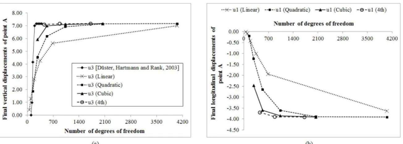
6.2 Cantilever beam under free-end shear force

The second example is a prismatic cantilever beam under a shear force at the free end (see figure 3). The performance of the present finite element in an extreme bending situation is analyzed here. Due to the symmetry regarding the plane

x

(11)

ele-Latin American Journal of Solids and Structures 10(2013) 1177 – 1209

ments and approximation orders have been employed. The final vertical displacement of point A (see figure 3) converges to the reference solution (see figure 4a) for all the approximation orders. However, as expected, for the linear and quadratic elements a large number of degrees of freedom are necessary to reach convergence of displacements, and the cubic and fourth-order elements are capable of simulating this problem with few degrees of freedom (see figures 4a and 4b). In the reference [3] shell-like solid finite elements of high-order (from one to eight) are employed, and convergence analysis is also carried out. Regarding the reference solution presented here (see fig-ure 4a), the number of solid finite elements is two: one with dimensions 0.10 x 0.10 x 0.10 close to the clamped section, and other with dimensions 9.9 x 0.10 x 0.10. In addition, the orders of poly-nomial approximation in [3] are four in the in-plane directions, and variable (from one to eight) in the beam thickness direction.

Figure 3 Cantilever beam under free-end shear force: geometry, boundary conditions and material parameters. The dashed lines denote the discretized part of the cantilever.

Figure 4 Cantilever beam under free-end shear force: (a) study of convergence regarding the final vertical displacements of point A; (b) study of convergence regarding the final longitudinal displacements of point A. The word in parenthesis is the approximation order

of the elements.

6.3 Cook’s m em brane

(12)

has six shell-like solid finite elements of variable order. The results in terms of displacements and stresses are in accordance with [3] (see figures 6a-c). The reference value in figure 6a corresponds to the converged solution, and the reference values in figures 6b and 6c have been obtained by meshes with linear approximation along the thickness direction and variable order (from one to seven) in the in-plane directions. As one can see, the linear elements of the present formulation present severe locking, and the cubic and fourth-order elements present fast convergence to the solution. The expressions employed to obtain the Euclidean norm of the displacement and the equivalent Cauchy stress are:

2 2 2 2

i 1 2 3

ue

₌

u

₌

u

₊

u

₊

u

₍₃₄₎

teq

₌

3

2 dev

σ

_{: dev}

σ

₌

3

2 dev

σ

(

)

_ij

(

dev

σ

)

ij (35)

where

u

i is the displacement along direction

x

_i;

dev

( )

denote the deviator operator; and

σ

is

the Cauchy stress tensor. One can note the singularity at point C as the final equivalent Cauchy stresses do not converge clearly with mesh refinement (see table 1). The final configuration of one of the meshes is depicted in figure 6d, in which one can see the complexity of the displacement field around point C. It is important to note that if the linear hyperelastic Saint Venant-Kirchhoff model is adopted to run this problem, material annihilation occurs even for low values of the ap-plied load.

6.4 T hin cylinder under tw o opposite line forces

(13)

(14)

Figure 6 Cook’s membrane: (a) study of convergence regarding the final displacements of point A; (b) study of convergence regard-ing the final Euclidean norm (34) at point A; (c) study of convergence regardregard-ing the final equivalent Cauchy stress (35) at point D;

(d) final displacements along direction

_x

2 (general view and zoom around point C). The symbols

u2

and

ue

(b) are, respectively,

the displacement of point A along direction

x

2 and the Euclidean norm (34) of the point A displacement. The results showed in (d) are provided by the mesh with 361 nodes (2527 degrees of freedom) and 72 shell elements of cubic order.

The dashed lines denote the membrane discretization.

Table 1 Final stresses at point C for the Cook’s membrane (see figure 5).

ORD NN NDOF NE σ₁₁ τ₁₂ teq

1

20 140 24 73.057 0.557 219.039 63 441 96 296.104 0.954 891.253 130 910 216 538.331 0.742 1618.384 3185 22295 6144 69.718 0.949 212.388

2

63 441 24 -12.247 0.376 34.940 221 1547 96 7.976 0.593 28.196 475 3325 216 -0.989 0.710 4.297 1089 7623 512 9.383 0.732 32.149

3 130 910 24 -17.058 0.654 46.246 361 2527 72 10.013 0.596 35.572 4 221 1547 24 -35.404 0.808 99.518

ORD = finite element order. NN = number of nodes. NDOF = number of degrees of freedom.

NE = number of elements. σ_{11 = normal stress along x1-direction.}τ_{12 = shear stress on the}

plane x1-x2. teq = equivalent stress (equation 35).

(15)

Figure 8 Thin cylinder under two opposite line forces: (a) convergence study regarding the final vertical displacement of point A; (b) final vertical displacements for the mesh with 6601 nodes (46207 degrees of freedom) and 800 fourth-order elements. The words in the

(16)

6.5 T hin plate ring

The thin clamped plate ring under a uniformly distributed shear force at the free edge, depicted in figure 9, is analyzed here. This numerical example is a benchmark shell problem often studied in the scientific literature (see, for example, [31], [26], [36], [37] and [24]). This problem is used to identify shear locking in the thin-shell limit for bending dominated situations. The hyperelastic model and the material parameters are extracted from [24], who employed a mixed isoparametric tri-linear brick finite element together with an enhanced assumed strain formulation for finite deformations to avoid locking problems. Regarding the final vertical displacement of point A, the results of the present cubic and fourth-order elements converge better than the reference finite element results, however the shell elements of linear degree present severe locking even for a large number of degrees of freedom (see figure 10a). The final deformed configuration, for the most refined mesh, is illustrated in figure 10b.

Figure 9 Thin plate ring: geometry, boundary conditions and constitutive law.

Figure 10 Thin plate ring: (a) (b) study of convergence regarding the final vertical displacement of point A; (b) final vertical dis-placements for the mesh with 1737 nodes (12159 degrees of freedom) and 192 finite elements of fourth-order. The words in the graph

(17)

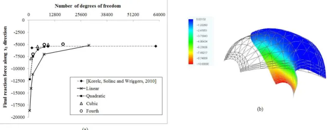
6.6 Spherical shell

The present numerical example is the spherical shell with an 18˚ hole, showed in figure 11. This benchmark shell problem is similar to the hemispherical shell with an 18˚ hole, which is usually employed to validate shell finite element formulations (see, for example, [26,31,36-38]). Geometry data, constitutive law and boundary conditions are the same as those used in [24]. Due to the symmetry regarding the planes

x

1

=

0.0

,

x

2

=

0.0

and

x

3

=

0.0

(see figure 11), only one eighth

of the shell is discretized. As pointed out by [24], this test can show if the numerical formulation exhibits shear locking in doubled-curved shell elements under large rotations. Again, the numeri-cal results of this study converge to the reference solution (see figure 12a). The final equilibrium configuration, for the most refined mesh, is depicted in figure 12b.

Figure 11 Spherical shell with an 18˚ hole: geometry, boundary conditions and material coefficients.

Figure 12 Spherical shell with an 18˚ hole: (a) study of convergence regarding the reaction force along the

x

3 direction; (b) final

(18)

6.7 Pinched cylinder w ith rigid diaphragm s

According to [27], this benchmark problem is similar to a finger-pinched beer can (see figure 13). Usually, the constitutive law employed to simulate this numerical example is the linear Saint Venant-Kirchhoff hyperelastic model (see [26,27,31,37,39], among many others). Here the adopted hyperelastic model is the nonlinear neo-Hookean law (18). The material coefficients have been found via the following transformations:

k

₌

E

3 1

(

−

2 ν

)

(36)

µ =

E

2 1

(

+

ν

)

(37)

where

E

and

ν

_{are the Young modulus and the Poisson’s ratio, respectively. To analyze this}

pinched cylinder with the Saint Venant-Kirchhoff model, the usual material coefficients are

E

₌

30000.0

_and

ν

₌

0.30

_{. Due to the symmetry regarding the planes}

x

1

=

100.0

,

x

2

=

0.0

and

x

3

=

0.0

, only one eighth of the cylinder is discretized. As the resultant displacement field is

complex and there may be structural instabilities, two large numbers of finite elements have been adopted: 512 (16 x 16 x 2) and 1152 (24 x 24 x 2). Again, locking regarding the vertical reaction force can be avoided with mesh refinement (see figure 14a). Small differences between the present and the reference numerical solutions were expected as the adopted constitutive models are differ-ent, and these differences increase with an increasing applied force (see figure 14b). The reference solution has been obtained with 1600 (40 x 40) 4-node hybrid stress and enhanced strain shell finite elements [31]. For the most refined mesh, the final deformed configuration of the cylinder is depicted in figure 14c.

(19)

Figure 14 Pinched cylinder with rigid diaphragms: (a) study of convergence regarding the applied force along the

_x

2 direction; (b) applied vertical force versus displacements (reference and present numerical solutions); (c) final vertical displacements for the mesh with 9409 nodes (65863 degrees of freedom) and 1152 finite elements of fourth-order. The words in the graph caption (a) correspond

to the element approximation degree.

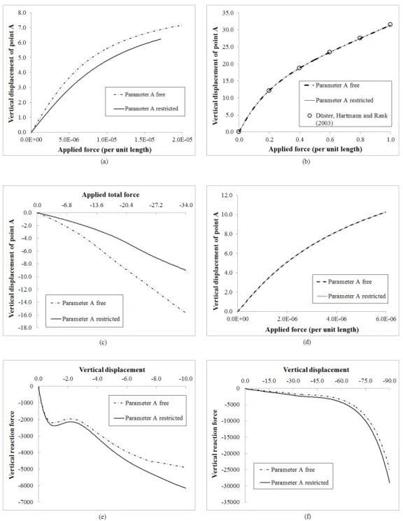
6.8 Shell finite elem ent w ith six nodal param eters

(20)

is very small. The final distribution of the seventh parameter “a”, for some examples, is depicted in figure 18, in which one can see that, although the restriction of this parameter has a clear in-fluence on the structural behavior (see figures 15-17), the final value of “a” is very small when compared to the unit (except for the region around the applied force on the pinched cylinder).

Figure 15 Influence of the seventh nodal parameter: (a) applied force versus vertical displacement of point A for the cantilever of figure 3; (b) applied force versus vertical displacement of point A for the Cook’s membrane of figure 5; (c) applied force versus vertical

displacement of point A for the thin cylinder of figure 7; (d) applied force versus vertical displacement of point A for the thin plate ring of figure 9; (e) reaction force versus prescribed displacement for the spherical shell of figure 11; (f) reaction force versus

(21)

Table 2 Meshes employed in order to show the influence of the seventh nodal parameter “a” on the finite element solution.

Problem (item) ORD NN NDOF NE NNIP

Plane ξ₁-ξ₂ Direction ξ₃

Cantilever (6.2) 4 485 3395 48 19 2

Cook's membrane (6.3) 4 221 1547 24 19 2

Thin cylinder (6.4) 4 6601 46207 800 19 2

Ring plate (6.5) 4 1737 12159 192 19 2

Spherical shell (6.6) 4 2401 16807 288 19 2

Pinched cylinder (6.7) 4 9409 65863 1152 19 2

ORD = shell finite element order. NN = number of nodes. NDOF = number of degrees of freedom.

NE = number of finite elements. NNIP = number of numerical integration points.

Figure 16 Distributions for the cantilever of figure 3 along the line segment

(

x₁₌0.01, x₂₌0.0,₋0.05_≤x₃_≤0.05

)

: (a)

(22)

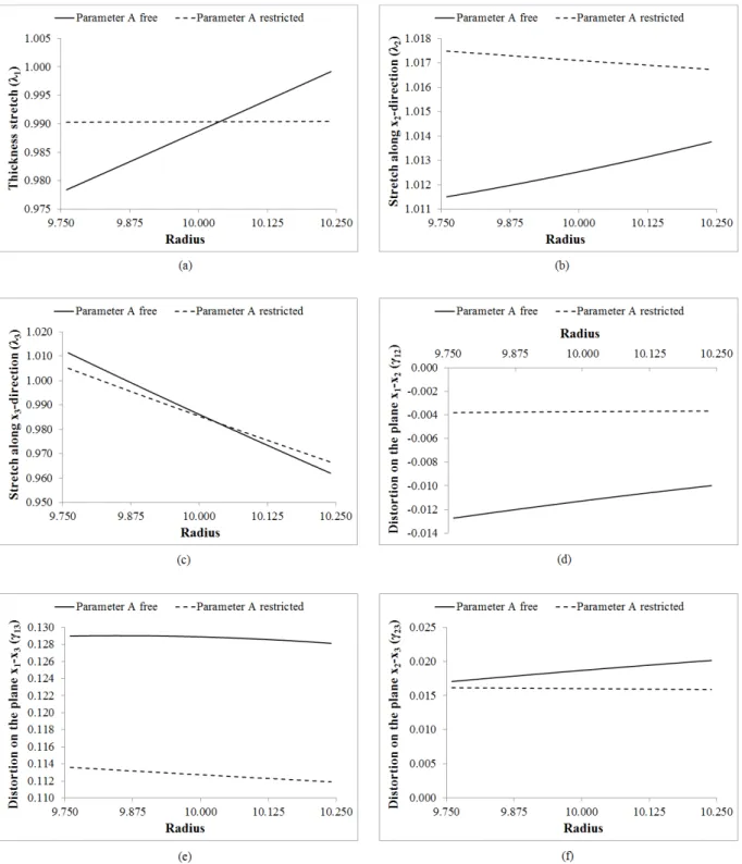
Figure 17 Final distributions for the spherical shell of figure 11 along the thickness direction at point C: (a) thickness stretch; (b) stretch along x2-direction; (c) stretch along x3-direction; (d) distortion on plane x1-x2; (e) distortion on plane x1-x3; (f) distortion on

(23)

Figure 18 Final distribution of the seven parameter “a”: (a) cantilever beam of figure 3; (b) thin cylinder of figure 7; (c) spherical shell of figure 11; (d) pinched cylinder of figure 13. The meshes employed here are given in table 2.

Another comparison has been performed in order to show the influence of the seventh parameter “a” and the Poisson’s ratio on the behavior of the pinched cylinder of figure 13. It is well known that values of Poisson’s ratio close to 0.50 leads to locking problems. So, besides the first value

ν

₌

0.30

_{, two more values have been selected:}

ν

₌

0.45

_and

ν

₌

0.49

_{. As the hyperelastic}

(24)

The results of the present section reinforce the importance of modeling the linear variation of strain along the thickness direction for shells with large displacements whose material behavior is described by nonlinear hyperelastic laws.

Figure 19 Influence of Poisson coefficient and parameter “a” on the behavior of the pinched cylinder of figure 13: (a) displacement of point A along direction x2; (b) displacement of point B along direction x3. These results correspond to the mesh with 9409 nodes

(65863 degrees of freedom) and 1152 shell finite elements of fourth-order. The simulation with the parameter “a” restricted and ν₌0.49_{has collapsed for a vertical displacement of point A equal to -65.5.}

7 C O N C LU SIO N S

(25)

Latin American Journal of Solids and Structures 10(2013) 1177 – 1209 References

[1] H. Hakula, Y. Leino and J. Pitkäranta. Scale resolution, locking, and high-order finite ele-ment modelling of shells. Comput. Methods Appl. Mech. Engrg., 133: 157-182, 1996.

[2] M. Suri. Analytical and computational assessment of locking in the hp finite element method.

Comput. Melhods Appl. Mech. Engrg., 133: 347-371, 1996.

[3] A. Düster, S. Hartmann and E. Rank. p-FEM applied to finite isotropic hyperelastic bodies.

Comput. Methods Appl. Mech. Engrg., 192: 5147-5166, 2003.

[4] J.N. Reddy. Mechanics of laminates composite plates and shells: theory and analysis. Boca Raton : CRC Press, 2004.

[5] R.A. Arciniega and J.N. Reddy. Large deformation analysis of functionally graded shells.

International Journal of Solids and Structures, 44: 2036-2052, 2007.

[6] Y. Basar, U. Hanskötter and Ch. Schwab. A general high-order finite element formulation for shells at large strains and finite rotations. Int. J. Numer. Meth. Engng., 57: 2147-2175, 2003.

[7] C.S. Jog. Higher-order shell elements based on a Cosserat model, and their use in the topolo-gy design of structures. Comput. Methods Appl. Mech. Engrg., 193: 2191-2220, 2004.

[8] E. Rank, A. Düster, V. Nübel, K. Preusch and O.T. Bruhns. High order finite elements for shells. Comput. Methods Appl. Mech. Engrg., 194: 2494-2512, 2005.

[9] H.B. Coda and R.R. Paccola. A positional FEM Formulation for geometrical non-linear analysis of shells. Latin American Journal of Solids and Structures, 5: 205-223, 2008.

[10] G.M. Kulikov and E. Carrera. Finite deformation higher-order shell models and rigid-body motions. International Journal of Solids and Structures, 45: 3153-3172, 2008.

[11] J.C. Simo, M.S. Rifai and D.D. Fox. On a stress resultant geometrically exact shell model. Part IV: variable thickness shells with through-the-thickness stretching. Comput. Methods Appl. Mech. Engrg., 81: 91-126, 1990.

[12] Y. Basar and Y. Ding. Finite-element analysis of hyperelastic thin shells with large strains.

Computational Mechanics, 18: 200-214, 1996.

(26)

[14] N. Büchter and E. Ramm.3d-extension of nonlinear shell equations based on the enhanced assumed strain concept. In: Hirsch, C. (Ed.), Computational Methods in Applied Sciences. Elsevier, Amsterdam, pp. 55-62.

[15] J. Bonnet, H. Marriott and O. Hassan. An averaged nodal deformation gradient linear tetra-hedral element for large strain explicit dynamic applications. Commun. Numer. Meth. Engng., 17: 551-561, 2001.

[16] H.B. Coda and M. Greco. A simple FEM formulation for large deflection 2D frame analysis based on position description. Comput. Methods Appl. Mech. Engrg., 193: 3541-3557, 2004.

[17] R.W. Ogden. Non-linear Elastic Deformations. Ellis Horwood Ltd., Chichester, England, 1984.

[18] M.A. Crisfield. Non-linear Finite Element Analysis of Solids and Structures. John Wiley & Sons, Chichester, England, 2000.

[19] G.A. Holzapfel. Nonlinear Solid Mechanics - A Continuum Approach for Engineering. John Wiley & Sons Ltd., Chichester, England, 2004.

[20] O.H. Yeoh, Hyperelastic Material Models for Finite Element Analysis of Rubber. J. Nat. Rubb. Res., 12: 142-153, 1997.

[21] S. Hartmann and P. Neff. Polyconvexity of generalized polynomial-type hyperelastic strain energy functions for near-incompressibility. International Journal of Solids and Structures, 40: 2767-2791, 2003.

[22] K.Y. Sze, S.J. Zheng and S.H. Lo. A stabilized eighteen-node solid element for hyperelastic analysis of shells. Finite Elements in Analysis and Design, 40: 319-340, 2004.

[23] J.P. Pascon. Modelos constitutivos para materiais hiperelásticos: estudo e implementação computacional. Master’s dissertation. São Carlos: Departamento de Engenharia de Estru-turas, EESC, USP, 2008.

[24] J. Korelc, U Solinc and P. Wriggers. An improved EAS brick element for finite deformation.

Comput. Mech., 46: 641-659, 2010.

(27)

[26] E.M.B. Campello, P.M. Pimenta and P. Wriggers. A triangular finite shell element based on a fully nonlinear shell formulation. Computational Mechanics, 31: 505-518, 2003.

[27] P.M. Pimenta, E.M.B. Campello and P. Wriggers. A fully nonlinear multi-parameter shell model with thickness variation and a triangular shell finite element. Computational Mechan-ics, 34: 181-193, 2004.

[28] N. Büchter, E. Ramm and D. Roehl. Three-dimensional extension of non-linear shell formu-lation based on the enhanced assumed strain concept. International Journal for Numerical Methods in Engineering, 37: 2551-2568, 1994.

[29] H. Parisch. A continuum-based shell theory for non-linear applications. International Journal for Numerical Methods in Engineering, 38: 1855-1883, 1995.

[30] N. El-Abbasi and S.A. Meguid. A new shell element accounting for through-thickness defor-mation. Comput. Methods Appl. Mech. Engrg., 189: 841-862, 2000.

[31] C. Sansour and F.G. Kollmann. Families of 4-node and 9-node finite elements for a finite deformation shell theory. An assesment of hybrid stress, hybrid strain and enhanced strain elements. Computational Mechanics, 24: 435-447, 2000.

[32] G.R. Cowper. Gaussian quadrature formulas for triangles. International Journal for Numeri-cal Methods in Engineering, 7: 405-408, 1973.

[33] J. N. Lyness and D. Jespersen. Moderate degree symmetric quadrature rules for the triangle.

J. Inst. Maths. Applics., 15: 19-32, 1975.

[34] D.A. Dunavant. High degree efficient symmetrical Gaussian quadrature rules for the triangle.

International Journal for Numerical Methods in Engineering, 21: 1129-1148, 1985.

[35] I.S. Duff. MA57 - A Code for the Solution of Sparse Symmetric Definite and Indefinite Sys-tems, 2004.

[36] A. Petchsasithon and P. D. Gosling. locking-free hexahedral element for the geometrically non-linear analysis of arbitrary shells. Comput Mech, 35: 94-114, 2005.

[37] H.B. Coda and R.R. Paccola. An alternative positional FEM formulation for geometrically non-linear analysis of shells: curved triangular isoparametric elements. Comput Mech, 40: 185-200, 2007.

(28)

[39] K.Y. Sze, X.H. Liu and S.H. Lo. Popular benchmark problems for geometric nonlinear analy-sis of shells. Finite Elements in Analysis and Design, 40: 1551-1569, 2004.

A ppendix A - Shape functions coefficients

The expressions for determination of the matrices

M

coef,

Md1

and

Md 2

, and the vectors

v

ξ,

v

ξ1 and

v

ξ2 (see equations 31-33) are provided here.

For a two-dimensional triangular finite element of polynomial order p, the number of nodes per element is:

(

)(

)

1 nnpe

p 1 p

2

2 =

+

(A1)

The internal numbering of the nodes - or the numbering of the nodes inside each element do-main - is depicted in figure A1. The general expressions employed here to determine the non-dimensional coordinates

ξ

₁ and

ξ

₂ of the nodes for any element order are provided in table A1. One can note that, regarding the non-dimensional auxiliary space, the nodes with the same coor-dinate

ξ

1 or

ξ

2 are equally spaced.

Figure A1 Internal numbering of the nodes for a general two-dimensional triangular finite element. The symbols

ξ

1 and

ξ

2 are the

(29)

Table A1 Determination of the non-dimensional coordinates

ξ

1 and

ξ

2 for the triangular finite element of figure A1.

For any isoparametric triangular finite element of order p, all the shape functions can be written via the following general polynomial expression:

φ

k

( )

ξ

=

c

0 k

+

c

1 k

ξ

1

+

c

2 k

ξ

2

+

c

3 k

ξ

1 2

+

c

4 k

ξ

1

ξ

2

+

c

5 k

ξ

2 2

+

c

6 k

ξ

1 3

+

c

7 k

ξ

1 2

ξ

2

+

c

8 k

ξ

1

ξ

2 2

+

c

9 k

ξ

2 3

+

...

₊

c

₍k_nnpe−3₎

ξ

₁2

_ξ

2 p−2

+

c

₍k_nnpe−2₎

ξ

₁

ξ

₂p−1

+

c

₍k_nnpe−1₎

ξ

₂p (A2)

where

c

n k

is the n-th coefficient of the shape function associated with node k. Expression (A2) can be rewritten in an alternative way:

φ

₁

φ

₂

φ

₃

φ

₄

φ

₅

φ

₆



φ

_nnpe

⎧

⎨

⎪

⎪⎪

⎩

⎪

⎫

⎬

⎪

⎪⎪

⎭

⎪

=

c

1₀

c

₁1

c

1₂

c

1₃

c

1₄

c

₅1



_c

nnpe−1 1

c

₀2

c

₁2

c

₂2

c

₃2

c

₄2

c

₅2



_c

nnpe−1 2

c

₀3

c

₁3

c

₂3

c

₃3

c

3₄

c

₅3



_c

nnpe−1 3

c

₀4

c

₁4

c

₂4

c

₃4

c

₄4

c

₅4



_c

nnpe−1 4

c

₀5

c

₁5

c

₂5

c

₃5

c

5₄

c

₅5



_c

nnpe−1 5

c

₀6

c

₁6

c

₂6

c

₃6

c

6₄

c

₅6



_c

nnpe−1 6







c

₀nnpe

c

₁nnpe

c

₂nnpe

c

₃nnpe

c

₄nnpe

c

₅nnpe



_c

nnpe−1 nnpe

⎡

⎣

⎢

⎤

⎦

⎥

1 ξ

₁

ξ

₂

ξ

₁2

ξ

₁

ξ

₂

(30)

This expression is the expanded form of equation (31). In order to determine the matrix of coeffi-cients

Mcoef

, one uses the property of the Lagrange polynomials:

Φ

_i

_{( )}

ξ

_k

=

(

M

_coef

)

ij

⎡

⎣

v

ξ

( )

ξ

k

⎤

⎦

j

=

δ

ik (A4)

where

Φ

_i

( )

ξ

_k and

⎡

_⎣

v

_ξ

( )

ξ

_k

⎤

_⎦

j are the values of the shape function

Φ

i and the vector component

v

_ξ

( )

_j at node k; and

δ

ik is the Kronecker delta. Expanding equation (A4):

φ₁

( )

ξ₁ φ₁

( )

ξ₂ φ₁

( )

ξ₃ φ₁

( )

ξ₄ φ₁

( )

ξ₅ φ₁

( )

ξ₆  φ

1

(

ξnnpe

)

φ₂

( )

ξ₁ φ₂

( )

ξ₂ φ₂

( )

ξ₃ φ₂

( )

ξ₄ φ₂

( )

ξ₅ φ₂

( )

ξ₆  φ

2

(

ξnnpe

)

φ₃

( )

ξ₁ φ₃

( )

ξ₂ φ₃

( )

ξ₃ φ₃

( )

ξ₄ φ₃

( )

ξ₅ φ₃

( )

ξ₆  φ

3

(

ξnnpe

)

φ

4

( )

ξ1 φ4

( )

ξ2 φ4

( )

ξ3 φ4

( )

ξ4 φ4

( )

ξ5 φ4

( )

ξ6  φ4

(

ξnnpe

)

φ

5

( )

ξ1 φ5

( )

ξ2 φ5

( )

ξ3 φ5

( )

ξ4 φ5

( )

ξ5 φ5

( )

ξ6  φ5

(

ξnnpe

)

φ₆

( )

ξ₁ φ₆

( )

ξ₂ φ₆

( )

ξ₃ φ₆

( )

ξ₄ φ₆

( )

ξ₅ φ₆

( )

ξ₆  φ

6

(

ξnnpe

)

       

φ_nnpe

( )

ξ₁ φ_nnpe

( )

ξ₂ φ_nnpe

( )

ξ₃ φ_nnpe

( )

ξ₄ φ_nnpe

( )

ξ₅ φ_nnpe

( )

ξ₆  φ

nnpe

(

ξnnpe

)

⎡

⎣

⎢

⎤

⎦

⎥

=

c01 c11 c21 c31  _cnnpe−11

c02 c12 c22 c32  _cnnpe−12

c03 c13 c23 c33  _cnnpe−13

c04 c14 c24 c34  _cnnpe−14

     

c0nnpe c1nnpe c2nnpe c3nnpe  _cnnpe−1nnpe

⎡ ⎣ ⎢ ⎢ ⎢ ⎢ ⎢ ⎢ ⎢ ⎢ ⎤ ⎦ ⎥ ⎥ ⎥ ⎥ ⎥ ⎥ ⎥ ⎥

1 1 1 1  1

ξ_{1 1}

( )

ξ_{1 2}

( )

ξ_{1 3}

( )

ξ_{1 4}

( )

 ξ

1 nnpe

(

)

ξ_{2 1}

( )

ξ_{2 2}

( )

ξ_{2 3}

( )

ξ_{2 4}

( )

 ξ

2 nnpe

(

)

ξ_{1 1}

( )

2 ξ_{1 2}

( )

2 ξ_{1 3}

( )

2 ξ_{1 4}

( )

2  ξ

1 nnpe

(

)

2

     

ξ_{2 1}

( )

p ξ_{2 2}

( )

p ξ_{2 3}

( )

p ξ_{2 4}

( )

p  ξ

2 nnpe

(

)

p ⎡ ⎣ ⎢ ⎢ ⎢ ⎢ ⎢ ⎢ ⎢ ⎤ ⎦ ⎥ ⎥ ⎥ ⎥ ⎥ ⎥ ⎥ =I

or 1

coef ξ coef ξ

−

=

⇒

₌

M

I

M

(A5)

where

ξ

₁

( )

_k

and

ξ

₂

( )

_k

are the non-dimensional coordinates of node k;

I

is the identity matrix. As one can see, the matrix that contains the coefficients of all the shape functions is easily found via a simple matrix inversion. The determination of the matrix

M

ξ and the vector

v

ξ, for any

(31)

Table A2 Determination of the matrix

_Mξ

(see expressions A5 and A6) for finite element of figure A1.

Table A3 Determination of the vector

v

_ξ (see expressions 31 and A3) for any point P inside the domain of the element depicted in

(32)