Economia Aplicada, v. 18, n. 1, 2014, pp. 51-67
THE FREQUENCY DOMAIN CAUSALITY ANALYSIS
BETWEEN ENERGY CONSUMPTION AND INCOME IN
THE UNITED STATES
Aviral Kumar Tiwari*
Abstract
We investigated Granger-causality in the frequency domain between primary energy consumption/electricity consumption and GDP for the US by employing approach of Lemmens et al. (2008) and covering the period of January, 1973 to December, 2008. We found that causal and re-verse causal relations between primary energy consumption and GDP and electricity consumption and GDP vary across frequencies. Our unique contribution in the existing literature lies in decomposing the causality on the basis of time horizons and demonstrating bidirectional the short-run, the medium-run and the long-run causality between GDP and primary en-ergy consumption/electricity consumption and thus providing evidence for the feedback hypothesis. These results have important implications for the US for planning of the short, the medium and the long run energy and economic growth related policies.
Keywords:Energy consumption; Economic growth; Granger-causality in the frequency domain.
Resumo
Através do teste de casualidade de Granger, nós investigamos o domí-nio de frequência entre o consumo primário de energia/eletricidade e o produto interno bruto (PIB) dos Estados Unidos; aplicando a abordagem de Lemmens et al. (2008) e cobrindo o período entre Janeiro de 1973 a De-zembro de 2008. Nós achamos relações causal e causal reversa entre o con-sumo primário de energia e PIB, e o concon-sumo de eletricidade e PIB variam através das frequências. Nossa contribuição única na literatura existente reside na decomposição da causalidade com base em horizontes de tempo e demonstração bi-direcional de causalidade de curto prazo, médio-prazo e longo-prazo entre PIB e consumo primário de energia/eletricidade e as-sim provendo evidência para a “feedback hypothesis”. Estes resultados têm importantes implicações para o planejamento energértico de curto, médio e longo prazo dos Estados Unidos e políticas relacionadas ao cres-cimento econômico.
Palavras-chave:Consumo de Energia; Crescimento Econômico; Granger-Casualidade no Domínio da Frequência.
JEL classification:Q40, Q43, Q53, Q56.
DOI:http://dx.doi.org/10.1590/1413-8050/ea307
*Research scholar and Faculty of Applied Economics, Faculty of Management, ICFAI University
Tripura. E-mail: [email protected]
52 Tiwari Economia Aplicada, v.18, n.1
1
Introduction
Voluminous studies have examined the relationship between energy consump-tion and economic growth and suggested policy implicaconsump-tions derived from their empirical findings. This line of inquiry stems basically, from the earlier oil shocks of the 1970s to the more recent interest in energy prices and the impact of the Kyoto protocol agreement by a number of industrialized and developing countries to conserve energy and reduce greenhouse emissions in the face of achieving high growth rate of the economies. Economic theories, al-though, provide an unambiguous relationship between energy consumption, and economic growth (see section 2), the empirical investigation of the rela-tionship between these variables has been one of the most attractive areas of energy economics literature for the last two decades. In recent years, there has been a renewed interest in examining the relationship between these vari-ables. The high economic growth rates experienced by developing countries are achievable only with the consumption of a larger quantity of commercial energy, which is one of the key factors of production, though it leads to envi-ronmental degradation. There is still dispute on whether energy consumption is a stimulating factor for, or a result of, economic growth. In this we study reinvestigate the same issue but used a recent frequency domain approach de-veloped by Lemmens et al. (2008), thus making a novel contribution to the research on the existing literature examining the relationship between energy consumption and economic growth. Our results have supported the findings of Yang (2000) for Taiwan, Zachariadis & Pashourtidou (2007) for Cyprus, Tang (2008) and Lean & Smyth (2010) for Malaysia, Aktas & Yilmaz (2008)
for Turkey, Odhiambo (2009a) for South Africa, Lorde et al. (2010) for
Barba-dos, Ouédraogo (2010) for Burkina Faso, Tiwari (2010) for India and Shahbaz et al. (2011) for Portugal.
We focus on the United States (US) because of the important role that it plays in world energy markets. Soytas et al. (2007) make some observations regarding this. ‘First, according to the Statistical Abstract of the US (2006), GHG emissions in the US rose nearly 17% between 1990 and 2000 before
leveling off in 2001 and 2002. Second, over that same time period, the US
accounted for around 23 to 24% of the world’s total CO2emissions from
con-sumption of fossil fuels. Third, the US share of total world energy produc-tion has fallen slightly from 20% in 1990 to 18% and 17% in the years 2000 and 2003, respectively. Fourth, over the same time frame, the US share of total world energy consumption has remained fairly constant at around 24%’. These facts confirm that the US is a significant consumer, as well as producer, of energy in the world economy. Therefore, it is important to better under-stand the relationships that exist between US economic growth and energy
use before effective policies are developed.
The issue of the possible impact of CO2emissions reduction on economic
growth inevitably arises due to the possible connection between CO2
emis-sions and energy consumption, and energy consumption and economic growth. As a result of the importance of the possible connection between energy con-sumption and economic growth, literature is increasing in this area. In gen-eral, studies find evidence of correlation between these two variables for
coun-tries with different economic structures and different stages of economic
The Frequency Domain Causality analysis between Energy Consumption 53
the Granger-causality (GC) test to US data for the period of 1947-1974, and found that a unidirectional causality runs from economic growth to energy consumption, thus suggesting that an energy conservation policy is feasible. Since Kraft & Kraft (1978), there has been a vast body of studies contributing to this literature. Table 1 summarizes related studies.
Our observation from Table 1 indicates that studies in this area have pro-duced mixed and often conflicting results for both developed and developing
countries due to different methods, sample periods, and model specifications
being employed. Furthermore, it is worth noting that most previous studies are limited in scope to the applications of linear models. However, economic events and regime changes such as changes in economic environment, in en-ergy policy and fluctuations in enen-ergy price can cause structural alterations in the pattern of energy consumption for a given time period under study. This creates a room for a nonlinear rather than linear relationship between energy consumption and economic growth. Therefore, in the present study we made an attempt to analyze the issue in a nonlinear framework by using a recently developed nonparametric approach of Lemmens et al. (2008). Use of this approach allows us to decompose the GC in the frequency domain. In frequency domain, the key idea is that a stationary process can be described
as a weighted sum of sinusoidal components with a certain frequencyλ. As a
result, one can analyze these frequency components separately. This analysis will make it possible to determine whether the predictive power is concen-trated at the quickly fluctuating components or at the slowly fluctuating com-ponents. As such, instead of computing a single GC measure for the entire relationship, the GC is calculated for each individual frequency component
separately. Thus, the strength and/or direction of the GC can be different
for each frequency. In the present we study have considered two measures of energy consumption namely, primary energy consumption and electricity consumption. Two measures of energy consumption have been used to ob-serve the robustness of our results. To the best of our knowledge, the analyses of GC from primary energy consumption and/or electricity consumption to economic growth and vice-versa have not yet been explored in the frequency
domain.1
The next section discusses the hypothesis data source and methodology. Section three presents empirical findings and section four draws conclusions and policy implications.
2
Hypotheses, Data Source and Methodology
The direction of causality between the energy consumption and economic growth has important policy implications as to whether an energy
conser-1It is important to mention that our analysis is based on the bivariate Granger causality
anal-ysis model and therefore, suffers from the problem of omitted variable bias. However, we would
argue that even if this is the first case, to the best of our knowledge there is no such test developed which analyses nonlinear Granger-causality in a multivariate framework (the only exception ne-gin is Breitung & Candelon (2006) which can be applied for, at the most, a trivariate model. However, here we have preferred the test suggested by Lemmens et al. (2008) which is relatively more suitable vis-à-vis Breitung & Candelon (2006) proposed test). Second, since the approach used in the study is based on a nonlinear framework, we would argue that if any omitted variable
is able to transmit its effect on the measured variable and create nonlinearity in the data series,
we are able to take care of the effect of those variables in our analysis through the approach we
5
4
T
iw
ar
i
E
co
no
m
ia
A
pli
ca
da
,v
.1
8,
n.1
Table 1: Summary of Literature on Relationship between Electricity Consumption and Economic Growth
Authors Time Period Methodology Variables Cointegration Findings (country studied)
Single-Country Studies
Yang (2000) 1954-1997 GC Real GDP and Electricity Consumption No EC↔Y (Taiwan)
Aqeel & Butt (2001) 1955-1996 GC by Hsiao Real GDP and Electricity Consumption No EC→Y(Pakistan)
Ghosh (2002) 1950-1997 JML, GC Electricity Supply, Employment and RealGDP Yes ES←Y(India)
Jumbe (2004) 1970-1999 GC, Real GDP and Electricity Consumption Yes EC←Y(Malawi)
Shiu & Lam (2004) 1971-2000 JML, VECM Real GDP and Electricity Consumption Yes EC→Y(China)
Lee & Chang (2005) 1954-2003 JML, VECM Real GDP per Capita and Electricity Con-sumption per Capita Yes EC→Y(Taiwan)
Narayan & Smyth (2005) 1966-1999 ARDL, VECM Real GDP per Capita, Electricity Consump-tion per Capita and Employment Yes EC←Y(Australia)
Yoo (2005) 1970-2002 JML, VECM Real GDP and Electricity Consumption Yes EC→Y(Korea)
Yoo & Kim (2006) 1971-2002 JML, GC by Hsiao Real GDP and Electricity Supply No ES←Y(Indonesia)
Ho & Siu (2006) 1966-2002 JML, VECM Real GDP and Electricity Consumption Yes EC→Y(Hong Kong)
Altinay & Karagol (2005) 1950-2005 GCDL Real GDP and Electricity Consumption N.A EC→Y(Turkey)
Yusaf & Latif (2007) 1980-2006 MJL, GC Real GDP and Electricity Consumption Yes EC↔Y(Malaysia)
Yuan et al. (2007) 1978-2004 JML, VECM Real GDP and Electricity Consumption Yes EC→Y(China)
Mozumder & Marathe (2007) 1971-1999 JML, VECM Real GDP per Capita, Electricity Consump-tion per Capita Yes EC←Y(Bangladesh)
Narayan & Singh (2007) 1971-2002 ARDL, VECM Real GDP, Electricity Consumption and La-bor Yes EC→Y(Fiji Islands)
Zachariadis & Pashourtidou (2007)
1960-2004 JML, VECM,
VARGFEVD
Real Income per Capita, Electricity Con-sumption, prices and weather
Yes EC↔Y(Cyprus)
Tang (2008) 1972-2003 ARDL, TYDL Gross National Product and Electricity Con-sumption No EC↔Y(Malaysia)
T
he
Fr
eq
ue
nc
y
D
om
ain
C
au
sa
lit
y
an
aly
sis
be
tw
ee
n
E
ne
rg
y
C
on
su
m
pt
io
n
5
5
Table 1: Summary of Literature on Relationship between Electricity Consumption and Economic Growth (continuação)
Authors Time Period Methodology Variables Cointegration Findings (country studied)
Single-Country Studies
Abosedra et al. (2009) 1995-2005 MJL, GC, VARGFEVD Real GDP, Electricity Consumption, Real Im-ports, Temperature and humidity No EC→Y(Lebanon)
Odhiambo (2009a) 1971-2006 JML, VECM Real GDP per Capita and Electricity Con-sumption per Capita, Employment Yes EC↔Y(South Africa)
Odhiambo (2009b) 1971-2006 ARDL, VECM Real GDP per Capita and Electricity Con-sumption per Capita Yes EC→Y(Tanzania)
Lean & Smyth (2010) 1971-2006 TYDL Real GDP, Electricity Consumption, Exports,Capita and Labor Yes EC↔Y(Malaysia)
Ciarreta & Zarraga (2010) 1971-2005 TYDL Real GDP and Electricity Consumption N.A EC←Y (Spain)
Lorde et al. (2010) 1960-2004 JML, VECM Real GDP, Electricity Consumption, Capital,Labor and Technology Yes EC↔Y(Barbados)
Acaravici (2010) 1968-2005 JML, VECM Real GDP and Electricity Consumption Existed EC→Y(Turkey)
Chandran et al. (2010) 1971-2003 ARDL, VECM Electricity consumption, Real GDP andPrices Yes EC→Y(Malaysia)
Jamil & Ahmad (2010) 1960-2008 VARGFEVDJML, VECM, Industrial Production, Electricity Consump-tion and Electricity Prices Yes EC↔Y(Pakistan)
Ouédraogo (2010) 1968-2003 ARDL, VECM Real GDP, Electricity Consumption and Cap-ital Formation Yes EC↔Y(Burkina Faso)
Tiwari (2010) 1971-2006 JJ, GC- TYDL Electricity consumption and Employment NA EC↔Y(India)
Shahbaz et al. (2011) 1971-2009 ARDL, GC-VECM Electricity consumption, economic growth,and employment Yes EC↔Y(Portugal)
Tiwari (2011a) 1971-2007 JJ, GC-VAR Real GDP per capita, Electricity consump-tion, CO2 emissions, Labor and Capital No EC↔Y(India)
Tiwari (2011b) 1970-2007 VAR, GC-DL Primary energy consumption, CO2 emis-sions, and economic growth No EC←Y(India)
Tiwari (2012) 1970-2005 Saikkonen and Lütke-pohl’s approach,
GC-VAR
CO2 emissions, energy consumption and economic growth
56 Tiwari Economia Aplicada, v.18, n.1
vation policy may or may not be adopted, depending on the direction of causality. Unidirectional causality running from GDP to energy consump-tion (EC) implies that income is the initial receptor of exogenous shocks and that equilibrium is restored through adjustment in EC. These are less energy dependent economies and energy conservation policies may be implemented
without adverse effects on economic growth and employment. On the other
hand, if causality runs from EC to GDP, it implies that the economy is energy dependent and EC measures may stimulate economic growth. Bidirectional causality indicates that both EC and a high level of economic activity mu-tually stimulate each other. Finally, no-causality between EC and economic growth referred as “neutrality hypothesis”, implies that energy conservation
measures may be pursued without affecting the economy.
For the analysis, we obtain data of primary energy consumption and elec-tricity consumption from the US Energy Information Administration (June 2011 Monthly Energy Review) with monthly observations. Data of real GDP is
obtained fromhttp://www.bea.doc.gov/with annual observations. In order to
match the observations, GDP data is interpolated using a linear interpolation
method, however, results are unaffected significantly if cubic interpolation is
used. Our study period is January, 1973 to December, 2008.2
Analysing time series in frequency domain i.e., spectral analysis, could be helpful in supplementing the information obtained by time-domain anal-ysis (Granger 1969, Priestley 1981). Spectral analanal-ysis highlights the cyclical properties of data. In our study, we follow the bivariate GC test over the spec-trum proposed by Lemmens et al. (2008). They have reconsidered the original framework proposed by Pierce (1979), and proposed a testing procedure for Pierce’s spectral GC measure. This GC test in the frequency domain relies
on a modified version of the coefficient of coherence, which they estimate in
a nonparametric fashion and for which they derive the distributional proper-ties.
LetEt andYt be two stationary time series of lengthT representing
En-ergy/ Electricity consumption and Output/GDP respectively. The goal is to
test whetherEtGranger causeYtat a given frequencyλ. Pierce’s measure for
GC (Pierce 1979) in the frequency domain is performed on the univariate
in-novations series,µt andνt, derived from filtering theEt andYtas univariate
ARMA processes, i.e.
ΘE(L)Et=CE+ΦE(L)ζt (1)
Θy(L)Yt=Cy+Φy(L)ξt (2)
2Here, we want to make clear that we have preferred to interpolate GDP instead of using
in-dustrial production data of which sufficient observations are available because first, interpolation
The Frequency Domain Causality analysis between Energy Consumption 57
whereΘE(L) andΘy(L) are autoregressive polynomials,ΦE(L) andΦy(L) are
moving average polynomials andCE andCy potential deterministic
compo-nents. The obtained innovation series ζt andξt, which are white-noise
pro-cesses with zero mean, possibly correlated with each other at different leads
and lags. The innovation seriesζt andξt, are the series of importance in the
GC test proposed by Lemmens et al. (2008).
LetSζ(λ) andSξ(λ) be the spectral density functions, or spectra, ofζtand
ξtat frequencyλ∈]0, π[, defined by
Sζ(λ) =
1
2π
∞
X
k−∞
γζ(k)e−iλk (3)
Sξ(λ) =
1
2π
∞
X
k−∞
γξ(k)e−iλk (4)
whereγζ(k) =Cov(ζt, ζt−k) andγξ(k) =Cov(ξt, ξt−k) represent the
autocovari-ances ofζtandξtat lagk. The idea of the spectral representation is that each
time series may be decomposed into a sum of uncorrelated components, each
related to a particular frequencyλ.3 The spectrum can be interpreted as a
decomposition of the series variance by frequency. The portion of variance of the series occurring between any two frequencies is given by area under the spectrum between those two frequencies. In other words, the area under
Sζ(λ) andSξ(λ), between any two frequenciesλ and λ+dλ, gives the
por-tion of variance ofζt andξt respectively, due to cyclical components in the
frequency band (λ, λ+dλ).
The cross spectrum represents the cross covariogram of two series in fre-quency domain. It allows determining the relationship between two time
se-ries as a function of frequency. LetSζξ(λ) be the cross spectrum betweenζt
andξtseries. The cross spectrum is a complex number, defined as,
Sζξ(λ) =Cζξ(λ) +iQζξ(λ)
1
2π
∞
X
k−∞
γζξ(k)e−λk
(5)
whereCζξ(λ) is called cospectrum andQζξ(λ) is called quadrature spectrum
are respectively, the real and imaginary parts of the cross-spectrum andi =
√
−1 . Hereγζξ(k) =Cov(ζt, ξt−k) represents the cross-covariance ofζtandξt
at lagk. The cospectrumQζξ(λ) between two seriesζt andξt at frequency
λcan be interpreted as the covariance between two seriesζt andξtthat is
at-tributable to cycles with frequencyλ. The quadrature spectrum looks for
evi-dence of out-of-phase cycles (see Hamilton 1994, pp.274). The cross-spectrum can be estimated non-parametrically by,
ˆ
Sζξ(λ) =
1
2π
M
X
k=−M
wkγˆζξ(k)e−iλk
(6)
3The frequenciesλ1, λ2, . . . , λ
Nare specified as follows:λ1= 2π/T , λ2= 4π/T , . . .. The highest
frequency considered isλN= 2N π/T; whereN≡T /2, ifTis an even number andN≡(T−1)/2,
58 Tiwari Economia Aplicada, v.18, n.1
with ˆγζξ =COVˆ (ζt, ξt−k) the empirical cross-covariances, and with window
weightswk, fork=−M, . . . , M. Equation (6) is called the weighted covariance
estimator, and the weightswk are selected as, the Bartlett weighting scheme
i.e. 1− |k|/M. The constant M determines the maximum lag order considered.
The spectra of Equation (3) and (4) are estimated in a similar way. This
cross-spectrum allows us to compute the coefficient of coherence hζξ(λ) defined
as,
hζξ(λ) = |
Sζξ(λ)|
p
Sζ(λ)Sξ(λ)
(7)
Coherence can be interpreted as the absolute value of a frequency specific
correlation coefficient. The squared coefficient of coherence has an
interpre-tation similar to the R-squared in a regression context. Coherence thus takes values between 0 and 1. Lemmens et al. (2008) have shown that, under the
null hypothesis that hζξ(λ) = 0, the estimated squared coefficient of
coher-ence at frequencyλ, with 0< λ < πwhen appropriately rescaled, converges to
a chi-squared distribution with 2 degrees of freedom,4denoted byχ2
2.
2 (n−1) ˆh2ζξ(λ)→dχ22 (8)
where →d stands for convergence in distribution, with n =T /PM
k=−Mw2k
.
The null hypothesishζξ(λ) = 0 versushζξ(λ)>0 is then rejected if
ˆ hζξ(λ)>
s χ22,1−α
2 (n−1) (9)
withχ22,1−α being the 1−αquantile of the chi-squared distribution with 2
de-grees of freedom. The coefficient of coherence in Equation (7) gives a measure
of the strength of the linear association between two time series, frequency by frequency, but does not provide any information on the direction of the relationship between two processes. Lemmens et al. (2008) have decomposed
the cross-spectrum (Equation 5) into three parts: (i)Sζ⇔⇒ξthe instantaneous
relationship betweenζtandξt; (ii)Sζ⇒ξ, the directional relationship between
ζtand lagged values ofξt; and (iii)Sζ⇒ξ, the directional relationship between
ξtand lagged values ofζt, i.e.,
Sζξ(λ) =
h
Sζ⇔⇒ξ+Sζ⇒ξ+Sξ⇒ζ
i 1 2π
γζξ(0) +
−1 X
k=−∞
γζξ(k)e−iλk+ ∞
X
k=1
γζξ(k)e−iλk
(10)
The proposed spectral measure of GC is based on the key property thatζt
does not Granger cause ξt if and only ifγζξ(k) = 0 for allk <0. The goal is
to test the predictive content ofζt relativeξt to which is given by the second
part of Equation (10), i.e.
Sζ⇒ξ(λ) =
1 2π −1 X
k=−∞
γζξ(k)e−iλk
(11)
4For the endpointsλ= 0 andλ=π, one only has one degree of freedom since the imaginary
The Frequency Domain Causality analysis between Energy Consumption 59
The Granger coefficient of coherence is then given by,
hζ⇒ξ(λ) =
Sζ⇒ξ(λ)
p
Sζ(λ)Sξ(λ)
(12)
Therefore, in the absence of GC, hζ⇒ξ(λ) = 0 for every λ in [0, π]. The
Granger coefficient of coherence takes values between zero and one, Pierce
(1979). Granger coefficient of coherence at frequencyλis estimated by
ˆ
hζ⇒ξ(λ) =
Sˆζ⇒ξ(λ)
q ˆ
Sζ(λ) ˆSξ(λ)
(13)
with ˆSζ⇒ξ(λ) as in Equation (6), but with all weightswk= 0 fork≥0. The
dis-tribution of the estimator of the Granger coefficient of coherence is derived
from the distribution of the coefficient of coherence Equation (8). Under
the null hypothesis ˆhζ⇒ξ(λ) = 0, the distribution of the squared estimated
Granger coefficient of coherence at frequencyλ, with 0< λ < πis given by,
2 (n′−1) ˆh2ζξ(λ)→dχ22 (14)
wherenis now replaced byn′=T /P−1
k=−Mwk2
. Since thewks′, with a positive
indexk, are set equal to zero when computing ˆSζ⇒ξ(λ), in effect only thewk
with negative indices are taken into account. The null hypothesis ˆhζ⇒ξ(λ) = 0
versus ˆhζ⇒ξ(λ)>0 is then rejected if
ˆ
hζ⇒ξ(λ)>
s χ22,1−α
2 (n′−1) (15)
Afterward, we compute Granger coefficient of coherence given be
Equa-tion (13) and test the significance of causality by making use of EquaEqua-tion (15).
3
Empirical Findings
First of all, we tested for the stationarity of the variables considered in our study through Phillips & Perron (1988) (PP) test, Kwiatkowski et al. (1992)
KPSS test and Zivot & Andrews (1992) (ZA) test.5 We report results of unit
root analysis in Table 2 below.
It is evident from Table 2 that results obtained from PP and KPSS unit root tests are ambiguous, hence we relied upon ZA unit root test as this test takes into account, structural break in the data series. In the literature it has been well documented that the unit root test that do not take into account the structural breaks are potentially misleading. Our results of ZA test show that all variables are stationary in the level form i.e., they are integrated of order
zero,I(0). Therefore, to proceed with, we used the log level form of the
vari-ables. Further, to analyze GC between primary energy consumption and GDP
5Time series plot and descriptive statisics of the variables are presented in Figure A.1 and
60 Tiwari Economia Aplicada, v.18, n.1
Table 2: PP, KPSS and ZA Unit Root Estimation
Unit root test: Constant and Linear Trend
Variables PP test KPSS test ZA test
t-statistic Bandwidth t-statistic Bandwidth t-statistic Lag
Ln(EC) −11.1901∗∗∗ 223 0.71280∗∗∗ 4 −7.45844∗∗∗ (2001M01) 4
Ln(PEC) −9.644338∗∗∗ 8 0.39281∗∗∗ 7 −11.6150∗∗∗ (1981M02) 7
Ln(GDP1) −2.600382 16 0.083132 16 −2.429232∗∗∗(1998M03) 16
Ln(GDP2) −1.930318 16 0.090097 16 −2.973513∗∗∗(2002M04) 15
1GDP1 is obtained using a linear interpolation method and GDP2 is obtained using a
cubic interpolation.
2ZA test-critical values at 1%, 5% and 10% significance level respectively are−5.57,−5.08,
and−4.82 for model when breaks occur in intercept and trend both.
3KPSS test-critical values are−0.216, 0.146 and 0.119 respectively for 1%, 5% and 10%
level of significance.
4PP test-critical values are−3.979493,−3.420283 and−3.132811 respectively for 1%, 5%
and 10% level of significance level.
5We used Bandwidth: (Newey-West automatic) using Bartlett kernel.
and electricity consumption and GDP we filtered all variables using ARMA
models in order to obtain the innovation series. We have used lag length6
M=√T. The frequency (λ) on the horizontal axis can be translated into a
cy-cle or periodicity ofT months byT = 2π/λ; whereT is the period. Since, we
have interpolated GDP annual data to the monthly frequencies, we compared
the results of two different interpolation methods to show that whether our
interpolation approach matters in drawing conclusion or not.
Figure 1, which presents the result of Granger coefficient of coherence for
causality running from GDP (in panel A and B) to primary energy consump-tion, shows that at 5% level of significance, GDP Granger-cause primary en-ergy consumption at level of frequencies reflecting long-term, medium-term as well as short-term business cycles. Further, both panel i.e., Panel A and
panel B show that Granger-coefficient of coherence which is calculated at
dif-ferent frequencies is higher (and relatively much higher in panel A) to the crit-ical value indicating that there is high strength of Granger-causality running from GDP to primary energy consumption. Therefore, we found that our
in-terpolation procedure has only affected the strength of Granger-causality not
the direction and our overall conclusion.
Similarly, Figure 2, which presents the result of Granger coefficient of
co-herence for causality running from primary energy consumption to GDP (in panel A and B), shows that at 5% level of significance, primary energy con-sumption Granger-causes GDP at all the levels of frequencies reflecting short-run, medium-run and long-run cycles. Similar to Figure 1, Figure 2 also
re-ports that Granger-coefficient of coherence at different frequencies is higher
(and relatively much higher in panel A) to the critical value indicating that there is high strength of Granger-causality running from primary energy con-sumption to GDP. Here we note two points: a) as we move for higher
frequen-cies we find that value of Granger-coefficient of coherence shows in general
tendency to move up (of course this upward movement has cyclical move-ment; b) at very low level of frequency (or in the very long run) i.e., between
0−0.2 in panel B, we do not find evidence that primary energy consumption
The Frequency Domain Causality analysis between Energy Consumption 61
➊.➊ ➊.5 1.➊ 1.5 ➋.➊ ➋.5 3.➊
➌ ➍ ➌ ➌ ➍ ➎ ➌ .4 ➌ . ➏ ➌ .8 1 ➍ ➌
Frequency (λ) = 2pi/cycle length (T)
G ra n g e r C o e ff ic ie n t o f C o h e re n c e B
0.0 0.5 1.0 1.5 2.0 2.5 3.0
0 .0 0 .2 0 .4 0 .6 0 .8 1 .0
Frequency (λ) = 2pi/cycle length (T)
G ra n g e r C o e ff ic ie n t o f C o h e re n c e
Figure 1: Granger causality from GDP to primary energy consumption. The line parallel to the frequency axis represents the critical value for the null hypothesis, at the 5% level of significance
Granger-causes GDP.
A
0.0 0.5 1.0 1.5 2.0 2.5 3.0
0 .0 0 .2 0 .4 0 .6 0 .8 1 .0
Frequency (➐) = 2pi/cycle length (T)
G ra n g e r C o e ff ic ie n t o f C o h e re n c e B
0.0 0.5 1.0 1.5 2.0 2.5 3.0
0 .0 0 .2 0 .4 0 .6 0 .8 1 .0
Frequency (➑) = 2pi/cycle length (T)
G ra n g e r C o e ff ic ie n t o f C o h e re n c e
Figure 2: Granger causality from primary energy consumption to GDP. The line parallel to the frequency axis represents the critical value for the null hypothesis, at the 5% level of significance
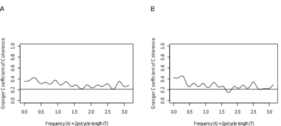
Figure 3, which presents the result of Granger coefficient of coherence
for causality running from GDP (in panel A and B) to electricity consump-tion, shows that at 5% level of significance, GDP Granger-cause electricity consumption at all level of frequencies reflecting long-term, medium-term as
well as short-term business cycles. However, here we observe on difference in
the diagrammatic results reported in panel A and panel B of Figure 3. In panel A we observe a clear evidence that GDP Granger-cause electricity consump-tion and in panel B we find that in the very short range of medium frequencies
(i.e., between 1.6−1.8) we do not find that GDP Granger-causes electricity
con-sumption. Therefore, we found that our interpolation procedure in this case
only has affected the strength as well as evidence of Granger-causality.
Figure 4 presents the result of Granger coefficient of coherence for
62 Tiwari Economia Aplicada, v.18, n.1
A
0.0 0.5 1.0 1.5 2.0 2.5 3.0
0 .0 0 .2 0 .4 0 .6 0 .8 1 .0
Frequency (λ) = 2pi/cycle length (T)
G ra n g e r C o e ff ic ie n t o f C o h e re n c e B
0.0 0.5 1.0 1.5 2.0 2.5 3.0
0 .0 0 .2 0 .4 0 .6 0 .8 1 .0
Frequency (λ) = 2pi/cycle length (T)
G ra n g e r C o e ff ic ie n t o f C o h e re n c e
Figure 3: Granger causality from GDP to electricity consumption. The line parallel to the frequency axis represents the critical value for the null hypothesis, at the 5% level of significance
cycles. In this case too, as with the previous cases, we find that chosen method employed for the interpolation of GDP has little impact on the strength of the Granger-causality.
A
0.0 0.5 1.0 1.5 2.0 2.5 3.0
0 .0 0 .2 0 .4 0 .6 0 .8 1 .0
Frequency (λ) = 2pi/cycle length (T)
G ra n g e r C o e ff ic ie n t o f C o h e re n c e B
0.0 0.5 1.0 1.5 2.0 2.5 3.0
0 .0 0 .2 0 .4 0 .6 0 .8 1 .0
Frequency(λ) =2pi/cycle length (T)
G ra n g e r C o e ff ic ie n t o f C o h e re n c e
Figure 4: Granger causality from electricity consumption to GDP. The line parallel to the frequency axis represents the critical value for the null hypothesis, at the 5% level of significance
4
Conclusions
In the present study we analyzed GC from primary energy consumption and electricity consumption to GDP for the US by using monthly data covering the period of January, 1973 to December, 2009.
consump-The Frequency Domain Causality analysis between Energy Consumption 63
tion (measured either as primary energy or electricity consumption) and real GDP Granger-causes each other at low, intermediate and higher frequencies and thus provide support for the feedback hypothesis. Therefore, energy con-sumption (in general) and real GDP serve as complements to each other. In one hand energy conservation-oriented policies may have a detrimental im-pact of economic growth of the US, on the other to attain higher economic growth path may amplify the energy consumption. Thus, while formulating the policies related to energy and economic growth, the the US government, should keep the bidirectional causal evidence in mind. This is particularly be-cause the feedback relationship between energy consumption and economic
growth increases the effect of energy conservation on economic growth. Say,
for example, when in the first place energy conservation policy is adopted then it will lead to the reduction of economic growth and then low level of economic growth causes the lower level of energy consumption and again eco-nomic growth decreases. Therefore, the US economy should not follow energy
conservation policy for total economy since it causes two opposite effects on
the economy. However, the suggestive point is that the causal relationships between energy consumption and economic growth may be changed at the disaggregated level. Hence, while optimal energy policy may need conserva-tion of energy consumpconserva-tion for some sectors or energy kinds, there may be no need for energy conservation policy for the others and thus optimal portfolio can be obtained in the utilization of various energy sectors or energy kinds.
The unique contribution of the present study lies in decomposing the causality on the basis of time horizons and demonstrating bidirectional short-term, medium-term and long-term causality between the GDP and energy consumption, in general. We have also been able to demonstrate the cyclical nature of the causal relationship between our test variables. Finally, our study has also contributed by showing the strength of the Granger-causality.
Bibliography
Abosedra, S., Dah, A. & Ghosh, S. (2009), ‘Electricity consumption and
eco-nomic growth, the case of lebanon’,Applied Energy86, 429–432.
Acaravici, A. (2010), ‘Structural breaks, electricity consumption and
eco-nomic growth: evidence from turkey’, Journal for Economic Forecasting
2, 140–154.
Aktas, C. & Yilmaz, V. (2008), ‘Causality between electricity consumption
and economic growth in turkey’,ZKÜ Sosyal Bilimler Dergisi4, 45–54.
Altinay, G. & Karagol, E. (2005), ‘Electricity consumption and economic
growth: evidence from turkey’,Energy Economics27, 849–856.
Aqeel, A. & Butt, S. (2001), ‘The relationship between energy consumption
and economic growth in pakistan’, Asia Pacific Development Journal8, 101–
110.
Breitung, J. & Candelon, B. (2006), ‘Testing for short and long-run causality:
A frequency domain approach’,Journal of Econometrics132, 363–378.
Chandran, V. G. R., Sharma, S. & Madhavan, K. (2010), ‘Electricity
64 Tiwari Economia Aplicada, v.18, n.1
Ciarreta, A. & Zarraga, A. (2010), ‘Electricity consumption and economic
growth in spain’,Applied Economics Letters14, 1417–1421.
Diebold, F. X. (2001), Elements of Forecasting, Vol. 2nd Ed., Ohio:
South-Western.
Ghosh, S. (2002), ‘Electricity consumption and economic growth in india’,
Energy Policy30, 125–129.
Granger, C. W. J. (1969), ‘Investigation causal relations by econometric
mod-els and cross-spectral methods’,Econometrica37, 424–438.
Hamilton, J. D. (1994),Time Series Analysis, Princeton University Press.
Ho, C. & Siu, K. (2006), ‘A dynamic equilibrium of electricity consumption
and gdp in hong kong: an empirical investigation’,Energy Policy35, 2507–
2513.
Jamil, F. & Ahmad, E. (2010), ‘The relationship between electricity
consump-tion, electricity prices and gdp in pakistan’,Energy Policy38, 6016–6025.
Jumbe, C. B. L. (2004), ‘Cointegration and causality between electricity
con-sumption and gdp: empirical evidence from malawi’, Energy Economics
26, 61–68.
Kraft, J. & Kraft, A. (1978), ‘On the relationship between energy and gnp’,
Journal of Energy and Development3, 401–403.
Kwiatkowski, D., Phillips, P. C. B., Schmidt, P. & Shin, Y. (1992), ‘Testing the
null hypothesis of stationarity against the alternative of a unit root’,Journal
of Econometrics54, 159–178.
Lean, H. H. & Smyth, R. (2010), ‘Multivariate granger causality between
electricity generation, exports, prices and gdp in malaysia’,Energy35, 3640–
3648.
Lee, C. C. & Chang, C. P. . (2005), ‘Structural breaks, energy consumption,
and economic growth revisited: evidence from taiwan’, Energy Economics
27, 857–872.
Lemmens, A., Croux, C. & Dekimpe, M. G. (2008), ‘Measuring and testing granger causality over the spectrum: an application to european production
expectation surveys’,International Journal of Forecasting24, 414–431.
Lorde, T., Waithe, K. & Francis, B. (2010), ‘The importance of electrical
en-ergy for economic growth in barbados’,Energy Economics32, 1411–1420.
Mozumder, P. & Marathe, A. (2007), ‘Causality relationship between
electric-ity consumption and gdp in bangladesh’,Energy Policy35, 395–402.
Narayan, P. K. & Singh, B. (2007), ‘The electricity consumption and gdp
nexus for the fiji islands’,Energy Economics29, 1141–1150.
Narayan, P. K. & Smyth, R. (2005), ‘Electricity consumption, employment and real income in australia: evidence from multivariate granger causality
The Frequency Domain Causality analysis between Energy Consumption 65
Odhiambo, N. M. (2009a), ‘Electricity consumption and economic growth in
south africa: a trivariate causality test’,Energy Economics31, 635–340.
Odhiambo, N. M. (2009b), ‘Energy consumption and economic growth nexus
in tanzania: an ardl bounds testing approach’,Energy Policy37, 617–622.
Ouédraogo, M. (2010), ‘Electricity consumption and economic growth in
burkina faso: a cointegration analysis’,Energy Economics3, 524–531.
Phillips, P. & Perron, P. (1988), ‘Testing for a unit root in time series
regres-sion’,Biometrica75, 335–346.
Pierce, D. A. (1979), ‘R-squared measures for time series’,Journal of the
Amer-ican Statistical Association74, 901–910.
Priestley, M. B. (1981),Spectral Analysis and Time Series, London Academic
Press.
Shahbaz, M., Tang, C. F. & Shabbir, M. S. (2011), ‘Electricity consumption and economic growth nexus in portugal using cointegration and causality
approaches’,Energy Policy (in press).
Shiu, A. & Lam, L. P. (2004), ‘Electricity consumption and economic growth
in china’,Energy Policy30, 47–54.
Soytas, U., Sari, R. & Ewing, B. T. (2007), ‘Energy consumption, income and
carbon emissions in the united states’,Ecological Economics62, 482–489.
Tang, C. F. (2008), ‘A re-examination of the relationship between
electric-ity consumption and economic growth in malaysia’,Energy Policy36, 3077–
3085.
Tiwari, A. K. (2010), ‘On the dynamics of energy consumption and
employ-ment in public and private sector’, Australian Journal of Basic and Applied
Sciences4(12), 6525–6533.
Tiwari, A. K. (2011a), ‘Energy consumption, co2 emission and economic
growth: a revisit of the evidence from india’, Applied Econometrics and
In-ternational Development11(2), 165–189.
Tiwari, A. K. (2011b), ‘Primary energy consumption, co2 emissions and
eco-nomic growth: Evidence from india’, South East European Journal of
Eco-nomics and Business6(2), 99–117.
Tiwari, A. K. (2012), ‘On the dynamics of energy consumption, co2
emis-sions and economic growth: Evidence from india’, Indian Economic Review
47(1), 57–87.
Yang, H. Y. (2000), ‘A note of the causal relationship between energy and gdp
in taiwan’,Energy Economics22, 309–317.
Yoo, S. H. (2005), ‘Electricity consumption and economic growth: evidence
from korea’,Energy Policy33, 1627–1632.
Yoo, S. H. & Kim, Y. (2006), ‘Electricity generation and economic growth in
66 Tiwari Economia Aplicada, v.18, n.1
Yuan, J., Zhao, C., Yu, S. & Hu, Z. (2007), ‘Electricity consumption and
eco-nomic growth in china: cointegration and co-feature analysis’, Energy
Eco-nomics6, 1179–1191.
Yusaf, M. & Latif, A. (2007), ‘Causality between electricity consumption and economic growth in malaysia: Policy implications’.
URL:http://www.energyseec.com/econometrcis_en.asp
Zachariadis, T. & Pashourtidou, N. (2007), ‘An empirical analysis of
electric-ity consumption in cyprus’,Energy Economics29, 183–198.
Zivot, E. & Andrews, D. (1992), ‘Further evidence on the great crash, the
oil-price shock, and the unit-root hypothesis’,Journal of Business and Economic
The Frequency Domain Causality analysis between Energy Consumption 67
Appendix A
Table A.1: Descriptive statistics
Ln(EC) Ln(PEC) Ln(GDP1) Ln(GDP2)
Mean 5.419443 8.872031 8.995869 9.008425
Median 5.451600 8.877170 8.990502 8.991263
Maximum 5.953059 9.154431 9.498666 9.498123
Minimum 4.877949 8.601188 8.481248 8.487356
Std. Dev. 0.274354 0.131572 0.318821 0.318021
Skewness −0.151128 −0.029806 0.007425 −0.015713
Kurtosis 1.876665 1.970762 1.737696 1.731145
Jarque-Bera (Probability) 24.35831
(0.000005) 19(0.000070).13191 28(0.68538.000001) 28(0.000001).99763
Sum 2341.200 3832.717 3886.215 3891.640
Sum Sq. Dev. 32.44141 7.461121 43.80976 43.59022
Observations 432 432 432 432
4 5 6 7 8 9 10
1975 1980 1985 1990 1995 2000 2005
Ln(EC)
Ln(GDP1) Ln(PEC)Ln(GDP2)