Brazilian Journal of Physics, vol. 37, no. 2B, June, 2007 633
Simple Hadronic Cascade Simulations
Fernando Sep´ulveda and Claudio Dib
Dept. of Physics, Universidad T´ecnica Federico Santa Mar´ıa, Valpara´ıso, Chile
Received on 20 December, 2006
We obtain results for the average number of muons at sea level in a proton-initiated vertical atmospheric cascade using a simple model of hadronic interactions based on the Hillas splitting algorithm. We study the muon yield at sea level as a function of the proton primary energy, varying the parameters of the interaction model in order to see the behavior of our results. We find that our results are in agreement with experimental data and with those of more sophisticated simulation models for some particular values of the model parameters.
Keywords: Hadronic cascade; Hillas splitting; Muon yield
I. INTRODUCTION
The hadronic component of an air shower is the one that continuously feeds the electromagnetic and muonic compo-nents through the decay of neutral and charged mesons re-spectively. The muon yield at detector level is a key signal to determine the energy and composition of the primary cosmic rays [1] and that is the motivation of this study.
In the simulation of hadronic cascades, the most impor-tant ingredient is, of course, the hadronic interaction model, several of which have been developed and are currently used in extensive air shower simulations [2, 3]. We simulate the longitudinal development of proton-initiated vertical cas-cades within a simple hadronic interaction model based on the Hillas splitting algorithm (HSA) which is computationally very fast [4]. According to this model only pions are produced as secondaries; their energies are generated as we explain in section II. Muons, on the other hand, arise from the decay of charged pions. This work is focused on studying the number of muons at sea level as a function of the proton primary en-ergy. Varying the parameters of the interaction model allows us to see the behavior of the muon yield and we can select the values of the parameters for which our results best agree with known ones, either from experiments or other simulations.
In the next section the interaction model is explained and the average multiplicity in single interactions is studied. In sections III and IV we briefly discuss pion decay and the at-mosphere model used. Section V is devoted to the cascade simulation and in section VI results regarding the muon con-tent of the shower are discussed.
II. HADRONIC INTERACTION MODEL
As mentioned above, we study the development of the hadronic component of the shower using a HSA type model for the generation of secondaries in an inelastic hadronic (p-Air orπ±
-Air) interaction. Here the secondaries are all pi-ons and each kind is produced with a probability of one third. Hence, the interactions we consider in the simulations are of the following kind:
p(π±) +Air→p(π±) +Air+X, (1) where X represents any number ofπ±
andπ0.
The energies of the secondaries at each interaction, whether the incoming particle is a proton or a charged pion, are gener-ated by the HSA as follows:
1. Split the available energy of the incoming particle in two parts AandBat random.
2. AssignAas the kinetic energy of the leading particle. This particle is of the same kind as the incoming one.
3. SplitBat random inJ=2Nbranches(Na fixed positive inte-ger).
4. Split one of theJbranches at random in two partsA′andB′.
5. AssignA′as the kinetic energy of a pion.
6. FromB′subtractmπ, split the rest at random in two parts and assign one piece as the kinetic energy of a pion. Call the other pieceB′again.
7. Repeat step 6 until the energy remaining (B′) is less than some preassigned thresholdEth. This value must be at least as large asmπ.
8. OnceEthhas been reached, go back to step 4 with the next branch. Continue until all branches have been used.
This is anenergy priorityalgorithm, which means that en-ergy is conserved at each step, while the multiplicity is aresult of the splitting process.
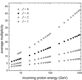
From the description of the algorithm given above, it is clear that the average multiplicity will increase with incoming energy. The algorithm is sensitive to the number of branches J. Tests were run for single interactions withEth=mπ and
J=1,2,4 and 8 in order to see how the average multiplicity varies as a function of the incoming energy. These results are shown in Fig. 1.
634 Fernando Sep´ulveda and Claudio Dib
10 100 1000
0 5 10 15 20 25 30 35 40 45
a
ve
r
a
g
e
m
u
l
t
i
p
l
i
ci
t
y
incoming proton energy (GeV) J = 8
J = 4 J = 2 J = 1
FIG. 1:Average number of secondaries in a p-Air interaction. Each point is the average multiplicity in ten thousand interactions.
growingJ. The valueJ=4 is of special interest because it is suggested as a good interpolation between two more complex hadronic interaction models [3], GEISHA and QGSJET, in the energy region where neither of these models apply: GEISHA is valid for energies below a few tens of GeV and QGSJET is valid above several hundreds of GeV.
III. PION DECAY
The lifetime of the charged pions is of order 10−8s, which makes the decay and interaction processes compete in the de-velopment of the shower. Hence the simulation must include both processes . The decay channels considered are:
π±→µ±+νµ(νµ).
Since the secondary particles are isotropic in the CM, the en-ergies of the products have flat distributions in their kinematic ranges [5]:
m2µ m2
π
·Eπ≤Eµ≤Eπ, (2)
0≤Eν≤Eπ· Ã
1−m 2 µ
m2
π !
. (3)
That is, the muon takes an energy with probability distributed uniformly within the ranges given in equation (2) and the neu-trino carries the rest. These kinematic ranges are valid in the approximation of a highly relativistic pion and massless neu-trinos. In our simulation only muons are tracked down, not the neutrinos.
The lifetime of the neutral pions is of order 10−16s, so even at the highest energies they decay almost instantaneously.
Their decay mode is:
π0→2γ.
Since the photons are isotropic in the CM, their energies have a flat distribution in the range(0,Eπ) for highly relativistic pions.
IV. ISOTHERMAL ATMOSPHERE
Since the natural units for interaction and decay paths are g/cm2 and km respectively, we must have a model for the atmosphere in order to transform among these units. In the simulations we consider an isothermal atmosphere. Within this simple model, the ratio between vertical penetration depth (ing/cm2) and density is constant, this constant represents a height scale and is defined ash0:
h0≡ X
ρ =
X
−dX/dh∝T. (4) In this case, we have an exponential relation between vertical penetration depth and altitude [5]:
X=1030·exp[−h/6.4]g/cm2, (5) withhinkm. This last relation, and its inverse, are used in the simulations to convert the units in pion decay distances from kmtog/cm2.
V. SIMULATION OF THE CASCADES
In this section we discuss in detail the method used for the simulation of the cascades. As was mentioned in section I, we simulate the longitudinal development of vertical cascades initiated by a high energy proton. The processes considered are the following: for protons we only consider inelastic in-teractions with atmospheric nuclei; for charged pions we con-sider interactions and decays; finally, for neutral pions only decays are taken into account. All distances are measured in g/cm2. The basic idea of the algorithm can be summarized as follows:
1. For each particle with energy above the threshold of in-terest and altitude above sea level, determine the dis-tance traveled until a decay or an interaction occurs, de-pending on the case at hand.
2. At that point, generate the corresponding secondaries. Record the depth at which each particle is created along with its energy and kind.
Brazilian Journal of Physics, vol. 37, no. 2B, June, 2007 635
A. Protons in the Cascade
In the case of protons we generate the distance traveled be-tween interactions from an exponential probability distribu-tion using the inversion method. We use an energy-dependent interaction length for protons (in g/cm2) as suggested in ref. [6]:
λp= ½
87 ifE≤0.1TeV
80.8−2.78 ln¡1TeVE ¢ ifE>0.1TeV, (6) whereEis the energy of the incoming proton. Once the inter-action point is known, the secondaries are generated using the HSA as described in section II. When the energy of the proton falls below 10 GeV, no more interactions are considered and the proton is only propagated until it reaches sea level.
B. Charged Pions in the Cascade
In the case of charged pions, we must consider both interac-tion and decay processes. This is done by sampling two dis-tances, one for each process, and selecting theshortestone. If the selected process isinteraction, the secondaries are gen-erated at that point using the HSA as described in section II. Instead, if the selected process isdecay, a muon and a neu-trino are created using a flat distribution as discussed in sec-tion III. For interacsec-tions, the distance traveled is generated in the same way as for protons, but with an interaction length (ing/cm2) [6]:
λπ= ½
116 ifE≤0.1TeV
105−4.23 ln¡ E 1TeV
¢
ifE>0.1TeV, (7) whereEis the energy of the incoming pion. In an isothermal atmosphere, the decay length of charged pions, ing/cm2, is given by [5]:
dπ=EX
επ
, (8)
whereεπ=115GeV,Eis the energy andXis the vertical
pen-etration depth of the pion. Sincedπdepends onX, the distance traveled until decay is not so easily sampled. The natural units for the decay distance are kilometers. Hence, we must gener-ate the decay distance in these units. This is achieved using the inversion method with an exponential probability distribu-tion of mean pathλd=γcτ, whereγandτare the lorentz fac-tor and the mean life of the pion, respectively, together with unit conversion between g/cm2 andkmand viceversa using the exponential relation of equation (5).
The algorithm for the generation of the pion decay distance can be described as follows:
1. Take the initial position of the pionX1, which is in units ofg/cm2, and transform it to a heighth1inkm. 2. Calculateλd=γcτfor the pion in question.
3. Generate the decay distanceldfrom an exponential dis-tribution of mean pathλd.
4. With the decay distance ld, calculate the heighth2at which the pion decays:h2=h1−ld.
5. Transformh2tog/cm2to obtain the final position of the pionX2.
6. The decay distance ing/cm2is thusX2−X1.
The probability for a pion to decay as it traverses a small∆X of atmosphere is∆X/dπ. As can be seen from equation (8),
this probability is negligible ifE≫επ. On the other hand,
decay is the dominating process ifE≪επ. In the simulations
we separate three energy regions for pions:
1. WhenE>1TeVonly interactions are considered. The distance traveled is generated from an exponential prob-ability distribution with mean free pathλπ and secon-daries are generated using the HSA.
2. WhenE <10GeV only decays are considered. The distance traveled until decay is generated as discussed above. The secondaries are created as discussed in sec-tion III.
3. When 10GeV <E <1 TeV, two distances are sam-pled, one for each process just like above, and the process corresponding to the shortest distance is the one that occurs.
C. Neutral Pions in the Cascade
In the case of neutral pions, due to their short lifetime, only decays are considered. The decay is simulated right where the neutral pion is created. The photons produced share the energy of the parentπ0at random, but here we do not treat this part of the process, as it feeds into the electromagnetic component of the shower, which does not subsequently affect the hadronic development.
D. Muons in the Cascade
Muons above threshold are propagated from their point of creation down to sea level without considering any interaction or decay processes. Since we use thresholds above 10 GeV, disregarding decays does not affect the results.
VI. RESULTS AND CONCLUSIONS
636 Fernando Sep´ulveda and Claudio Dib
10 2
10 3
10 4 10
2 10
3 10
4
J = 1 J = 2 J = 4 J = 8 J = 1
J = 2 J = 4 J = 8
a
v.
n
u
m
b
e
r
o
f
m
u
o
n
s
a
t
se
a
l
e
ve
l
primary proton energy (TeV)
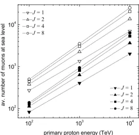
FIG. 2: Average number of muons at sea level as a function of primary energy. Empty and solid symbols correspond to muon energy thresholds of 10 GeV and 30 GeV respectively. Each point is obtained by averaging the muon content in one hundred vertical showers.
Eth[GeV] J C β Eth[GeV] J C β 10 1 10.442 0.7057 30 1 3.3695 0.6943 10 2 10.509 0.7783 30 2 3.4755 0.7548 10 4 9.6191 0.8335 30 4 3.0279 0.8113 10 8 9.8028 0.8528 30 8 2.9945 0.8323
TABLE I:Parameters in the power law for the average number of muons at sea level of equation (9).
Irrespective of the value ofJused, we find that the average number of muons with energies above 10 and 30 GeV at sea level as a function of the primary energy is very well fitted by a power law:
Nµ=C·E0β, (9)
where all correlation coefficients satisfy R2 > 0.999 and 0 < β <1. The values ofβandCdepend on the muon
en-ergy threshold and on the particularJused in the HSA. These values are shown in table I. The general result expressed in equation (9) is expected from what is known from more com-plex models and from experimental results [2, 5].
In table I we can see that for each value ofJthe exponent βis larger for the 10 GeV threshold and grows smoothly asJ goes from 1 to 8. As expected, Fig. 2 shows a marked increase in the number of muons at sea level asJgoes from 1 to 8 for every primary energy. However, each timeJis doubled this increase is progressively slower. For example, take the case of the 10 GeV threshold andE0=100 TeV. WhenJgoes from 1 to 2,Nµ grows in a factor of 1.4; whenJ goes from 2 to 4,Nµgrows in a factor of 1.17; and whenJ goes from 4 to 8, Nµ grows only in a factor of 1.12. This behavior occurs because as the average multiplicity in the HSA grows with J, the average energy per pion decreases, which means the muons produced in the decays are less energetic.
The values ofC andβ for J=4 and 8 are in very good agreement with those obtained by Stanev [2] with the SYBILL model of hadronic interactions [7] and by the simple, deter-ministic model of Matthews [8]. Furthermore, these results are in very good agreement with the experimental results re-ported by the Akeno group [9]. On the other hand; the results obtained withJ=1 and 2 have values forβthat are too low, especially forJ=1. This is due to the extremely low multi-plicity given by the HSA for these values ofJ, as can be seen in Fig. 1.
This simple model for the simulation can be improved in several ways. We can consider a more realistic model for the atmosphere. Also, we can improve on the hadronic interaction model modifying the HSA algorithm by setting the number of branchesJto be energy-dependent and fit hadronic data more precisely.
It is natural to conclude that the parameters in equation (9) are sensitive to the hadronic interaction model. The advantage of this approach lies in the computational speed of the HSA and in its flexibility.
Acknowledgments
This study has been partially funded by Fondecyt, Chile grant no. 1030254.
[1] A. Haungs, H. Rebel, and M. Roth, Rep. Prog. Phys.66, 1145 (2003).
[2] Todor Stanev,High Energy Cosmic Rays, Springer-Praxis 2004. [3] J. Knapp, D. Heck, S.J. Sciutto, M.T. Dova, and M. Risse,
As-tropart. Phys.19, 77 (2003).
[4] A. Hillas, Proc. 17th Int. Cosm. Ray Conf.8, 193 (1981). [5] T. K. Gaisser, Cosmic Rays and Particle Physics, Cambridge
University press 1990.
[6] λis taken as constant for incomingE<0.1TeV, as suggested in ref. [5], and decreasing logarithmically for largerE. This
loga-rithmic term is fitted to the values of Table 5.1 in ref. [5]. These values agree with thep-pandπ-pcollisions listed in S. Eidel-manet al., Phys. Lett. B592, 1 (2004) and converted to p-Air andπ-Air collisions, respectively, according to B. Kopeliovich et al., Phys. Rev. D39, 769 (1989).
[7] R.S. Fletcher, T.K. Gaisser, P. Lipari, and T. Stanev, Phys. Rev. D50, 5710 (1994).