eve asholanda Finite Element Modeling of Flexible Pavements

FINITE ELEMENT MODELING OF FLEXIBLE PAVEMENTS

Áurea Silva de Holanda aurea@det.ufc.br

Federal University of Ceará – Department of Transportation Engineering Campus do Pici, Bl. 703, 60455-760, Fortaleza, Ceará, Brazil

Evandro Parente Junior

Teresa Denyse Pereira de Araújo evandro@ufc.br

denyse@ufc.br

Federal University of Ceará – Department of Structural Engineering Campus do Pici, Bl. 710, 60455-760, Fortaleza, Ceará, Brazil Lucas Tadeu Barroso de Melo

Francisco Evangelista Junior Jorge Barbosa Soares

lucas@det.ufc.br fejr@det.ufc.br jsoares@det.ufc.br

Federal University of Ceará – Department of Transportation Engineering Campus do Pici, Bl. 703, 60455-760, Fortaleza, Ceará, Brazil

Abstract. It is well-known that the analysis of flexible pavements is a difficult task, since

the pavement system is multilayered and three-dimensional. To provide accurate displacements, strains and stresses, the system must consider the different characteristics of each layer. Granular layers, for example, present complex nonlinear stress-strain relationship, while the surface (asphalt) layer displays a time-dependent viscoelastic behavior. Furthermore, cracks and fatigue are some of the problems that the surface layer may present. This paper addresses techniques used in the finite element modeling of flexible pavements. Therefore, appropriate constitutive models and numerical algorithms to represent the nonlinear resilient behavior of the unbound layers and the viscoelastic characteristics of the HMA layer are thoroughly discussed. These techniques are implemented in a computer system developed using an Object-Oriented Programming (OOP) approach. Both axisymmetric and three-dimensional models are included. Several numerical examples will be analyzed in order to validate the implementation and assess the importance of the consideration of the nonlinear and time-dependent effects. The obtained results will be compared with available analytical and computational solutions.

1. INTRODUCTION

The mechanistic or mechanistic-empirical methods have been used in different activities related to the pavement design (Mota, 1991; Medina, 1997; NCHRP/TRB, 2004). It is already known that, in mechanistic methods, the values of stresses and strains calculated in laboratory tests are compared with the ones obtained on-service. The main parameters used for pavement design are tensile stresses/strains at the bottom of the asphalt concrete layer; compressive stresses/strains at the top of the subgrade; and maximum surface deflection. However, the calculation of stresses and strains in pavement structures is a very difficult task because of the complex geometry and boundary conditions inherent to the problem.

It also should be noted that surface and granular layers present a complex constitutive behavior, with nonlinear and time-dependent effects. Thus, a closed-form solution for this type of problem is extremely complicated or even impossible in the practical design situations. These difficulties restrained the use of mechanistic methods in flexible pavement design.

When linear elastic materials are considered, stresses and strains can be calculated using the Multilayer Elastic Theory (Huang, 2004). In this approach, the wheel load is circular and the pavements are considered infinite in horizontal extent. In this way, displacements, stresses and strains are axisymmetric in relation to the center of the load. The superposition principle can be used to determine the influence of all wheel loads because the problem is considered linear.

However, in practice materials are nonlinear, elastic, anisotropic, and inhomogeneous, and some are particulate; viscous and plastic deformations occur in addition to the elastic deformations; loadings are not usually circular or uniformly distributed, and so on (NCHRP/TRB, 2004). Thus, to model pavements correctly, it is necessary to use numerical methods, such as Finite Difference Method, Boundary Element Method and Finite Element Method. The Finite Element Method (FEM) is the most adopted in pavement analysis and will be considered in the following.

The objective of this work is to discuss the main issues involved in the finite element analysis of flexible pavements, such as the nonlinear behavior of the unbound layers, the time-dependent (viscoelastic) behavior of the asphalt layer, and the effect of the distance of the boundaries of the model. This work also presents a finite element system for Computational Analysis of Pavements (CAP3D). This system is currently in active development at the Pavement Mechanics Laboratory of the Federal University of Ceará (LMP/UFC). A set of pavements will be analyzed in order to validate the CAP3D system and to assess the influence of the aspects cited previously.

2. FINITE ELEMENT MODELING

As it was mentioned previously, the calculation of displacements, stresses and strains caused by vehicle loads in pavements is a difficult task even when considering all layers formed by linear elastic materials. In reality, surface and granular layers present a complex constitutive behavior, with nonlinear and time-dependent effects. Such effects should be considered in mechanistic pavement design methodologies, which make use of the pavement structural response into specific distress models (Huang, 2004). Today, there is a trend in the pavement academic community to substitute pavement analysis based on the Multilayer Elastic Theory by analysis based on the Finite Element Method (NCHRP/TRB, 2004).

displacements within each finite element are interpolated using the nodal displacements. On the other hand, the strain vector is obtained from the nodal displacements using appropriate cinematic relations that depend on the problem (e.g plane stress, plane strain, solid). In a matricial form, these relations are:

u B

ε = (1)

where B is the strain-displacement matrix that is independent of the nodal displacements for linear geometrically problems (small strain and displacements). Using the strain vector, stresses (σ) are obtained using the constitutive relation of the material:

) (ε σ

σ= . (2)

Frequently, in the analysis of pavements, the layers are considered homogeneous presenting a linear elastic isotropic behavior. Thus, assuming the linear elastic behavior, Eq. (2) is written as:

ε C σ

σ= 0 + (3)

where σ0 is the vector of initial stresses (e.g. geostatic stresses) and C is the elastic

constitutive matrix that depends not only on the material properties (Young’s Modulus and Poisson’s ratio), but also on the type of the problem, such as plane stress, axisymmetric, and 3D solid (Bathe, 1996).

Using the Virtual Work Principle and considering small strain (as usual for pavement problems), the internal force vector (ge) of a given finite element is given by:

dV dV

W

V t e

V t e

t σ

B g

σ ε g

u =

∫

∫

=δ δ

δ int (4)

that is valid for both linear and nonlinear materials. Considering the existence of proportional loads, the equilibrium equation of the finite element model can be written as:

f u

g

r = ( ) − λ (5)

where is f the external force vector, r is the residual vector and λ is the load factor that controls the load application.

As this equation presents nonlinearities, it is necessary to use appropriate methods to find its solution (Crisfield, 1991). There are some methods used to perform this task, but the most used of them is the Newton-Raphson Method with Load Control. This method is obtained by the linearization of Eq. (5), considering a fixed load level, which yields:

r u

Kδ = − (6)

dV d dV d d _t V t V t B C B K u K σ B

g =

∫

∫

since dσ = C_tdε =C_tB du. In the above equation, Ct is the constitutive tangent matrix.

2.1 Resilient Models

The linear elastic model is extensively used in pavement analysis, mainly due to its simplicity. However, it cannot adequately model the behavior of unbound pavement layers composed by soils and other granular materials (Huang, 2004; NCHRP/TRB, 2004). As a matter of fact, the stress-strain response of a granular soil sample under repeated loading initially presents plastic deformations. It is observed that the amount of plastic flow decreases with cycling until the response is essentially elastic. If the load level is increased above the shakedown level then additional plastic flow occurs, but for lower loads the shaken-down sample exhibits elastic response (Hjelmstad & Taciroglu, 2000). This behavior led the hypothesis that the granular materials composing the unbound pavement layers shake down to a resilient (nonlinear elastic) response under repeated loads.

Due to its simplicity, capacity to fit the response data from cyclic triaxial tests and success in predicting the behavior observed in the field, constitutive equations based on stress dependent “resilient modulus” (Mr) are widely used in the pavement community to model the

sublayers (Huang, 2004; NCHRP/TRB, 2004). The resilient modulus is generally defined as the ratio of the deviatoric stresses (σ1 - σ2) to the axial strain (ε1) in the shakedown regime of

a triaxial test. Several expressions have been proposed to represent the stress dependence of the resilient modulus, as an example, the popular K-θ model assumes that

2

1

k r k

M = θ (8)

where k1 and k2 are parameters obtained fitting the results of cyclic triaxial tests and θ = σx + σy + σz is the first stress invariant. The 2002 Design Guide (NCHRP/TRB, 2004)

recommends the expression

3 2 1 1 k a oct k a a r p p p k M     +    

= θ τ (9)

where pa is the atmospheric pressure (normalizing factor), τoct is the octahedral shear stress

and k1, k2 and k3 are parameters obtained fitting results of cyclic triaxial tests. This expression

can be used to represent the behavior of purely granular (k3 = 0), pure cohesive (k2 = 0) and

mixed soils. In both Eq. (8) and (9) the geotechnical convention that a positive stress means compression should be used.

The constitutive models based on the resilient modulus assume a nonlinear elastic relationship in the form of Eq. (3) with the stress-dependent Mr replacing the conventional

Young’s modulus (E) and considering a constant Poisson’s ratio (v). Since Mr depends on the

final stress state, these models effectively employ a secant C matrix. The stress computation can be easily implemented using this approach, but the same is not true for the computation of the tangent constitutive matrix (Ct) used in the computation of the tangent stiffness matrix,

according to Eq. (7).

matrix can be obtained, but it results in a non-symmetric matrix, which may not be efficient both in terms of memory and computer time. Therefore, the approximate approach resulting in a symmetric tangent matrix suggested in (NCHRP/TRB, 2004) was adopted here.

It is important to note that the Resilient Modulus given by Eq. (8) or (9) are equal to zero for a tension hydrostatic stress state or for a material without pre-compression due to the gravitational stresses. The first problem is solved here prescribing a small Mr (e.g. 0.1 kPa)

whenever the invariant θ is negative. On the other hand, the effect of pre-compression due to the pavement self-weight is considered prescribed a initial stress field where the vertical stresses where (σv) are given by the weight of the superior layers and the horizontal stresses

(σh) depend of the vertical stresses through the relation

v h K σ

σ = 0 (10)

where K0 coefficient of lateral earth pressure at rest. It should be noted that this stress field is

in equilibrium with the initial loads due to self-weight.

2.2 Viscoelasticity

Viscoelastic materials present time and rate-dependent behavior. Thus, their responses do not depend only on the applied load (or displacement) in a specific instant, but of the whole load (or displacement) history (Christensen, 1982). The stress-strain relationship of a viscoelastic material can be given under the form of convolution integrals, which for a uniaxial stress state is written as:

∫

= t

d t

E

0 ( ) τ τ

ε τ

σ . (11)

where E is the relaxation modulus, t is the current time and τ is a time-like parameter starting from the beginning of the loading. The mathematical formulations commonly used in the representation of the viscoelastic behavior of solids are the Prony series

∑

where E_∞, Ei, and ρi are the coefficient of the Prony series and p is the number of terms of this

series. In order to practically compute the convolution integrals a numerical integration scheme should be used (Zocher, 1995; Shen et al., 1995), in which the stress are only computed at prescribed time intervals:

σ σ

σ = + ∆

∆ + = + + n n n

n t t

t

1 1

. (13)

where the subscripts indicates the associated steps, (∆t) is the time step and (∆σ) is the stress increment. Using Eqs. (11) and (12) and assuming a constant strain rate (ε) in each time interval (Zocher, 1995), the stress increment can be written as:

σ ε

σ = ∆ + ∆ ˆ

The first term of the r.h.s. represents the stress increment due to the strain increment (∆ε) between tn and tn+1, with the “tangent” Young’s modulus (E ) given by

∑

i _e i

t E E E 1 / ) 1 ( ρ

ρ _{. (15)}

On the other hand, the term (∆σˆ) represents the stress increment due to the time elapsed since the beginning of the loading process until the current time. This term can be computed from n i p i t S e i

∑

σ (16)

where the parameters S_in can be computed by the recursive expression

1 / 1 / ) 1 ( −∆ − − ∆ − _{+ −}

= t n

i i n i t n i i

i_{S E e}

e

S ρ ρ ρ ε . (17)

In spite of the mathematical complexity of viscoelastic model, its implementation in a finite element is not very difficult. As a matter of fact, for isotropic materials, the computation of the stiffness matrix is rather simple, with the parameter E replacing the conventional Young’s modulus in Eq. (3). On the other hand, the stress computeation is more involved, since it is necessary to store and update a set of variables (e.g., S_in and εn−1) at each Gauss point of a finite element mesh.

3. CAP3D SYSTEM

CAP3D System (Computer Analysis of Pavements) is being developed by the Computer Modeling group of the Pavement Mechanics Laboratory (LMP/UFC) to be used in both pavement design and research. The system is based on the FEM and is implemented in C++ language using Object-Oriented Programming (OOP) techniques (Stroustrup, 1997). The major advantage of adopting this approach is that the program expansion is simpler and more natural, as new implementations have a minimum impact in the existing code. The OOP is particularly useful in the development of large and complex programs, as finite element systems that usually handle different element types, constitutive models and analysis algorithms.

Currently, CAP3D contains both 2D (axisymmetric, plane-strain and plane stress) and 3D analysis models and works with different element shapes (triangular, quadrilateral, bricks, etc.) and interpolation orders (linear and quadratic). It also provides an efficient and accurate modeling of different loading types, including time varying loads. Finally, the system provides different numerical algorithms to nonlinear and time-dependent analysis, as well as a set of constitutive models.

Material, Integration Point, Constitutive Model, and Load. These classes will be briefly discussed in this section.

Figure 1 – The overall class organization.

The Control class provides a common interface for the global algorithms used to analyze a problem. Currently, it is composed of four subclasses: LinearStatic, EquilibriumPath, QuasiStatic and LinearNewmark. The Node class basically stores the nodal data read from the input file (coordinates, support conditions, etc.), as well as some variables computed during the program execution, as the nodal degree of freedom and the current displacements. It also provides a number of methods to query and to update the stored data. The Element class defines the generic behavior of a finite element. The main tasks performed by an object of the Element class are the indication of the number and direction of the active nodal d.o.f., the computation of the element vectors (e.g., internal force) and matrices (e.g., stiffness matrix), and the computation of the element responses (e.g., strains and stresses). The Shape class holds the geometric and field interpolation aspects of the element (dimension, topology, number of nodes, nodal connectivity, and interpolation order).

On the other hand, Analysis Model class handles the aspects related to the differential equation that governs the problem to be solved. It defines the generic behavior of the different models implemented in the program, as the truss, frame, plane stress, plane strain, axisymmetric solid, and 3D solid models. The Integration Point class holds the parametric coordinates and the corresponding weight used for the numerical integration. There are several Integration Point subclasses dealing with different element topologies, as triangles, quadrilaterals, and bricks.

In order to model the material behavior in an efficient way, the system uses two classes: Material and Constitutive Model. Material is a base class that provides a generic interface to handle the data of different materials available in the program, which currently includes the linear elastic, the linear viscoelastic, and the resilient material for the unbound pavement layers. On the other hand, Constitutive Model is a base class that provides a common interface to the different constitutive relations implemented in the program. The main tasks of the Constitutive Model subclasses are the computation of the current stress vector (σ) for a given strain vector (ε) and the evaluation of the tangent constitutive matrix (Ct), to be used in Eq. (7), from the current stress/strain state.

Finally, the Load class was created to allow the generic consideration of natural boundary conditions and body forces. It is a class that provides a common interface for the different loading conditions considered in the program.

4. NUMERICAL EXAMPLES

4.1 Single layer flexible pavement

In order to validate CAP3D implementation, a single layer pavement structure is considered. This structure is composed only by a soft subgrade with Young´s modulus E = 100 MPa and Poisson´s coefficient ν = 0.40. A single wheel load was modeled as a uniform pressure of 550 kPa (p) over a circular area of 150 mm radius (r). The finite element analysis using CAP3D system was performed under linearly elastic axisymmetric conditions. The model used here and depicted in Figure 2 has a horizontal length of 2.1 m (14r) and a depth of 3.0 m (20r) resulting in boundaries at a sufficient distance from the load to represent the unbounded nature of the subgrade. The model was discretized using quadratic quadrilateral elements (Q8).

It should be noted that this example has a simple analytical solution given by Love equation:

( )

[

]

   

  

+ − =

2 3 2

1 1 1

z r p

v

σ (18)

where σv represents the vertical stresses in a given depth (z). The finite element results are

presented in Table 1 and compared with Love´s solution. It can be noted that a very good agreement was obtained in all cases.

Figure 2 - Finite element mesh.

Table 1. Comparison of vertical stresses (kPa).

Depth(mm) Analytical result CAP3D Error (%)

0.00 -550.00 -550.85 0.15

100.00 -456.13 -457.70 0.34

4.2 Three-layer pavement analysis

The stress in the natural subgrade computed in the previous example is very high. Therefore, two layers (asphalt surface and base) composed of more stiff and resistant materials will be used between the wheel load and the natural soil. These layers distribute the load in a larger area resulting in small stresses at the top of the subgrade. The pavement structure considered here consists of 100 mm of asphalt concrete (E = 3500 MPa e ν = 0.35) over 200 mm of crushed stone base (E = 350 MPa e ν = 0.30) over the same soft subgrade (E = 100 MPa e ν = 0.40) considered previously.

The analysis using CAP3D system was performed under linearly elastic axisymmetric conditions. A single wheel load was modeled as a uniform pressure of 550 kPa over a circular area of 150 mm radius. The same discretization of the previous example was used here. Vertical and horizontal stresses were computed in different depths of the pavement structure and the results were compared with the ones obtained using Everstress and MICHPAVE systems, mentioned previously.

Table 2 presents the results of vertical stresses (kPa) and it can be observed that they are very similar to the ones obtained using Everstress e MICHPAVE. It also should be noted that this agreement is even better with Everstress system. Probably, this difference is caused by the limitation of MICHPAVE system related to the mesh refinement. Moreover, MICHPAVE only uses quadrilateral linear elements. It is very interesting to compare the vertical stresses in the top of the natural subgrade (63.35 kPa) with the pressure applied at the top of the asphalt layer (550 kPa). These results show that the one of the most important functions of the pavement layers is to distribute the stress on a large area reducing the stresses that reach the natural soil which generally has a lower resistance.

Table 2. Comparison of vertical stresses (kPa).

Depth(mm) CAP3D Everstress MICHPAVE 0.00 -555.34 -550.00 -550.00 99.99 -244.31 -247.96 -277.29 100.01 -248.10 -247.93 -277.29 299.99 -63.35 -63.58 -61.57 300.01 -61.41 -63.58 -61.57

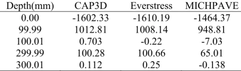
Table 3 presents the results for horizontal stresses computed by CAP3D, Everstress and MICHPAVE. Once again, the results computed by the proposed system are in better agreement to the ones obtained by Everstress system.

Table 3. Comparison of horizontal stresses (kPa).

Depth(mm) CAP3D Everstress MICHPAVE 0.00 -1602.33 -1610.19 -1464.37 99.99 1012.81 1008.14 948.81 100.01 0.703 -0.22 -7.03 299.99 100.28 100.66 65.01 300.01 0.112 0.25 -0.138

However, as this implementation is not finished yet, the subgrade was modeled using conventional finite elements based on the recommendation that the horizontal lower boundary of the finite element mesh be located no closer than 18 tire radii for a homogeneous elastic system and no closer than 50 tire radii for a layered system (NCHRP/TRB, 2004). It is also recommended that the vertical side boundary of the finite element mesh be located at least 12 tire radii from the center of the tire.

Table 4 illustrates the results obtained using these recommendations and it can be noticed that the results are in very good agreement with the ones calculated by Everstress and MICHPAVE. As it occurred with the stresses, the displacements are closer to the ones obtained by Everstress system.

Table 4. Displacements (mm).

Depth(mm) CAP3D Everstress MICHPAVE 0.00 0.439 0.448 0.471 99.99 0.433 0.442 0.465 100.01 0.433 0.442 0.465 299.99 0.341 0.350 0.376 300.01 0.341 0.350 0.376

4.3 Pavement with nonlinear behavior

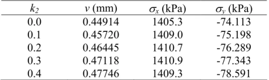
In this example the influence of the nonlinear behavior of the granular base is taken into account using the Resilient Model described by Eq. (9). The geometry, loading, boundary conditions, mesh discretization, and material properties of asphalt and subgrade layers are the same ones used in Example 4.2, but the parameters used here to describe the behavior of the base layer are pa = 100 kPa, k1 = 2000.0, k3 = 0.0. A variable k2 was considered here since the

aim of this example is to assess the influence of the nonlinear effects both pavement response and performance of the numerical algorithm used for nonlinear analysis.

Table 5. Results of the nonlinear pavement analysis.

k2 v (mm) σx (kPa) σy (kPa)

0.0 0.44914 1405.3 -74.113

0.1 0.45720 1409.0 -75.198

0.2 0.46445 1410.7 -76.289

0.3 0.47118 1410.9 -77.343

0.4 0.47746 1409.3 -78.591

The displacements at the surface (v), the horizontal tensile stresses at the bottom of the asphalt layer (σx) and the vertical compressive stresses at the top of the subgrade (σy)

computed by the CAP3D system are presented in Table 5. It shows that the consideration of the nonlinear effects leads to greater displacements and vertical stresses. This effect increases with the value of the k2 parameter.

The increase of the k2 parameter has also a serious impact on the convergence of the

Newton-Raphson algorithm used to carry-out the nonlinear analysis of the model. The net effect of an increase of this parameter is an increase in the nonlinearity of the stress-strain behavior, which increases the required number of iterations required to achieve convergence. As a matter of fact, convergence was not achieved here for k2 greater than 0.4, probably due

the 2002 Design Guide (NCHRP/TRB, 2004). Therefore, further studies are necessary to solve this problem in a more satisfactory way.

4.4 Viscoelastic flexible pavement analysis

The geometry, loading, boundary conditions, mesh discretization, and material properties of asphalt and subgrade layers of this example are the same ones used in Example 4.2. However, in order to evaluate the effects of the viscoelastic behavior of the asphalt layer in the mechanical response of the pavement the relaxation modulus is given behavior of the asphalt layer is described by the Prony series presented in Table 7. The Prony series coefficients were extracted from Lee (1996) for the creep compliance shown in Figure 5. This asphalt mixture is a HMA fabricated under SHRP (1994) specifications.

Table 7. Prony series of the asphalt layer.

i Ei (kPa) ρi

∞ 1.172E+06 -

1 3.10E+09 2.20E-05

2 4.31E+09 2.20E-04

3 3.46E+09 2.20E-03

4 2.02E+09 2.20E-02

5 1.27E+09 2.20E-01

6 2.72E+08 2.20E+00

7 6.59E+07 2.20E+01

8 1.45E+07 2.20E+02

9 1.52E+06 2.20E+03

10 7.10E+05 2.20E+04

11 5.88E+04 2.20E+05

When the time-dependent viscoelastic effects are included the duration and time variation of the applied load are of great importance. Therefore, it is important to relate vehicle speed with the loading time. According to Brown (1973) the relation between loading time t (s), depth beneath the pavement surface d (m), and vehicle speed v (km/h), is given by:

log t = 0.5d - 0.2(1 - 4.7 log v) (19)

The loading time as defined by this equation is equal to the inverse of the angular frequency of the applied sinusoidal wave. In order to investigate the effect of the viscoelastic behavior under vehicle speed over the asphaltic surface layer, 3 sine half-wave pulses of 0.01 s, 0.015 s and 0.1 s equivalent to speeds of 100 km/h, 60 km/h and 10 km/h, were calculated by Eq. (19). The displacements at the surface (v), the horizontal tensile stresses at the bottom of the asphalt layer (σx) and the vertical compressive stresses at the top of the subgrade (σy)

computed by the CAP3D system are presented in Table 5.

Table 8. Results of the elastic and viscoelastic models.

Behavior Pulse (s) v (mm) σx (kPa) σy (kPa)

Viscoelastic 0.010 0.4184 1263.0 -57.400 Viscoelastic 0.015 0.4278 1164.3 -59.217 Viscoelastic 0.100 0.4743 714.29 -66.703

Elastic All 0.4637 765.80 -66.003

The obtained results show that with respect to the displacements at the asphalt layer, the difference between the two considerations (elastic and viscoelastic) is more relevant when longer pulse durations are applied. As the equivalent elastic Young´s Modulus was determined at the 0.1 s pulse, the differences between the viscoelastic and elastic response for this time duration are small, except of the tensile horizontal stresses. However, the differences are significant for the other pulses. Decreasing differences are observed when pulse duration increases (until 0.1 s pulse). For these cases the viscoelastic calculated displacements are smaller than the elastic ones. Similar behavior is observed for vertical stresses (σyy) at the top of subgrade. On the other hand, large differences occur for the tensile stress at the bottom of the asphalt layer for all analyzed cases.

5. CONCLUSIONS

This paper discussed some important aspects of the finite element analysis of flexible pavements, as the nonlinear resilient behavior of the granular layers and the time-dependent (viscoelastic) behavior of the asphalt. The theoretical aspects of these constitutive models were discussed and the finite element system (CAP3D) implementing these models was described.

This computational system was validated using analytical solution and computer results obtained by other pavement programs for pavement analysis. It was also verified that the position of the boundaries of the model has a greater influence over the displacements than over the stresses. This problem was solved using more distant boundaries and a course mesh in this region. With that a very good agreement was obtained for the available solutions.

The influence of the stress-dependent resilient modulus of the granular layers was also studied. The numerical example considered here, showed that the consideration of the nonlinear behavior affects the displacements at the top asphalt layer and the stresses at the top of the subgrade, both of them are important parameters in the mechanistic design of pavements.

The time-dependent analysis demonstrated that the use of the conventional Young´s Modulus based on the standard 0.1s pulse leads to acceptable results for the displacements at the top asphalt layer and vertical stresses at the top of the subgrade for this loading pulse. On the other hand, it leads to very poor results for the tensile horizontal stresses at the bottom of the asphalt layer, not only for this pulse but also for all the other loading pulses.

Acknowledgements

The authors would like to acknowledge the financial support of FINEP/CTPETRO (Cooperative Project 03 – Analysis of Asphalt Pavements).

REFERENCES

ASTM (1982). ASTM D 4123 - Standard Method of Indirect Tension Test for Resilient Modulus of Bituminous Mixtures. American Society of Testing and Materials.

Bathe, K. J., 1996. Finite Element Procedures. Prentice-Hall

Brown, S. F. (1973). Determination of Young’s modulus for bituminous materials in pavement design. Highway Research Record, 431:38–49.

Christensen, R. M., 1982. Theory of Viscoelasticity. Dover, New Nork, NY, USA, 2nd edition.

Cook, R., Malkus, D., Plesha, M., 2002. Concepts and Applications of Finite Element Analysis. 2a Edição, Editora John Wiley & Sons.

Crisfield, M. A., 1991. Non-linear Finite Element Analysis of Solids and Structures, 1, John Wiley and Sons.

DNER (1994). DNER-ME 133/94: Determinação do Módulo de Resiliência de Misturas Betuminosas. Departamento Nacional de Estradas de Rodagem, Brazil. in Portuguese. Harichandran, R.S., Yeh, M.-S., and Baladi, G.Y., 1990. “MICHPAVE: A Nonlinear Finite

Element Program for the Analysis of Flexible Pavements,” Transportation Research Record, 1286.

Hjelmstad, K. D., Taciroglu, E, 2000. Analysis and Inplementation of Resilient Modulus Models for Granular, Journal of Engineering Mechanics - ASCE, 126(8), pp. 821-830.

Huang, Y. H., 2004. Pavement Analysis and Design. Prentice Hall, Inc., Englewood Cliffs.

Lee, H. J. (1996). Uniaxial Constitutive Modeling of Asphalt Concrete Using Viscoelasticity and Continuum Damage Modeling. PhD thesis, Civil Engineering Department, North Caroline University, North Caroline, NC, USA.

Martha, L. F. and Parente Jr, E., 2002. An Object-Oriented Framework for Finite Element Element Programming, WCCM, Vienna, Austria.

Medina, J. ,1997. Mecânica dos Pavimentos, 1 ed. COPPE/UFRJ., 380 p.

NCHRP/TRB, 2004. Guide for Mechanistic-Empirical Design of New and Rehabilitated Pavement Structures, Appendix RR: Finite Element Procedures for Flexible Pavement Analysis.

SHRP (1994). SHRP-A-415: Permanent Deformation Response of Asphalt Aggregate Mixes. Strategic Highway Research Program, Washington, D.C., USA.

Stroustrup, B., 1997. The C++ Programming Language, Third edition, Addison-Wesley.