ISSN 0104-530X (Print) ISSN 1806-9649 (Online)
Resumo: A Programação por Metas (Goal Programming - GP) é uma abordagem multicritério da Pesquisa Operacional que vem sendo empregada na solução de complexos problemas de decisão. Este trabalho propõe um novo modelo de Programação por Metas Fuzzy (Fuzzy Goal Programming - FGP) para tratar o processo de orçamento de capital de empresas em um ambiente econômico sob incerteza. Para fins de comparação de desempenho, o modelo FGP e outro modelo desenvolvido com os mesmos fins, recentemente publicado, foram aplicados considerando-se os dados de uma empresa que foi o objeto do estudo. A modelagem e otimização foram feitas com o software GAMS - 23.6.5 e utilizando-se o solver CPLEX. Os resultados do modelo FGP proporcionaram melhorias com relação aos obtidos com o modelo alternativo citado, por exemplo: aumento do índice de lucratividade, redução do payback e melhor aplicação do capital disponível no orçamento. Além disto, o modelo FGP tem características de flexibilidade que permitem ao gestor simular, obter resultados rapidamente e com facilidade, acerca de cenários sob incerteza de seu interesse.
Palavras-chave: Programação por Metas Fuzzy; Orçamento de capital; Ambiente econômico sob incerteza. Abstract: The Goal Programming (GP) is a multi-criteria approach of Operational Research that has been used for solving complex decision problems. This paper proposes a new Fuzzy Goal Programming (FGP) model to handle the process of capital budget of companies in an economic environment under uncertainty. For performance comparison purposes, the FGP and another recently published model developed for the same purposes were applied to data from a company that was the object of the study. The modeling and optimization were made with the GAMS software - 23.6.5 and using the CPLEX solver. The results obtained from the FGP model provided higher improvements than those obtained with the alternative model, as for example: increased profitability index, reduced payback and better application of the capital available in the budget. Furthermore, the FGP model has flexibility features that allow the manager to simulate, quickly and easily obtaining results about scenarios under uncertainty. Keywords: Fuzzy Goal Programming; Capital budget; Economic environment under uncertainty.
Fuzzy Goal Programming applied to the process of
capital budget in an economic environment under
uncertainty
Programação por Metas Fuzzy aplicada ao processo de orçamento de capital em um ambiente econômico sob incerteza
Aneirson Francisco da Silva1
Fernando Augusto Silva Marins1
Erica Ximenes Dias1
Rafael de Carvalho Miranda2
1 Faculdade de Engenharia, Universidade Estadual Paulista – UNESP, Av. Ariberto Pereira da Cunha, 333, CEP 12516-410, Guaratinguetá, SP, Brazil, e-mail: [email protected]; [email protected]; [email protected]
2 Universidade Federal de Itajubá – UNIFEI, Campus Prof. José Rodrigues Seabra - Sede, Av. BPS, 1303, Bairro Pinheirinho, Caixa Postal 50, CEP 37500 903, Itajubá, MG, Brazil, e-mail: [email protected]
Received June 1, 2015 - Accepted Oct. 26, 2015
Financial support: This research was partially supported by The National Council for Scientific and Technological Development (CNPq - 306214/2015-6, CNPq - 431758/2016-6), São Paulo Research Foundation (FAPESP - 2015/12711-4; FAPESP - 2015/24560-0), and FAPEMIG (APQ-01188-16).
1 Introduction
In complex industrial problems, the decision taking involves inaccurate or incomplete information, multiple decision agents and, in general, multiple
objectives that can be conflicting with each other (Deb, 2001). This is the case of investment project
• Net Present Value Method (NPV) – it allows comparing initial investments with future returns, in which, when the NPV is positive, it means that the capital invested will be recovered;
• Internal Rate of Return Method (IRR) – it considers
the discount rate that equates the inflows and outflows of an investment, in which, for the
project to be viable, the value of the IRR must be greater than or equal to the Minimum Attractive Rate of Return (MARR) adopted by the company;
• Payback Method – it analyzes the recovery period of the invested capital, that is, the period necessary to a certain investment can be paid;
• Profitability Index Method (PI) – it considers
the ratio between the NPV of net cash inflows
of the project and the initial investment value.
In this type of problem, the budget constraint plays important role with respect to limit the decisions that can be taken in the selection of the investment projects, and it is recommended the use of optimization techniques aiming at the optimal allocation of available
financial resources (Abensur, 2012).
In this sense, an alternative is to apply to this type of complex and critical situation for companies, the models and techniques of the Goal Programming (GP). In fact, the GP is a method of Operational Research (OR), which allows the modelling and solution of multiobjective problems, including under the occurrence of uncertainties, as is typical in economic scenarios associated with decisions in investment portfolios (Silva & Marins, 2014). Some researchers developed interesting related works:
• Bradi et al. (2000) applied a binary GP model to the problem of project selection, without considering the occurrence of uncertainty;
• Lee & Kim (2000) combined the ANP (Analytic Network Process) (Saaty, 2006) with the GP to select information system projects;
• Santos et al. (2012) investigated the performance of business managers based on the knowledge about cost management and budget participation;
• Ghahtarani & Najafi (2013) combined the robust stochastic optimization (Mulvey et al., 1995) with the GP, developing the Robust Goal Programming (RGP) model, which was applied in selecting investment portfolios in the stock market;
• Bakirli et al. (2013) combined the AHP method (Saaty, 1977) and a Fuzzy Goal Programming
(FGP) model with the QFD (Quality Function Deployment) matrix (Lam & Lai, 2015), to select projects that offer the maximum benefits when
performed within various budgets;
• Abensur (2013) evaluated the capital budget in a context in which the managers can establish the completion sequence of projects previously selected, which minimizes the need for investment;
• Khalili-Damghani et al. (2013) applied the FGP model combined with the TOPSIS - Technique for Order Preference by Similarity to Ideal Solution multicriteria method (Joshi & Kumar, 2016) to select multi-period projects in a context under uncertainty;
• Li & Wan (2014) developed a Fuzzy Linear Programming model for the selection of supply chain projects.
Although there are many studies linked to the selection of investment projects, the use of Fuzzy Goal Programming (FGP) models in this type of problem is recent, corroborating therefore the importance of this research. So, this study aimed to develop and apply a FGP model to solve the capital budget problem. In addition, it was performed a comparison of its results with those obtained by Abensur (2012), who proposed, recently, an alternative model to the same class of investment problems.
Considering the classification proposed by Bertrand & Fransoo (2002), this research can be classified as an
applied research, because it provides contributions for the current literature, possessing normative empirical objective, since the model aims to understand policies and strategies that allow actions to better understand a current situation. Besides, with respect to the form of approach of the problem, the research is quantitative type and the research method adopted is the modeling.
This article is organized in 5 sections. Section 2 briefly
describes the theoretical foundations of the GP and, in particular, addresses the FGP model. Section 3 addresses the problem description; Section 4 presents the problem
modeling and the results obtained; finally, Section 5
brings the conclusion and the recommendations for future researches, followed by the bibliography.
2 Goal programming
• Weighted Goal Programming (WGP) – weights are attributed to the (positive and negative) deviation variables with regard to the goals
chosen for the objectives. This was the first
model of GP developed and, due to this; it will
be briefly described below;
• Lexicographic Goal Programming (LGP) or Preemptive Goal Programming – objective functions are ordered according to their importance established from a prioritization made by the managers;
• Minmax Goal Programming (Minmax GP) – objective functions, which consider the sum of the deviation variables, are included in the model.
2.1 Weighted Goal Programming
In the WGP models, the deviation variables present equivalent hierarchies, being the weighting what will distinguish the most important objectives. The decision-makers need to estimate the weights in
such a way that a large part of the objectives is satisfied,
which generates problems with the subjectivism in the estimation of these weights. To try minimizing the subjectivism, a method that has been very adopted in the prioritization of objectives is the Analytic Hierarchy Process – AHP (Saaty, 1977).
According to Martel & Aouni (1998), the original WGP model can be expressed by:
Equation 1 βe α are weights attributed, respectively, to d and di i
+ −
1
( )
n
i i i i i
Min βd+ αd−
= +
∑
(1)Subject to:
Constraint 2 where x is the vector of the decision variables of the model xi; fi (x) is an objective function
I, gi is a goal value chosen to fi, d and di+ i− are,
respectively, the auxiliary (positive and negative) deviation variables related to the goal gi
( ) , 1, 2,..., .
i i i i
f x d− ++d−=g i= n (2)
Constraint 3 A and c are, respectively, a matrix of
the LHS (Left Hand-Side) coefficients and a RHS
(Right Hand-Side) vector for hard restrictions in the original multi-criteria model, and F is Feasible set.
Ax ≤ c (3)
Constraint 4 It is observed that, by only one of the deviation variable associated with each goal can have value different from zero.
, , 0, . 0, 1, 2,..., .
i i i i i
x d+ d− ≥ d d+ −= i= n x∈F (4)
There are other deterministic GP models; however, they are not presented in this work, for more details it is recommended to consult a GP review by Silva & Marins (2015).
2.2 Fuzzy Goal Programming (FGP) Model
It should be noted that management decision problems have as natural characteristics the occurrence of uncertainty in their parameters, such as, for example, problems related to aggregate production planning and budgetary problems (Wang & Liang, 2004). The main GP models under uncertainty are (Silva & Marins, 2015):
- Multi-Choice Goal Programming (Chang, 2007);
- Revised Multi-Choice Goal Programming (Chang, 2008);
- Integer Multi-Choice Goal Programming (Silva et al., 2013a);
- Fuzzy Multi-Choice Goal Programming (Bankian-Tabrizi et al., 2012);
- Multi-Segment Goal Programming (Liao, 2009);
- Revised Multi-Segment Goal Programming - RMSGP (Chang et al., 2012a);
- Multi-Coefficients Goal Programming - MCGP
(Chang et al., 2012b);
- Revised multi-choice Goal Programming - LHS (Silva et al., 2015);
- Fuzzy Goal Programming - FGP (Silva & Marins, 2014; Jamalnia & Soukhakian, 2009; Yaghoobi & Tamiz, 2007; Liang & Wang, 1993; Zimmermann, 1978);
- Robust stochastic optimization (Mulvey et al., 1995).
In this research, it was applied the FGP model, because it is the oldest GP model under uncertainty, having a wide range of real applications (Silva & Marins, 2014, 2015). Concepts and results relating to the inclusion of uncertainty occurrence in the problem data, the contribution of the GP, and the basic theory of Fuzzy sets to handle these situations are presented (Chang, 2007).
Zimmermann (1978) used the triangular fuzzy number to characterize linguistic values and Liang
& Wang (1993) justified the use of triangular fuzzy
This was the option adopted in this work that is going to be detailed subsequently.
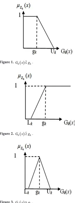
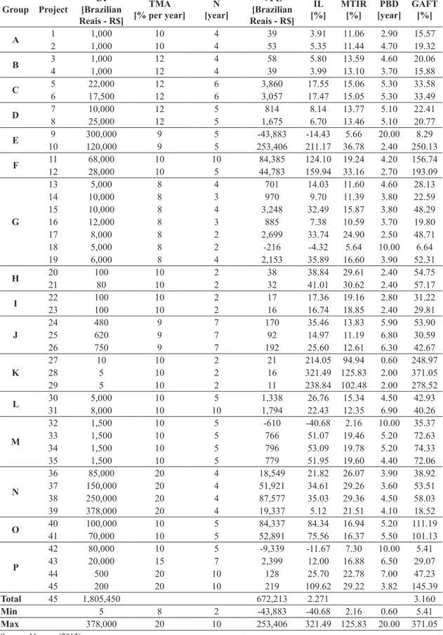
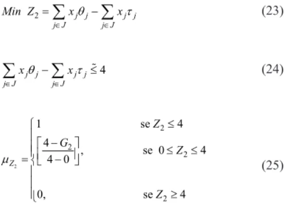
In this line, according to Jamalnia & Soukhakian (2009), and Yaghoobi & Tamiz (2007), there are three most common types of pertinence functions, denoted by µZk for a given objective function Gk, when we
are working with triangular fuzzy numbers, as show the expressions (5)-(7) and illustrate the Figures 1-3. It was adopted the notation [~] to represent a fuzzy goal value (desired and imprecise) gk chosen to a fuzzy objective function Gk:
Equation 5 there is a fuzzy objective function of the type “the lower its value in relation to gk, the better it is”;
( ) , 1,... ,
Gk x ≤gk k= m (5)
Equation 6 there is a fuzzy objective function of the type “the higher its value in relation to gk, the better it is”
( ) , 1,..., ,
k k
G x ≥g k= +m n (6)
Equation 7 there is a objective function that is wanted to be achieved exactly at the value gk chosen.
( ) , 1,..., .
k k
G x ≅g k= +n l (7)
The fuzzy goals can be identified as fuzzy sets defined on the feasible set of solutions associated with
a pertinence function. The linear pertinence functions are the functions most adopted both in the theoretical and practical works (Jamalnia & Soukhakian, 2009). For the fuzzy constraints (5) and (6), by adopting the triangular fuzzy numbers, in which Lk and Uk, respectively, are the minimum and maximum values chosen by the decision-maker to be attributed to the fuzzy goal gk, the linear pertinence functions can be expressed by (8)-(10):
1 se ( ) ( )
( ) se 1,....,
0 se
k
k k
k k
Z k k k
k k
k k
G x g
U G x
x g G (x) U k m
U g
G (x) U µ
≤
−
= − ≤ ≤ =
≥
(8)
1 se ( ) ( )
( ) se 1,....,
0 se
k
k k
k k
Z k k k
k k
k k
G x g
G x L
x L G (x) g k m n
g L
G (x) L
µ
≥
−
= − ≤ ≤ = +
≤
(9)
0 ( )
se ( )
( ) 1,...,
( ) se
0 se
k
k k
k k k
k k Z
k k
k k k
k k
k k
U G x
L G x g
U g
x k n l
U G x
g G (x) U
U g
G (x) U
µ −
≤ ≤
−
= − = +
≤ ≤
−
≥
(10)
Other form to visualize this pertinence functions is in Figures 1-3:
It is observed that, usually, the limits Lk and Uk are subjectively chosen by the decision-makers, or are associated with the tolerances existing in a technical process. The choice of these tolerance limits is very
important, once they directly influence the model
optimization (Silva & Marins, 2014).
The model of the Fuzzy Goal Programming (FGP), proposed by Yaghoobi & Tamiz (2007), using the triangular pertinence functions, can be expressed by:
Equation 11 objective function aims to maximize the
total degree of fuzzy achievement and, when λ =1, it means that all fuzzy goals were fully satisfied or met.
Max λ (11)
Figure 2.Gk( )x ≥gk.
Figure 1. ( )
k k
G x ≤g .
Subject to:
Constraint 12 represents a situation for which it is desired to penalize the positive deviation.
( ) , 1, 2,...,0
i i i
G X −d+≤g i= i (12)
Constraint 13 represents a situation for which it is desired to penalize the negative deviation.
( ) , 0 1, 2,..., 0
i i i
G X +d−≥g i i= + j (13)
Constraint 14 represents a situation for which it is desired to penalize both positive and negative deviations.
( ) , 0 1, 2,...,
i i i i
G X +d−−d+=g i j= + K (14)
Constraints 15 to 17 are related to the limitations imposed to the degree of achievement of the scenarios associated to constraints (5)-(7).
0
1
1 , 1, 2,...,
i iU
d i i
λ+ +≤ =
∆ (15)
0 0
1
1, 1, 2,...,
i iL
d i i j
λ+ −≤ = +
∆ (16)
0
1 1
1, 1,2,...,K
i i
iL iU
d d i j
λ+ −+ +≤ = +
∆ ∆ (17)
Constraints 18 to 19 indicate the domains of variables.
. 0, 1, 2,..., i i
d d+ −= i= K (18)
,di,di 0,
λ + −≥
X∈F (F is a feasible set) (19)
where λ = i i
λ
∑
is the degree of achievement of the fuzzy goals, gi is the level of aspiration (or desired value) for the objective function Gi, ∆iLand∆iUare, respectively, the difference between the minimum value (L) and the maximum value (U) with respect to the goal gi.It can be observed that λ ∈i [ ]0,1 and, when the value of λi=1, it means that the fuzzy, goal gi was
fully achieved. In this
In the sequence, it is presented the capital budget problem and the steps followed for its resolution.
3 Problem description and research
steps
In this article, the FGP model was applied to the capital budget problem, considering the economic environment in which there is occurrence of uncertainties in the data and parameters involved in the decision taking. The research steps were:
• Problem identification – It was chosen the capital budget problem proposed and studied by Abensur (2012), in which it is desired to select, among a set of 45 investment projects, which projects should be executed;
• Data collection – The data used were those available in Abensur (2012) and they are in Table 1;
• Modeling, model solution and comparison of results – The FGP model was developed and implemented using the GAMS software - version 23.6.5, and was solved using the CPLEX Solver, as described in Section 4 (GAMS, 2014).
For the comparison between the results of the FGP model and the model of Abensur (2012), three objective functions were considered, related to:
• The Profitability Index (PI) – given by the ratio between the NPV and the initial payout value;
• The Total Discounted Payback (TDP) – associated with the time taken to recover the capital invested;
• The Degree of Total Financial Leverage (DTFL) – is a risk measure to evaluate investment projects.
The constraints considered in the model by Abensur (2012) are relating to:
• Mutually exclusive relationships and relationships of dependence of projects;
• Investment limits foreseen for the projects;
• Additional relationships that ensure that the
projects of the optimal solution have Modified
Internal Rate of Return (MIRR) above the Minimum Acceptable Rate of Return (MARR),
PI above 1 and TDP lower or equal to the useful
life (economic life or their duration) of projects. The model by Abensur (2012) also has as premises that:
• All projects begin their activities on the same initial date;
• The project groups are independent of each other;
• There are groups with mutually exclusive projects;
• There are independent projects;
• There are projects with relationship of dependence;
Table 1. Projects analyzed and their respective indicators of profitability, risk and return.
Group Project
DI [Brazilian Reais - R$]
TMA [% per year]
N [year]
VPL [Brazilian Reais - R$]
IL [%]
MTIR [%]
PBD [year]
GAFT [%]
A 1 1,000 10 4 39 3.91 11.06 2.90 15.57
2 1,000 10 4 53 5.35 11.44 4.70 19.32
B 3 1,000 12 4 58 5.80 13.59 4.60 20.06
4 1,000 12 4 39 3.99 13.10 3.70 15.88
C 5 22,000 12 6 3,860 17.55 15.06 5.30 33.58
6 17,500 12 6 3,057 17.47 15.05 5.30 33.49
D 7 10,000 12 5 814 8.14 13.77 5.10 22.41
8 25,000 12 5 1,675 6.70 13.46 5.10 20.77
E 9 300,000 9 5 -43,883 -14.43 5.66 20.00 8.29
10 120,000 9 5 253,406 211.17 36.78 2.40 250.13
F 11 68,000 10 10 84,385 124.10 19.24 4.20 156.74
12 28,000 10 5 44,783 159.94 33.16 2.70 193.09
G
13 5,000 8 4 701 14.03 11.60 4.60 28.13
14 10,000 8 3 970 9.70 11.39 3.80 22.59
15 10,000 8 4 3,248 32.49 15.87 3.80 48.29
16 12,000 8 3 885 7.38 10.59 3.70 19.80
17 8,000 8 2 2,699 33.74 24.90 2.50 48.71
18 5,000 8 2 -216 -4.32 5.64 10.00 6.64
19 6,000 8 4 2,153 35.89 16.60 3.90 52.31
H 20 100 10 2 38 38.84 29.61 2.40 54.75
21 80 10 2 32 41.01 30.62 2.40 57.17
I 22 100 10 2 17 17.36 19.16 2.80 31.22
23 100 10 2 16 16.74 18.85 2.40 29.81
J
24 480 9 7 170 35.46 13.83 5.90 53.90
25 620 9 7 92 14.97 11.19 6.80 30.59
26 750 9 7 192 25.60 12.61 6.30 42.67
K
27 10 10 2 21 214.05 94.94 0.60 248.97
28 5 10 2 16 321.49 125.83 2.00 371.05
29 5 10 2 11 238.84 102.48 2.00 278.52
L 30 5,000 10 5 1,338 26.76 15.34 4.50 42.93
31 8,000 10 10 1,794 22.43 12.35 6.90 40.26
M
32 1,500 10 5 -610 -40.68 2.16 10.00 35.37
33 1,500 10 5 766 51.07 19.46 5.20 72.63
34 1,500 10 5 796 53.09 19.78 5.20 74.33
35 1,500 10 5 779 51.95 19.60 4.40 72.06
N
36 85,000 20 4 18,549 21.82 26.07 3.90 38.92
37 150,000 20 4 51,921 34.61 29.26 3.60 53.51
38 250,000 20 4 87,577 35.03 29.36 4.50 58.03
39 378,000 20 4 19,337 5.12 21.51 4.10 18.52
O 40 100,000 10 5 84,337 84.34 16.94 5.20 111.19
41 70,000 10 5 52,891 75.56 16.37 5.50 101.13
P
42 80,000 10 5 -9,339 -11.67 7.30 10.00 5.41
43 20,000 15 7 2,399 12.00 16.88 6.50 29.07
44 500 20 10 128 25.70 22.78 7.00 47.23
45 200 20 10 219 109.62 29.22 3.82 145.39
Total 45 1,805,450 672,213 2.271 3.160
Min 5 8 2 -43,883 -40.68 2.16 0.60 5.41
Max 378,000 20 10 253,406 321.49 125.83 20.00 371.05
• It is attributed, in the second stage of the model, the same weight to all components of the objective function.
Besides, to consider the situation of economic environment under uncertainty, the values of the upper (U) and lower (L) limits, desired for the fuzzy goals
to PI, TDP and DTFL (see Table 2), were chosen by the researchers involved with this work, seeking to provide a better use of the budget, that is, seeking the reduction of the gap that occurred in the solution proposed by Abensur (2012).
• Analysis of Results and Conclusions – These issues are developed in Sections 4 and 5.
In the next section, the FGP model is customized for solving the investment problem studied by Abensur (2012).
4 Problem modeling
Initially, the indices, sets, parameters and variables considered in the FGP model proposed are presented:
Indices and Sets:
j Projects j∈J, J = {1, 2,…, 45}. i Objective functions, i ϵ I, I = {1, 2, 3}.
Parameters:
j
ε : Initial payout of the project j;
j
ϕ : Minimum Acceptable Rate of Return of the
project j;
j
γ : Profitability Index of the project j; j
η : Modified Internal Rate of Return of the project j;
j
θ : Discounted Payback of the project j;
j
ρ : Degree of Leverage of the project j;
j
τ : Useful life of the project j.
Decision variables:
xj: Binary variable associated with the selection of the project j.
Auxiliary variables:
i
d+: Positive deviation variable for the ith goal
i
d−: Negative deviation variable for the ith goal
i
λ: Degree achievement fuzzy function with 0 ≤ λi ≤ 1.
Fuzzy goal objective functions
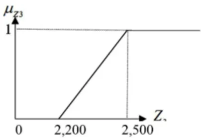
The expressions (20)-(22) are related to the maximization of the liquidity index (function Z1) under uncertainty, being adopted the values of the upper and lower limits given in Table 2:
1
max j j
j J
Z xγ
∈
=
∑
(20)1, 700 j j j J xγ ∈ ≥
∑
(21)1
l
1
l
1 1 se Z 1, 700
1, 700
, se 1,700 2, 000 2, 000 1, 700
0, se 1, 700
Z G Z Z µ ≥ − = ≤ ≤ − ≤ (22)
Figure 4 illustrates the behavior of the fuzzy goal 1 (liquidity index accumulated), being considered a linear function of triangular pertinence:
The expressions (23)-(25) are bound to the minimization of the payback (function Z2) under the situation with uncertainty, being adopted the values of the upper and lower limits given in Table 2:
2 j j j j
j J j J
Min Z xθ xτ
∈ ∈
=
∑
−∑
(23)4
j j j j
j J j J
xθ xτ
∈ ∈
− ≤
∑
∑
(24)2
2
2
2
2
1 se 4
4
, se 0 4 4 0
0, se 4 Z Z G Z Z µ ≤ − ≤ ≤ = − ≥ (25)
Figure 5 describes the behavior of the fuzzy goal 2 (total payback), as a linear triangular pertinence function:
The expressions (26)-(28) are related to the
maximization of the DTFL (function Z3) under uncertainty, being adopted the values of the upper and lower limits given in Table 2:
3 j j
j J
Max Z xρ
∈
=
∑
(26)2, 200 j j j J xρ ∈ ≥
∑
(27)3
3
3
3
3 1 if 2, 200
2, 200
, if 2,500 2, 200 2, 500 2, 200
0. if 2, 200
Z Z G Z Z µ ≥ − = ≤ ≤ − ≤ (28)
Table 2. Goals and Lower (L) and Upper (U) Bounds chosen
for the objective functions.
Goals L U
PI 1,700 1,800
TDP 1 4
DTFL 2,200 2,500
Figure 4. Function of triangular pertinence for the fuzzy
Figure 6 shows the behavior of the fuzzy goal 3 (DTFL), as a linear triangular pertinence function:
Finally, considering the data in Table 1, the FGP model can be formulated for the situation proposed by Abensur (2012):
FGP Model
Equation 29 is the objective function, which aims the maximization of the degree of achievement of the fuzzy goals associated to each objective.
i i I Max λ
∈
∑
(29)Subject to:
Hard constraints (Abensur, 2012)
Constraint 30 is the constraint that concerned to the budget use.
452, 000
j j j J
xε
∈ ≤
∑
(30)Constraints 31 to 32 are constraints to the mutually exclusive projects.
32 34 42 1
x x x
− − + ≤ (31)
19 35
13 32
1
j j
j j
x x
= =
+ ≤
∑
∑
(32)Constraint 33 is the constraint that establishes
that the total modified internal rate of return must
be higher or equal to the total minimum acceptable rate of return.
j j j j
j J j J
xη xϕ
∈ ∈
≥
∑
∑
(33)Fuzzy constraints (new)
Constraints 34 to 35 are fuzzy constraints that associate the maximization of liquidity to the goal value R$1,700.00.
1 1, 700
j j j J
xγ d−
∈
+ ≥
∑
(34)1 1 1
1 300d λ
−+ ≤ (35)
Constraints 36 to 37 are fuzzy constraints that associate the minimization of the total discounted payback to the goal value established in 4 years.
2 4
j j j j
j J j J
xθ xτ d+
∈ ∈
− − ≤
∑
∑
(36)2 2
1
1 3d λ
++ ≤
(37)
Constraints 38 to 39 are fuzzy constraints that associate the maximization of the degree of total
financial leverage to the goal value R$2,200.00.
3 2, 200
j j j J
x ρ d− ∈
+ ≥
∑
(38)3 3 1
1 200d λ
−+ ≤ (39)
Constraints 40 is the constraint associated to the domain of the variables.
{0, 1 ,} , 0, 0, 0, . 0 , .
j i i i i
x∈ ∀ ∈j J λφ≥ d+≥ d−≥ d d+ −= ∀ ∈i I (40)
Tables 3 and 4 summarize the results obtained with both models (FGP Model and Abensur Model), being highlighted that the Abensur model does not contemplate the occurrence of uncertainty and that the resolution times of the FGP model, for any scenarios, were on average 4 seconds that facilitate the generation of alternative scenarios of interest for the problem manager.
It can be observed in Tables 3 and 4 that:
• There was an increase of 380% in the number of projects selected by FGP Model (24 projects) in comparison to Abensur Model (only 05 projects). This represents that FGP Model offers a higher
flexibility to the manager;
• It was generated a higher value of PI
(= R$1,660.50) by FGP Model than by Abensur Model (PI = R$854.17), corresponding to
an increase of 94.4%. This means that the FGP model provided a better remuneration of invested capital;
Figure 5. Triangular Pertinence Function for the fuzzy goal
associated to the minimization of the total payback.
Figure 6. Triangular Pertinence Function for the fuzzy goal
• It was generated a higher value of DTFL
(= R$2,181.38) by FGP Model than by Abensur Model (DTFL = R$1,031.72), corresponding
to an increase of 111.4%. This means that the
FGP model allows a better financial turnover;
• Using FGP Model, the value of TDP (=0.02 year) was substantially lower (99.5%) than by Abensur
Model (TDP = 4.4 years), despite the occurrence
of uncertainty in the data. This means that FGP Model allows shorter time to investment recovery;
• There was a better use of the budget available (R$452,000.00) by FGP Model (investing R$446,450.00, almost 98.77% of the total resources available for investment) than by Abensur Model (investing R$149,705.00, only 33,12% of the total resources available for investment);
• The degree of achievement λi for TDP was
equal to 1.0. This means that, with the FGP
model, it was obtained a value of TDP below
the chosen fuzzy goal (4 years);
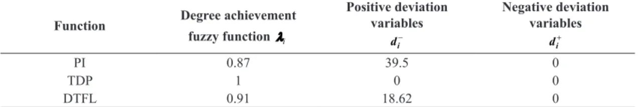
• The degree of achievement λi for PI was equal to 0.87. This means that, with the FGP Model, the value of PI was only 13% below the chosen fuzzy goal (R$1,700.00), which is fully acceptable due to the uncertainties were incorporated to the data;
• The degree of achievement λi for DTFL was equal to 0.91. This means that, with the FGP
Model, the value of DTFL was only 9% below
the chosen fuzzy goal (R$ 2,200.00), which is fully acceptable due to the uncertainties were incorporated to the data.
As an additional exercise to verify the sensitivity of the FGP model, two scenarios were generated with
respect to the requirements for PI and DTFL values. In the first scenery it was considered a decrease in
those values – it means a less strict project selection, and in the second scenery it was considered an increase in the values - it means a stricter project selection, as explained below, and the new solution results are in Tables 5 and 6:
• First scenery – the fuzzy goal for PI was decreased from R$1,700.00 to R$1,600.00 and the fuzzy
goal for DTFL was decreased from R$2,200.00
to R$2,100.00;
• Second scenery – the fuzzy goal for PI was increased from R$1,700.00 to R$1,800.00 and
the fuzzy goal for DTFL was increased from
R$2,200.00 para R$2,300.00.
As can be observed in Tables 5, for both new scenarios with uncertainty, the number of projects selected was the same previously obtained by FGP Model, i.e. 24 projects, but note that projects
6, 11 and 43 were selected only for the first scenery.
Table 3. Results of the Abensur Model and FGP model.
Item Abensur Model FGP Model Difference [%]
Number of selected
projects 5 24 380
Chosen Projects 10-12-28-35-45
1-2-3-4-5-7-10- 12-18-20-21-22-23-24-
25-26-27-28-29-30-40-41-42-45
PI [Brazilian Reais - R$] 854.17 1,660. 50 94.4
TDP [year] 4.4 years 0.02 years -99.5
DTFL [Brazilian Reais -R$] 1,031.72 2,181.38 111,4
Utilized Resources
[Brazilian Reais -R$] 149,705.00 446,450.00 198.2
Table 4. Analysis with respect to degree of achievement fuzzy functions and deviation variables values.
Function Degree achievement
fuzzy function λi
Positive deviation variables
−
i
d
Negative deviation variables
+
i
d
PI 0.87 39.5 0
TDP 1 0 0
As justification for this different selection, it is verified
that for the second scenery are selected projects with the highest goals values, which is not the case of these three projects mentioned.
In Table 5, it can be observed, also, that, although
for the first scenery has presented lower values of PI and DTFL, it presents the higher value of payback and
provides the best allocation of the available resources. Observing Table 6, for the first scenery (with uncertainty), all fuzzy goals were fully achieved (λi= 1), and it presents the best allocation (almost 99% were invested) of the available resources, while the Abensur Model proposed to invest only 33% for a situation without uncertainty.
For the second scenery, the values of PI, TDP and DTFL were the same previously got by FGP
Model, but the degree of achievement of the fuzzy
goals associated to PI and DTFL objectives were
substantially lower, respectively, 0.54 and 0.41, than those previously got by FGP Model, respectively, 0.87 and 0.91.
The sensitivity analysis shows the existence of trade-offs between objectives, enabling managers assess the impact on the solution caused by changing goals of an objective function. It also allows the
decision maker identifies which are the most important
objective functions for certain projects, for example,
for the shareholder would be desirable to maximize
profitability, and, for other hand, the company would
can be interested in to obtain the return on investment in the project in a shortest possible time.
5 Conclusions
The project selection of different nature is a very
difficult task, because usually there are many criteria
(objectives) to be optimized, the traditional investment analysis method are restricted to a mono-objective function, and they do not consider the occurrence of uncertainty. This was the main motivation to this work that used multi-objective GP models under uncertainty.
As conclusions of this paper, it can be affirmed
that the application of the FGP model was viable and relevant to solve the capital budget problem, presenting advantages in relation to the adoption of classical optimization methods (deterministic). In the case described here, the improvements found were, mainly, with regard to the increase in the number of projects included in the selected portfolio, in PI and
DTFL values, in the reduction of the payback and
in a better resources allocation.
In fact, the FGP model had a better performance
than Abensur Model, offering better PI, TDP and DTFL
values in all optimizations carried out, allowing more
Table 5. Previous and new (Sensibility Analysis) results from FGP model.
Previous results - FGP
Model First Scenery Second Scenery
Number of projects 24 24 24
Projects
1-2-3-4-5-7-10- 12-18-20-21-22-23-24-
25-26-27-28-29-30-40-41-42-45
2-3-4-5-6-7-10- 11-12-18-20-21-22-23-
24-25-26-27-28-29-30-41-42-43
1-2-3-4-5-7-10- 12-18-20-21-22-23-24-
25-26-27-28-29-30-40-41-42-45
PI [Brazilian Reais - R$] 1,660. 50 1,616.2 1,660.50
TDP [year] 0.02 0.1 0.02
DTFL
[Brazilian Reais -R$] 2,181.38 2,128.53 2,181.50
Budget
[Brazilian Reais -R$] 446,450.00 450,750.00 446,450.00
Table 6. New degree of achievement fuzzy function and deviation variables values (Sensibility Analysis).
Degree achievement fuzzy function λi
Positive deviation variables
−
i
d
Negative deviation variables
+
i
d
First Scenery
PI 1 0 0
TDP 1 0 0
DTFL 1 0 0
Second Scenery
PI 0.54 139.50 0
TDP 1 0 0
flexibility to the managers with regard to the use of
the resources, allowing testing variations in the goals. Finally, it should also be highlighted that the FGP model allows aggregating the occurrence of uncertainty in the problem of capital budget, as it is
much verified in the practice, not occasioning higher
mathematical and computational complexity both in the modeling phase and model solution, presenting low solution times.
As proposals for future researches, it is suggested to apply to the capital budget problems:
• Data Envelopment Analysis - DEA Models (Silva et al., 2013b);
• The Revised Multi-Choice Goal Programming - RCMGP- LHS (Silva et al., 2015);
• Monte Carlo simulation combined with GP models under uncertainty (Silva et al., 2014);
• Models proposed by Ekel et al. (2008) and Pereira et al. (2015) combined with GP models under uncertainty.
Acknowledgements
This research was partially supported by The
National Council for Scientific and Technological Development (CNPq - 306214/2015-6, CNPq -
431758/2016-6), São Paulo Research Foundation (FAPESP - 2015/12711-4; FAPESP- 2015/24560-0), and FAPEMIG (APQ-01188-16). We thank the contributions and suggestions from reviewers.
References
Abensur, E. O. (2012). Um modelo multiobjetivo de otimização aplicado ao processo de orçamento de capital. Gestão & Produção, 19(4), 747-758. http:// dx.doi.org/10.1590/S0104-530X2012000400007.
Abensur, E. O. (2013). Orçamento de capital: um caso especial de sequenciação de projetos. Gestão & Produção, 20(4), 979-991. http://dx.doi.org/10.1590/ S0104-530X2013000400016.
Bakirli, B. B., Gencer, C., & Aydogăn, E. K. (2013). A combined approach for fuzzy multi-objective multiple knapsack problems for defence project selection. The Journal of the Operational Research Society, 65(7), 1001-1016. http://dx.doi.org/10.1057/jors.2013.36.
Bankian-Tabrizi, B., Shahanaghi, K., & Saeed Jabalameli, M. (2012). Fuzzy multi-choice goal programming. Applied Mathematical Modelling, 35(4), 1415-1420. http://dx.doi.org/10.1016/j.apm.2011.08.040.
Bertrand, J. W. M., & Fransoo, J. C. (2002). Operations management research methodologies using quantitative
modeling. International Journal of Operations & Production Management, 22(2), 241-264. http://dx.doi. org/10.1108/01443570210414338.
Bradi, M. A., Davis, D., & Davis, D. (2000). A comprehensive 0-1 goal programming model for project selection. International Journal of Project Management, 19, 243-252.
Brigham, E. F., Gapenski, L. C., & Ehrhardt, M. C. (2001). Administração financeira: teoria e prática. São Paulo: Atlas.
Chang, C.-T. (2007). Multi-choice goal programming. Omega: International Journal of Management Sciences, 35(4), 389-396. http://dx.doi.org/10.1016/j.omega.2005.07.009.
Chang, C.-T. (2008). Revised multi-choice goal programming. Applied Mathematical Modelling, 32(12), 2587-2595. http://dx.doi.org/10.1016/j.apm.2007.09.008.
Chang, C.-T., Chen, H.-M., & Zhuang, Z.-Y. (2012a). Revised multi-segment goal programming: percentage goal programming. Computers & Industrial Engineering, 63(4), 1235-1242. http://dx.doi.org/10.1016/j.cie.2012.08.005.
Chang, C.-T., Chen, H.-M., & Zhuang, Z.-Y. (2012b). Multi-coefficients goal programming. Computers & Industrial Engineering, 62(2), 616-623. http://dx.doi. org/10.1016/j.cie.2011.11.027.
Charnes, A., & Cooper, W. W. (1961). Management model and industrial application of linear programming. New York: Wiley.
Deb, K. (2001). Multi-objective optimization using evolutionary algorithms. England: John Wiley & Sons.
Ekel, P. Y. A., Martini, J. S. C., & Palhares, R. M. (2008). Multicriteria analysis in decision making under information uncertainty. Applied Mathematics and Computation, 200(2), 501-516. http://dx.doi.org/10.1016/j. amc.2007.11.024.
General Algebraic Modeling System – GAMS. (2014). Recuperado em 28 de agosto de 2014, de http://Gams. Com/Dd/Docs/Solvers/Cplex.Pdf
Ghahtarani, A., & Najafi, A. A. (2013). Robust goal programming for multi-objective portfolio selection problem. Economic Modelling, 33, 588-592. http:// dx.doi.org/10.1016/j.econmod.2013.05.006.
Jamalnia, A., & Soukhakian, M. A. (2009). A hybrid fuzzy goal programming approach with different goal priorities to aggregate production planning. Computers & Industrial Engineering, 56(4), 1474-1486. http:// dx.doi.org/10.1016/j.cie.2008.09.010.
Khalili-Damghani, K., Sadi-Nezhad, S., & Tavana, M. (2013). Solving multi-period project selection problems with fuzzy goal programming based on TOPSIS and a fuzzy preference relation. Information Sciences, 252, 42-61. http://dx.doi.org/10.1016/j.ins.2013.05.005.
Lam, J. S. L., & Lai, H.-H. (2015). Developing environmental sustainability by ANP-QFD approach: the case of shipping operations. Journal of Cleaner Production, 105, 275-284. http://dx.doi.org/10.1016/j.jclepro.2014.09.070.
Lee, J. W., & Kim, S. H. (2000). Using analytic network process and goal programming for interdependent information system project selection. Computers & Operations Research, 27(4), 367-382. http://dx.doi. org/10.1016/S0305-0548(99)00057-X.
Li, D.-F., & Wan, S.-P. (2014). A fuzzy inhomogenous multiattribute group decision making approach to solve outsourcing provider selection problems. Knowledge-Based Systems, 67, 71-89. http://dx.doi.org/10.1016/j. knosys.2014.06.006.
Liang, G.-S., & Wang, M. J. (1993). Evaluating human reliability using Fuzzy relation. Microelectronics and Reliability, 33(1), 63-80. http://dx.doi.org/10.1016/0026-2714(93)90046-2.
Liao, C. N. (2009). Formulating the multi-segment goal programming. Computers & Industrial Engineering, 56(1), 138-141. http://dx.doi.org/10.1016/j.cie.2008.04.007.
Martel, J. M., & Aouni, B. (1998). Diverse imprecise goal programming model formulations. Journal of Global Optimization, 12(2), 127-138. http://dx.doi. org/10.1023/A:1008206226608.
Mulvey, J. M., Vanderbei, R. J., & Zenios, S. A. (1995). Robust optimization of large-scale systems. Operations Research, 43(2), 264-281. http://dx.doi.org/10.1287/ opre.43.2.264.
Pereira, J. G., Jr., Ekel, P. Y. A., Palhares, R. M., & Parreiras, R. O. (2015). On multicriteria decision making under conditions of uncertainty. Information Sciences, 324, 44-59. http://dx.doi.org/10.1016/j.ins.2015.06.013.
Romero, C. (2001). Extended lexicographic goal programming: a unifying approach. Omega, 29(1), 63-71. http://dx.doi. org/10.1016/S0305-0483(00)00026-8.
Romero, C. (2004). A general structure of achievement function for a goal programming model. European Journal of Operational Research, 153(3), 675-686. http://dx.doi.org/10.1016/S0377-2217(02)00793-2.
Saaty, T. L. (1977). A scaling method for priorities in hierarchical structures. Journal of Mathematical Psychology, 15(3), 234-281. http://dx.doi.org/10.1016/0022-2496(77)90033-5.
Saaty, T. L. (2006). Decision making with the analytic network process. International Series in Operations
Research & Management Science, 95, 1-26. http:// dx.doi.org/10.1007/0-387-33987-6_1.
Santos, A., Lavarda, C. E. F., & Marcello, I. E. (2012). The relationship between cost management knowledge and budgetary participation with managers’ performance. Revista Brasileira de Gestão de Negócios, 16, 124-142.
Santos, J. O., & Barros, C. A. S. (2011). O que determina a tomada de decisão financeira: razão ou emoção? RBGN: Revista Brasileira de Gestão de Negócios, 13(38), 7-20. http://dx.doi.org/10.7819/rbgn.v13i38.785.
Silva, A. F., & Marins, F. A. S. (2014). A Fuzzy Goal Programming model for solving aggregate production-planning problems under uncertainty: a case study in a Brazilian sugar mill. Energy Economics, 45, 196-204. http://dx.doi.org/10.1016/j.eneco.2014.07.005.
Silva, A. F., & Marins, F. A. S. (2015). Revisão da literatura sobre modelos de programação por metas determinística e sob incerteza. Production Journal, 25(1), 92-112. http://dx.doi.org/10.1590/S0103-65132014005000003.
Silva, A. F., Marins, F. A. S., & Dias, E. X. (2015). Addressing uncertainty in sugarcane harvest planning through a revised multi-choice goal programming model. Applied Mathematical Modelling, 39(18), 5540-5558. http://dx.doi.org/10.1016/j.apm.2015.01.007.
Silva, A. F., Marins, F. A. S., & Montevechi, J. A. B. (2013a). Multi-choice mixed integer goal programming optimization for real problems in a sugar and ethanol milling company. Applied Mathematical Modelling, 37(9), 6146-6162. http://dx.doi.org/10.1016/j.apm.2012.12.022.
Silva, A. F., Marins, F. A. S., & Santos, M. V. B. (2013b). Programação por metas e análise por envoltória de dados na avaliação da eficiência de plantas mundiais de manufatura. PODes, 5(2), 172-184.
Silva, A. F., Marins, F. A. S., & Silva, M. F. (2014). Otimização estocástica com múltiplos objetivos e simulação de Monte Carlo no desenvolvimento de estratégia de vendas. PODes, 6(1), 35-53.
Wang, R. C., & Liang, T. F. (2004). Projects management decisions with multiple fuzzy goals. Construction Management and Economics, 22(10), 1047-1056. http:// dx.doi.org/10.1080/0144619042000241453.
Yaghoobi, M. A., & Tamiz, M. (2007). A method for solving fuzzy goal programming problems based on MINMAX approach. European Journal of Operational Research, 177(3), 1580-1590. http://dx.doi.org/10.1016/j. ejor.2005.10.022.