www.atmos-chem-phys.net/6/2887/2006/ © Author(s) 2006. This work is licensed under a Creative Commons License.
Chemistry
and Physics
The time-space exchangeability of satellite retrieved relations
between cloud top temperature and particle effective radius
I. M. Lensky1and D. Rosenfeld2
1Department of Geography and Environmental Studies, Bar-Ilan University, Ramat-Gan, Israel 2Institute of Earth Sciences, The Hebrew University of Jerusalem, Jerusalem, Israel
Received: 30 August 2005 – Published in Atmos. Chem. Phys. Discuss.: 22 November 2005 Revised: 12 June 2006 – Accepted: 22 June 2006 – Published: 12 July 2006
Abstract. A 3-minute 3-km rapid scan of the METEOSAT Second Generation geostationary satellite over southern Africa was applied to tracking the evolution of cloud top tem-perature (T) and particle effective radius (re)of convective
elements. The evolution ofT-re relations showed little
de-pendence on time, leavingre to depend almost exclusively
onT. Furthermore, cloud elements that fully grew to large cumulonimbus stature had the sameT-re relations as other
clouds in the same area with limited development that de-cayed without ever becoming a cumulonimbus. Therefore, a snap shot ofT-rerelations over a cloud field provides the
same relations as composed from tracking the time evolu-tion ofT andre of individual clouds, and then
composit-ing them. This is the essence of exchangeability of time and space scales, i.e., ergodicity, of theT-rerelations for
convec-tive clouds. This property has allowed inference of the mi-crophysical evolution of convective clouds with a snap shot from a polar orbiter. The fundamental causes for the ergodic-ity are suggested to be the observed stabilergodic-ity ofrefor a given
height above cloud base in a convective cloud, and the con-stant renewal of growing cloud tops with cloud bubbles that replace the cloud tops with fresh cloud matter from below.
1 Introduction
Rosenfeld and Lensky (1998) introduced a technique that was used to gain insights into precipitation forming pro-cesses. This technique was applied to AVHRR data, and later to other polar orbiting sensors (VIRS on TRMM, GLI on ADEOS II, MODIS on Terra and Aqua). The Rosenfeld Lensky Technique (RLT) was used in many studies to as-sess the impact of different aerosols on clouds and precipi-tation (Rosenfeld, 1999, 2000; Rosenfeld et al., 2001, 2002,
Correspondence to:I. M. Lensky ([email protected])
2004; Rosenfeld and Woodley, 2001, 2003; Ramanathan et al., 2001; Rudich et al., 2002, 2003; Tupper et al., 2004; Williams et al., 2002; Woodley et al., 2000).
The RLT is based on two assumptions:
– The evolution of cloud top effective radius (re) with
height (or cloud top temperature, T), observed by the satellite at a given time (snapshot) for a cloud ensem-ble over an area, is similar to theT-re time evolution
of a given cloud at one location. This is the ergodicity assumption, which means exchangeability between the time and space domains.
– There near cloud top is similar to that well within the
cloud at the same height as long as precipitation does not fall through that cloud volume.
The second assumption was verified using in situ aircraft measurements (Rosenfeld and Lensky, 1998; Freud et al., 2005). This paper intends to test the ergodicity assumption using a rapid scan sequence taken by the Spinning Enhanced Visible and Infrared Imager (SEVIRI) on the European ME-TEOSAT Second Generation (MSG) geostationary satellite. To this end, rapid scan data of convective clouds over Africa is used. This paper does not intend to focus on the reasons of the different apparent behavior of clouds in different ar-eas or to associate it with aerosols, but rather to characterize systematic distinct behavior of clouds in different areas, and to show that different clouds in the same area have similar behavior and is steady with time.
2 The data
µ
-1 -0.5 0 0.5 1 1.5 2
240 250
260 270
BT
D
T
10.8Fig. 1. Temperature dependence of the BTD between 10.8 and 12.0µm channels thresholds for the cloud mask.
used to monitor convective clouds over Africa, during the pre-commissioning phase of the satellite.
Counts from the Native format data files were transformed to radiances and then to reflectances and temperatures at the solar and emissive channels respectively. The solar re-flectance component of channel 4 (3.9µm) was calculated. For the retrieval of the cloud top effective particle size, a look up table (LUT) with entries for the satellite zenith angle, so-lar zenith angle, and relative azimuth was used. The LUT was calculated using SSCR (Signal Simulator for Cloud Re-trieval) radiative transfer code (Nakajima and King, 1992; Nakajima, 1995) for optically thick clouds such that the sur-face effects can be neglected at 3.9µm (Rosenfeld et al., 2004). To make sure that only optically thick clouds are as-signed an effective radius a cloud mask was used.
The cloud mask for the retrieval ofre consists of the
fol-lowing thresholds:
– Minimum reflectance threshold of 40% at the 0.6µm channel;
– Three intervals of brightness temperature difference be-tween the 10.8 and 12.0µm channels. The first in-terval of −0.5 to 1.5 K was applied to pixels with
T10.8>260 K. The second interval of−0.5 to 1.0 K was
applied to pixels with 260>T10.8>250 K. The third
in-terval of −0.2 to 1.5 K was applied to pixels with
T10.8<250 K (see Fig. 1).
– An interval of brightness temperature difference be-tween the 10.8µm channel and the 8.7µm channel of
−1 to 5 K.
µ
µ µ
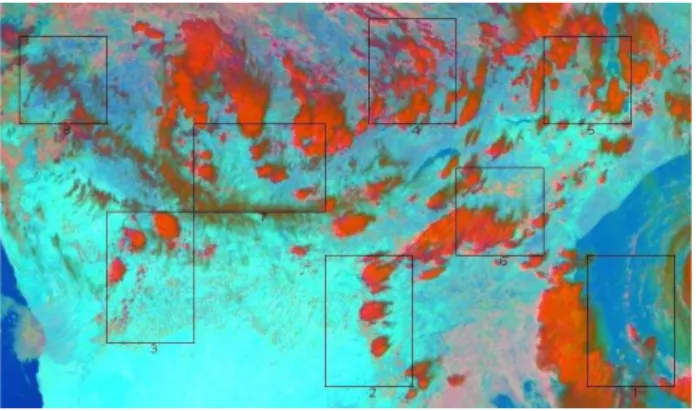
Fig. 2.MSG/SEVIRI image from 15 December 2003 13:01 GMT of convective clouds over southern Africa is shown. The color is com-posed of red for 0.8µm reflectance, green for 3.9µm reflectance (approximatingre), and blue for 10.8µm brightness temperature. The selected areas of interest for the analysis of the time-space ex-changeability of theT-reare shown.
3 Methodology
A chain of programs was applied to the MSG raw data. In the first stage pixel data (T10.8 andre)from predefined
ar-eas of interest (Fig. 2) were saved for the whole data set for further analyses. In the second stage, individual cloud cells (or convective towers) were tracked. To this end we looked for local minimum ofT10.8in a running box of 5 by 5
pix-els. The cells in each area in each time step were listed in a table. These tables included the cells’ location (line, pixel), T10.8, andre of the coldest pixel (cell center). The coldest
(highest) pixel was selected to avoid shadows from neigh-boring clouds. These shadows reduce the 3.9µm solar re-flectance, and erroneously enlarge the effective radius. In the third stage a cloud-tracking program was applied to track the individual cells with time and to give them an ID. The track-ing routine looks for the shift of the cell center between the time steps. A maximum shift of two pixels per time step was permitted. The two pixels shift enables the tracked cell to shift to a new adjacent bubble of the same cloud. This is done to allow for long enough sequences so the time evolution of theT-re plots of the individual clouds can be compared to
those of a cloud cluster composed of many clouds at differ-ent stages in their life. Finally the classicalT-replots of the
RLT for the predefined areas in Fig. 2 were saved for all the time steps.
4 Results
4.1 Time-space composition ofT-rerelations
0 5 10 15 20 25 30 35 40 -60
-50
-40
-30
-20
-10
0
10
20
Area 2
r15
r50
r85
r
eT
0 5 10 15 20 25 30 35 40
-60
-50
-40
-30
-20
-10
0
10
20
Area 3
r15
r50
r85
r
eT
0 5 10 15 20 25 30 35 40
-60
-50
-40
-30
-20
-10
0
10
20
Area 4
r15
r50
r85
r
eT
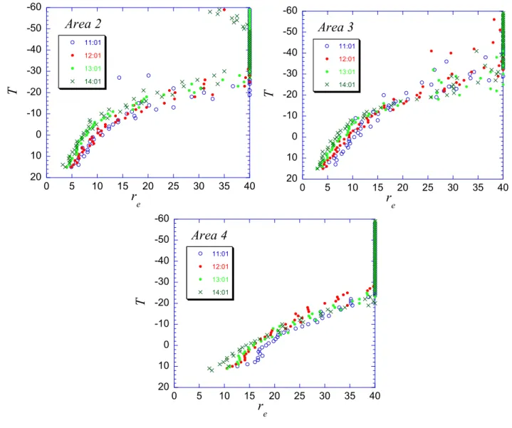
Fig. 3.Analysis of theT-rerelationship, for all the pixels that passed the cloud mask in areas 2, 3 and 4 from 13:01 GMT. Plotted are the 15th 50th, and 85th percentiles of therefor each 1◦C interval. The thick red line indicates the median, the dotted green line represent the 15th percentile, and the dotted blue line represent the 85th percentile of there. Areas 2 and 3 are microphysically continental, while area 4 is microphysically maritime.
of areas 2, 3 and 4 at 13:01 GMT. In this figure, the 15th, 50th (median) and 85th percentiles are presented. TheT-re
plots are formed by calculating the median and other per-centiles of the re for each 1◦C interval of T. If we will
examine in a certain cloud cluster (where the dynamic and thermodynamic conditions are nearly uniform) two pixels with the sameT but with differentre, than we can assume
that the pixel with the smallerre represent a more vigorous
cloud. In the supercooled water and mixed phase clouds a smallerrecan represent also a younger cloud that developed
less ice than the cloud of the second pixel. With this con-sideration in mind we can assume that the lower/higher per-centiles represent the younger/older elements at that height. In Fig. 3, the 15th percentile will represent the younger el-ements, and the 85th percentile will represent the older
ele-ments in a given height (temperature). Looking at the me-dian, the effective radius of the shallowest clouds in areas 2 and 3 is very small (re=5µm), revealing that the clouds are
microphysically continental. The effective radius of cloud droplets in these clouds pass the 15µm threshold for precip-itation (Lensky and Rosenfeld, 1997) only when the clouds develop to heights whereT10.8<−12◦C. On the other hand,
the effective radius of the shallowest clouds in area 4 is much larger (re=13µm), and it passes the 15µm threshold for
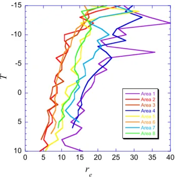
pre-cipitation atT10.8=+5◦C. Figure 4 shows medianreof all the
areas in Fig. 2 at 13:01. TheT-recurves in Fig. 4 show that
0 5 10 15 20 25 30 35 40 -10
-5
0
5
10
Area 1
Area 2
Area 3 Area 4 Area 5
Area 6 Area 7 Area 8
r
e
T
Fig. 4. The medianreof all the areas in Fig. 2 at 13:01. Areas 2, 3, and 6 are microphysically continental, areas 1 and 4 are mi-crophysically maritime, and areas 5, 7 and 8 are transition between maritime and continental.
In Fig. 5 we showT−replots of the medianreof the same
areas as in Fig. 3 at one hour intervals: 11:01, 12:01, 13:01 and 14:01 GMT. A small trend of decrease of therewith time
can be noticed in most of the areas. For example in areas 2 and 3 at T=0◦C there is a decrease of the r
e from 10µm
at 11:01 GMT to 5µm at 14:01 GMT. However it is evident from this figure that the maritime/continental behavior of the clouds in the predefined areas is clearly distinguished. For example in area 4 at the same isotherm theredecreases from
20µm at 11:01 GMT to 15µm at 14:01 GMT. The decrease of the re may be due to increased vigor of the convection
with time from morning to the afternoon, together with the increasing of cloud base height and decreasing cloud base temperature, all slowing the growth of the re with height
thus contributing to increased microphysical continentality of clouds during the day. This is manifested by the shift to the left (smallerre)of theT-replots.
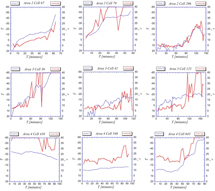
4.2 TheT-retime evolution of individually tracked clouds
Convective cloud development can be viewed as consecutive towers that dissipate or merge with previous cloud elements, and new towers replace them and develop some more, and so on until a fully-grown Cb cluster is formed in some cases, or in other cases the clouds dissipate before reaching that stature. The approach that was taken for the cloud tracking was to look for local minima of the temperature field in the cloudy pixels in each time step, and then to track these lo-cal minima from one time step to the next based on the cell
sults therefore in few long tracks along with many shorter ones that merged into the longest that made it all the way to the mature stage. It is analogous to a river (the long-tracked main cell) with many tributaries (the cells that merge to the primary one), but only one water way connects the initial de-velopment to the outlet of the river to the sea (the anvil of the mature storm). Figure 6 shows the time evolution ofT and reof these longest cloud tracks. The cells were found to be
very often regenerating in the same location, such that after a developing stage (decreasingT and increasingre), came a
drop in thereand rise of theT followed by another
develop-ing stage. For example, cell 30 in area 3 of Fig. 6 seems to glaciate after about 75 minutes (re= 40µm) but after about
5 minutesredrops to 28µm andT increases by 6◦C (from −38◦C to−32◦C). Maturation of the older glaciated cell
seg-ment may lead to thinning of the segseg-ment due to precipitation and evaporation. The resultant increase of the BTD between the 10.8 and 12.0µm channels causes these pixels to be re-jected by the cloud mask. In such case the cell track jumps to adjacent pixels that did pass the criteria of the cloud mask. Other cases like the peaks in the first 60 min of cell 30 in area 3 represent regeneration of the convective bubbles that form the cloud. These succeeding developing stages follow the generalT-recharacteristics of the area as can be seen in
Fig. 7. It follows that the general characteristicT-replot of
the area is built upon many regenerating cells that follow the sameT-rerelations (confirming again the second assumption
of the RLT).
The dynamic behaviors of single clouds were often very different; still their microphysical behavior remained consis-tent with the typicalT-replot of that area. For example, note
in Fig. 6 that cell number 41 in area 3 that do not make it to a Cb stature (lowestT >∼−20◦C) have the same r
e for
the sameT as clouds that become eventually fully grown as cell number 30 (T30=−60◦C), in spite of the dynamical
dif-ferences that determined such different fates for these two cells.
The rapid scan of the clouds microstructure allows for the first time to add the time dimension to the microphysics of clouds from space observations. The longevity of highly su-percooled (i.e., T <−10◦C) clouds tracked in Fig. 6 is 3– 4 times longer than the 10 to 15 min that were previously reported by observations made by repeated aircraft penetra-tions into tropical and subtropical microphysically continen-tal clouds (Rosenfeld and Woodley, 1997). Also the inferred updraft velocity is smaller than observations. For example, in area 2, it took about 50 min for cells number 67 and 296 to reach the re=15µm threshold (atT=−10◦C). This
0 5 10 15 20 25 30 35 40 -60
-50
-40
-30
-20
-10
0
10
20
Area 2
11:01
12:01
13:01
14:01
r
e
T
0 5 10 15 20 25 30 35 40
-60
-50
-40
-30
-20
-10
0
10
20
Area 3
11:01
12:01
13:01
14:01
r
eT
0 5 10 15 20 25 30 35 40
-60
-50
-40
-30
-20
-10
0
10
20
Area 4
11:01
12:01
13:01
14:01
r
eT
Fig. 5.Same as Fig. 3, but for the medianreat one-hour intervals: 11:00, 12:00, 13:00 and 14:00 GMT.
of the supercooled cloud water is a lot shorter than the outline of the cloud top. Furthermore, the effects of cloud drop coa-lescence to increasereand evaporation to decreaserenearly
cancel each other and cause further stability of thereas long
as the cloud is not appreciably glaciated (Freud et al., 2005). The process of the cloud top renewal by sequence of bub-bles along with the stability ofreto maturation of cloud drop
distribution at a givenT explain the apparent lack of sensi-tivity ofreto the elapsing time within the convective cloud
life cycle. The lack of time dependence ofre onT leavesre
in convective elements almost exclusively as a function ofT. This is the fundamental cause for the exchangeability of time and space, or the ergodicity of theT-rerelations.
4.3 Comparing time and space dimensions
The ergodicity assumption requires that tracking the cells and then composite back their elements should reproduce the snap shot for the cloud field to which the cells belong. This is done in Fig. 7, which shows similarT-rerelations for
cells of vastly different time evolution, some of which are presented in Fig. 6. For example, area 2 of Fig. 7 is com-posed of cell number 296 of Fig. 6, which after reaching the re=15µm threshold atT=−10◦C continued to develop for
another 20 min, reachingT=−25◦C andre=25µm, but then
started to decay, and vanished after another 20 min. It took about 20 min for cell number 30 in area 3 to cross the 0◦C isotherm, and another 50 min to start glaciate atT=−30◦C,
and vanished more then one hour later. When plotting on Fig. 7 theT-rerelations of these cell tracks while ignoring
-60 -50 -40 -30 -20 -10 0 10 20 0 5 10 15 20 25 30 35 40
0 10 20 30 40 50 60 70
T er
T [minutes] -60 -50 -40 -30 -20 -10 0 10 20 0 5 10 15 20 25 30 35 40
0 10 20 30 40 50 60
T e r
T [minutes] -60 -50 -40 -30 -20 -10 0 10 20 0 5 10 15 20 25 30 35 40
0 30 60 90 120 150
T e r
T [minutes] Area 2 Cell 296
-60 -50 -40 -30 -20 -10 0 10 20 0 5 10 15 20 25 30 35 40
0 30 60 90 120 150
T Re
T e r
T [minutes] Area 3 Cell 30
-60 -50 -40 -30 -20 -10 0 10 20 0 5 10 15 20 25 30 35 40
0 20 40 60 80 100 120
T Re
T e r
T [minutes] Area 3 Cell 41
-60 -50 -40 -30 -20 -10 0 10 20 0 5 10 15 20 25 30 35 40
0 40 80 120 160
T Re
T e r
T [minutes] Area 3 Cell 125
-60 -50 -40 -30 -20 -10 0 10 20 0 5 10 15 20 25 30 35 40
0 10 20 30 40 50 60 70 80 90 100
T Re
T e r
T [minutes] Area 4 Cell 410
-60 -50 -40 -30 -20 -10 0 10 20 0 5 10 15 20 25 30 35 40
0 10 20 30 40 50 60 70 80 90 100
T Re
T e r
T [minutes] Area 4 Cell 548
-60 -50 -40 -30 -20 -10 0 10 20 0 5 10 15 20 25 30 35 40
0 10 20 30 40 50 60 70 80 90
T Re
T e r
T [minutes] Area 4 Cell 643
Fig. 6.Time evolution ofT (dotted blue line) andre(solid red line) of the cells’ coldest pixel of some of the longer tracked convective cells in areas 2, 3 and 4.
of the areas in Fig. 3, which is repeated as the lines in the background of Fig. 7. This confirms the ergodicity of the cloud field during this case, which is all the available data so far from the pre-commissioning rapid scan of the MSG satellite.
Strictly speaking, the ergodiciy assumption is valid only for stationary conditions, i.e., not allowing systematic changes in the cloud field properties with time. However, the ergodicity approximation would be still valid if the time scale of the growing phase of convective elements is short with respect to the time scale of the changes in the cloud population properties. The time scale for growth of indi-vidual convective elements is 20 to 40 min. For example,
an air parcels would ascend at the modest updraft velocity of 5 ms−1through a 10-km deep cloud within 33 min. This time scale is much shorter than the diurnal time scale which affects the general properties of the cloud field. Therefore, the ergodiciy assumption remains generally valid, except for areas of strong gradients in the properties such as coast lines, strong aerosol gradients or over sharp transitions between different air masses.
5 Conclusions
-60
-50
-40
-30
-20
-10
0
10
20
0 5 10 15 20 25 30 35 40
Area 2
296 12:02 - 14:23
285 12:02 - 12:56
235 11:59 - 13:17
136 11:23 - 11:53 115 11:14 - 11:53 110 11:14 - 11:44 90 11:05 - 11:50 79 11:02 - 11:56
67 10:56 - 11:56
39 10:32 - 11:05
T
r
e-60
-50
-40
-30
-20
-10
0
10
20
0 5 10 15 20 25 30 35 40
Area 3
30 10:29 - 12:59
41 10:32 - 12:29
125 11:08 - 13:56
157 11:14 - 11:59 202 11:23 - 11:59 229 11:26 - 11:56 231 11:26 - 12:23 244 11:29 - 11:59
305 11:44 - 12:32
304 11:38 - 12:29
T
r
e-60
-50
-40
-30
-20
-10
0
10
20
0 5 10 15 20 25 30 35 40
Area 4
323 10:50 - 12:44
387 11:02 - 13:26
410 11:05 - 12:38
469 11:17 - 11:56 536 11:29 - 13:02 548 11:32 - 13:02 617 11:49 - 13:58 643 11:53 - 13:20
739 12:17 - 12:47
809 12:29 - 13:11
T
r
eFig. 7.Scatter plot of theT-reof the coldest pixel in some of the convective cells in areas 2, 3 and 4. Some of these cells are shown in Fig. 6. The cell number as well as the starting and ending time of the cells is displayed. An overlay of the median (thick solid line), the 15th (thin solid line) and the 85th (dotted line) percentiles of 11:01 (red) and 14:01 (blue) are added.
cloud elements in different areas. It has been shown here that individual clouds follow the general pattern of theT-re
plot that characterizes the convective cloud cluster in its spe-cific area, although the individual clouds may be very differ-ent dynamically. The single clouds, each in its stage: young, mature or dissipating, join to build theT-replot of the
clus-ter. We showed that the rate and duration of processes such as
diffusional growth and duration of supercooled phase could be inferred from the time sequence, but their variation in du-ration has little effect on the dependency ofre on T. The
resultantT-re relations of a convective cloud field is stable
curs at much longer time scales than the lifecycle times of the individual cloud elements, and hence does not violate the er-godicity assumption. Furthermore, this supports the validity of using of the ergodicity assumption for detecting variability in theT-rerelations for a cloud field under relatively slowly
varying conditions.
The validity of the ergodicity assumption is at the basis of the inference of vertical microphysical evolution of convec-tive cloud elements, using a snap shot of convecconvec-tive cloud field (Rosenfeld and Lensky, 1998). This is important be-cause of the much greater resolution of polar satellites that can take only snap shots. The validation of the ergodicity assumption provides a more solid basis for using these satel-lites snap shots for inferring the microphysical evolution of growing convective cloud elements.
Acknowledgements. The authors thank EUMETSAT for providing the unique MSG rapid scan data set that made this study possible. This study was partially supported by the Israeli Ministry of Science.
Edited by: Y. Balkanski
References
Freud, E., Rosenfeld, D., Andreae, M. O., Costa, A. A., and Artaxo, P.: Robust relations between CCN and the vertical evolution of cloud drop size distribution in deep convective clouds, Atmos. Chem. Phys. Discuss., 5, 10 155–10 195, 2005.
Lensky, I. M. and Rosenfeld, D.: Estimation of precipitation area and rain intensity based on the microphysical properties retrieved from NOAA AVHRR data, J. Appl. Meteor., 36, 234–242, 1997. Nakajima, T. and King, M. D.: Asymptotic theory for optically
thick layers, Appl. Opt., 31, 7669–7683, 1992.
Nakajima, T. Y. and Nakajima, T.: Wide-area determination of cloud microphysical properties from NOAA AVHRR measure-ments for FIRE and ASTEX regions, J. Atmos. Sci., 52, 4043– 4059, 1995.
Ramanathan, V., Crutzen, P. J., Kiehl, J. T., and Rosenfeld, D.: Aerosols, Climate and the Hydrological Cycle, Science, 294, 2119–2124, 2001.
Rosenfeld, D. and Lensky, I. M.: Satellite-based insights into pre-cipitation formation processes in continental and maritime con-vective clouds, Bull. Amer. Meteor. Soc., 79, 2457–2476, 1998.
forest fires inhibiting rainfall, Geophys. Res. Lett., 26, 3105– 3108, 1999.
Rosenfeld, D: Suppression of rain and snow by urban and industrial air pollution, Science, 287, 1793–1796, 2000.
Rosenfeld, D., Rudich, Y., and Lahav, R.: Desert dust suppressing: A possible desertification feedback loop, Proc. Natl. Acad. Sci. USA, 98, 5975–5980, 2001.
Rosenfeld, D. and Woodley, W. L.: Cloud microphysical obser-vations relevance to the Texas cold-cloud conceptual seeding model, J. Wea. Mod., 29, 56–68, 1997.
Rosenfeld, D. and Woodley, W. L.: Pollution and Clouds. Physics World, Institute of Physics Publishing LTD, Dirac House, Tem-ple Back, Bristol BS1 6BE, UK, February 2001, 33–37, 2001. Rosenfeld, D., Lahav, R., Khain, A. P., and Pinsky, M.: The role
of sea-spray in cleansing air pollution over ocean via cloud pro-cesses, Science, 297, 1667–1670, 2002.
Rosenfeld, D. and Woodley, W. L.: Closing the 50-year circle: From cloud seeding to space and back to climate change through precipitation physics, Chapter 6 of “Cloud Systems, Hurricanes, and the Tropical Rainfall Measuring Mission (TRMM)”, edited by: Tao, W.-K. and Adler, R., 234pp., p. 59–80, Meteorological Monographs 51, AMS, 2003.
Rosenfeld, D., Cattani, E., Melani, S., and Levizzani, V.: Consider-ations on daylight operation of 1.6µm vs. 3.7µm channel on NOAA and METOP Satellites, Bull. Amer. Meteor. Soc., 85, 873–881, 2004.
Rudich, Y., Rosenfeld, D., and Khersonsky, O.: Treating clouds with a grain of salt, Geophys. Res. Lett., 29(22), doi:10.1029/2002GL016055, 2002.
Rudich, Y., Sagi, A., and Rosenfeld, D.: Influence of the Kuwait oil fires plume (1991) on the microphysical development of clouds, J. Geophys. Res., 108(D15), 4478, doi:10.1029/2003JD003472, 2003.
Schmetz, J., Pili, P., Tjemkes, S., Just, D., Kerkmann, J., Rota, S., and Ratier, A.: An Introduction to Meteosat Second Generation (MSG), Bull. Amer. Meteor. Soc., 83, 977–992, 2002.
Tupper, A., Oswalt, J. S., and Rosenfeld, D.: Satellite and radar analysis of the “volcanic” thunderstorms at Mt Pinatubo, Philippines, 1991, J. Geophys. Res., 110, D09204, doi:10.1029/2004JD005499, 2004.
Williams, E., Rosenfeld, D., and Madden, M.: Contrast-ing convective regimes over the Amazon: Implications for cloud electrification, J. Geophys. Res., 107(D20), 8082, doi:10.1029/2001JD000380, 2002.