www.atmos-chem-phys.net/12/3045/2012/ doi:10.5194/acp-12-3045-2012
© Author(s) 2012. CC Attribution 3.0 License.
Chemistry
and Physics
Evaluating WRF-Chem aerosol indirect effects in Southeast Pacific
marine stratocumulus during VOCALS-REx
P. E. Saide1, S. N. Spak1, G. R. Carmichael1, M. A. Mena-Carrasco2, Q. Yang3, S. Howell4, D. C. Leon5, J. R. Snider5, A. R. Bandy6, J. L. Collett7, K. B. Benedict7, S. P. de Szoeke8, L. N. Hawkins9, G. Allen10, I. Crawford10, J. Crosier10, and S. R. Springston11
1Center for Global and Regional Environmental Research (CGRER), University of Iowa, Iowa City, Iowa, USA 2Center for Sustainability Research, Universidad Andr´es Bello, Santiago, Chile
3Pacific Northwest National Laboratory, Richland, WA, USA
4Department of Oceanography, University of Hawaii at Manoa, Honolulu, USA
5Department of Atmospheric Science, University of Wyoming, Laramie, Wyoming, USA 6Department of Chemistry, Drexel University, Philadelphia, PA, USA
7Colorado State University, Department of Atmospheric Science, Fort Collins, CO, USA
8Oregon State University, College of Earth, Ocean, and Atmospheric Sciences, Corvallis, OR, USA 9Harvey Mudd College, Department of Chemistry, Claremont, CA, USA
10Centre for Atmospheric Science, University of Manchester, Manchester, M13 9PL, UK 11Brookhaven National Laboratory, USA
Correspondence to:P. E. Said ([email protected])
Received: 16 October 2011 – Published in Atmos. Chem. Phys. Discuss.: 4 November 2011 Revised: 9 February 2012 – Accepted: 8 March 2012 – Published: 29 March 2012
Abstract. We evaluate a regional-scale simulation with the WRF-Chem model for the VAMOS (Variability of the American Monsoon Systems) Ocean-Cloud-Atmosphere-Land Study Regional Experiment (VOCALS-REx), which sampled the Southeast Pacific’s persistent stratocumulus deck. Evaluation of VOCALS-REx ship-based and three air-craft observations focuses on analyzing how aerosol loading affects marine boundary layer (MBL) dynamics and cloud microphysics. We compare local time series and campaign-averaged longitudinal gradients, and highlight differences in model simulations with (W) and without (NW) wet deposi-tion processes. The higher aerosol loadings in the NW case produce considerable changes in MBL dynamics and cloud microphysics, in accordance with the established conceptual model of aerosol indirect effects. These include increase in cloud albedo, increase in MBL and cloud heights, drizzle suppression, increase in liquid water content, and increase in cloud lifetime. Moreover, better statistical representation of aerosol mass and number concentration improves model fi-delity in reproducing observed spatial and temporal variabil-ity in cloud properties, including top and base height, droplet concentration, water content, rain rate, optical depth (COD) and liquid water path (LWP). Together, these help to quantify confidence in WRF-Chem’s modeled aerosol-cloud interac-tions, especially in the activation parameterization, while identifying structural and parametric uncertainties including:
irreversibility in rain wet removal; overestimation of marine DMS and sea salt emissions, and accelerated aqueous sulfate conversion. Our findings suggest that WRF-Chem simulates marine cloud-aerosol interactions at a level sufficient for ap-plications in forecasting weather and air quality and studying aerosol climate forcing, and may do so with the reliability required for policy analysis.
1 Introduction
Clouds play a major role in Earth’s radiative balance (Ra-manathan et al., 1989; Cess et al., 1989). However, uncer-tainties in the processes that affect cloud optical properties and modify this balance are still high (Solomon et al., 2007). These processes are driven by the indirect climatic effects of aerosols (Lohmann and Feichter, 2005), which can modify cloud albedo (Twomey, 1991) and lifetime (Albrecht, 1989), evaporate clouds (Graßl, 1979), change thermodynamics in deep convective clouds (Andronache et al., 1999), increase precipitation in ice clouds (Lohmann, 2002), and change the surface energy budget (e.g., Liepert, 2002).
generating insufficient vertical mixing, resulting in an unre-alistically shallow cloud-topped boundary layer (Otkin and Greenwald, 2008). By comparison, Large Eddy Simula-tion (LES) models have been shown to more effectively de-scribe stratocumulus clouds and their transitions (e.g., Fein-gold et al., 1998; Khairoutdinov and Kogan, 2000; Berner et al., 2011; Wang et al., 2010). Efforts have been made to couple models at both scales (regional and LES), obtaining accurate representation of stratocumulus (Zhu et al., 2010). However, operational use of these coupled models for numer-ical weather prediction (NWP) or climate studies is not yet feasible. Cloud data assimilation has been an alternative way to improve clouds in NWP (e.g., Vellore et al. 2006; Errico et al., 2007; Michel and Aulign´e, 2010).
Uncertainties in modeling aerosol indirect effects dimin-ish our capability to generate reliable climate projections, to evaluate policy questions and geo-engineering propos-als, and to provide accurate weather and air quality predic-tions. Including indirect aerosol effects has been shown to improve cloud representations in global models (Lohmann and Lesins, 2002), and a range of approaches in modeling them have been assessed (Ghan and Easter, 2006). On the regional scale, including aerosol indirect effects tends to im-pact clouds optical properties (Chapman et al., 2009) and precipitation (Ntelekos et al., 2009), and often produces bet-ter cloud representation by optical properties, dynamics and microphysics (Gustafson et al., 2007; Q. Yang et al., 2011). The LES scale has been able to show the effect on cloud structure by different cloud condensation nuclei (CCN) load-ings, and effectively simulate the dynamics of open cells, “pockets of open cells,” and closed cell marine clouds (Wang and Feingold, 2009a, b).
Intensive measurement campaigns provide a wealth of ob-servations that present the opportunity to evaluate models and to identify, quantify, and hopefully reduce these un-certainties. The VAMOS Ocean-Cloud-Atmosphere-Land Study Regional Experiment (VOCALS-REx, Wood et al., 2011) was an international field program designed to make observations of poorly understood but critical components of the coupled climate system of the southeast Pacific on the coast of Chile and Peru. Reactive gas and aerosol obser-vations show a marked longitudinal gradient from elevated values close to shore due to polluted conditions to cleaner remote conditions (Allen et al., 2011), while cloud proper-ties correlate to some extent with this gradient (Bretherton et al., 2010). Model evaluation studies emerging from the campaign have identified difficulties in accurately represent-ing MBL and stratocumulus clouds (Abel et al., 2010; Sun et al., 2010; Andrejczuk et al., 2011) without considering
In this work, we build upon previous regional simulations including aerosol feedbacks using the WRF-Chem model. Several modeling studies have performed sensitivity anal-yses of the effects of aerosol loading on cloud properties (e.g., Chen et al., 2011). Starting from a base configuration, we find another configuration that better represents aerosol mass and number concentrations, and then analyze the im-pacts of these different aerosol loading on MBL dynamics and cloud microphysics, and compare them to observations and to the canonical conceptual model of warm cloud indi-rect effects. We perform an extensive evaluation of different aspects of the model representation, and identify areas for improvements and remaining problems.
2 Methods
For the purposes of defining representative spatial zones characterized by broadly internally similar thermodynamic aerosol and composition regimes (when averaged over the length of the VOCALS-REx campaign) we choose to use the three areas as defined by Bretherton et al. (2010) and Allen et al. (2011). These are the “coastal zone” (or “off shore”, east of 75◦W), and the “remote zone” (west of 80◦W), with the two regions separated by a “transition zone” near the 78◦W meridian (75◦W–80◦W).
2.1 WRF-Chem model configuration
The WRF-Chem model simulates meteorology and atmo-spheric constituents, as well as their interactions (Skamarock et al., 2008; Grell et al., 2005). We configured WRF-Chem v3.3 with a combination of model structures, para-metric choices, and input data to best represent marine stra-tocumulus conditions, atmospheric chemistry, and secondary aerosols, with the goal of future use in meteorological and air quality forecasting.
resolution was chosen to reduce MBL and cloud height un-derestimation. The first few levels are as in Saide et al. (2011) with∼10 m thickness, and the average vertical layer spacing between 60 m and 3 km is∼60 m. In preliminary testing, this resolution produced accurate MBL and cloud heights for all longitudes, which were∼100–300 m greater than the 39-level resolution used in Saide et al. (2011).
Model structure was configured to combine modules in-cluded in contemporary WRF-Chem public release code that best represent known aerosol, cloud, and MBL processes and their couplings. Wherever possible, the most complete repre-sentations of complex physical and chemical processes were chosen. This application requires a boundary layer closure scheme that can make use of (and maintain numerical stabil-ity at) high vertical resolution, and can accurately represent the diurnal evolution of the MBL at low wind speeds. Mellor-Yamada type schemes have generally exhibited good cloud representation under these conditions (Otkin and Greenwald, 2008; Zhu et al., 2010; Rahn and Garreaud, 2010). The MYNN level 2.5 scheme (Nakanishi and Niino, 2004) was chosen since it performed well in prior applications at this resolution over Chile (Saide et al., 2011). The Lin micro-physics scheme (Chapman et al., 2009) and Goddard short wave radiation (Chou et al., 1998; Fast et al., 2006) were chosen to support aerosol direct, indirect, and semi-direct feedbacks to meteorology. Activation of aerosols from the interstitial to the cloudborne “attachment state” (Ghan and Easter, 2006) is based on a maximum supersaturation deter-mined from a Gaussian spectrum of updraft velocities and the internally mixed aerosol properties within each aerosol size bin (Abdul-Razzak and Ghan, 2002). The updraft ve-locity distribution is centered in the model vertical wind component plus the subgrid vertical velocity diagnosed from vertical diffusivity. No cumulus scheme was used follow-ing the recommendation of Q. Yang et al. (2011). The RRTM longwave radiation scheme (Mlawer et al., 1997) was used. Gases and aerosols were simulated using the CBMZ gas-phase chemical mechanism (Zaveri et al., 1999; Fast et al., 2006) with dimethyl sulfide (DMS) reactions cou-pled to the 8-bin sectional MOSAIC (Zaveri et al., 2008) aerosol module. Seawater DMS concentration was set to 2.8 nM, following the VOCA Modeling Experiment Specifi-cation (http://www.atmos.washington.edu/∼mwyant/vocals/
model/VOCA Model Spec.htm) and in agreement with mea-surements during VOCALS-REx (Hind et al., 2011). DMS is transferred to the air using sea-air exchange as in Liss and Merlivat (1986).
We chose emissions and chemical boundary conditions to best resolve spatial and temporal variability in aerosols and their precursors, taking into account a complete range of nat-ural and anthropogenic emissions sources. Continental emis-sions of biogenic trace gases (e.g., isoprene) were predicted hourly by the MEGAN algorithm (Guenther et al., 2006), and daily biomass burning locations and fuel loadings were obtained from FIRMS MODIS fire detections (Davies et al.,
2009) and modeled hourly using WRF-Chem’s plume rise model (Freitas et al., 2006, 2007). Volcanic and anthro-pogenic emissions, including point and area sources, were taken from the VOCA inventory described in detail by Mena-Carrasco et al. (2012). Table 1 shows a summary of the sources of information for the emission inventories com-piled for this research. In cases where particulate matter (PM) was not speciated, 10 %, 30 % and 70 % were associ-ated to elemental carbon, organic carbon and crustal aerosol, respectively. Chemical boundary conditions are obtained from 6-hourly MOZART global simulations (Emmons et al., 2010). MOZART fields were found to overestimate near-shore concentrations, so the model was started from clean initial conditions and spun up for 6 days to avoid biasing results. MOZART sulfur dioxide (SO2) boundary condi-tions in the free troposphere (FT) were found to be under-estimated, so a global minimum background level of 30 ppt and a 50 ppt minimum for heights over 3.5 km were set, in agreement with flight profile measurements in the remote re-gion (Allen et al., 2011; Kazil et al., 2011). Sea salt aerosol emissions were modeled following Gong et al. (1997), but resultant concentrations from the default scheme were found to substantially overestimate ship-based measurements from the NOAA RV Ronald H. Brown (Ron Brown). In order to avoid misleading indirect effects due to these biases, submi-cron emissions were reduced by a factor of 10 and super-micron emissions were reduced by a factor of 2, in line with campaign-averaged observations from the Ron Brown. De-fault WRF-Chem sea salt emissions do not consider sulfate coming from seawater, speciating sea salt as Na and Cl only. Wind-blown dust was not modeled, due to known high biases in WRF-Chem’s online wind-blown dust emissions, concen-trations, and resultant aerosol optical depth over land, and poor model representation of Andean dust composition. No organic sea emissions were considered in this study, as there was little to no evidence of these submicrometer particles during the campaign (Shank et al., 2012). Also, no secondary organic aerosols (SOA) were modeled as the fraction of SOA to total organic aerosol is thought to be low in this region (∼10 %, Kanakidou et al., 2005). New particle formation is modeled by the Wexler et al. (1994) scheme.
region NOx, SOx, VOCs,
NH3
Metropolitan region
Residential sources Chilean Ministry of environment DICTUC (2007)
PM10, PM2.5, CO,
NOx, SOx, VOC,
NH3
2005
Metropolitan region
Point sources Chilean Ministry of environment DICTUC (2007)
PM10, PM2.5, CO,
NOx, SOx, VOC,
NH3
2005
Rest of Chile Power plant emissions
Chilean power plant emissions standard KAS (2009)
PM10, PM2.5, CO,
NOx, SOx, VOC,
NH3
2009
Rest of Chile Smelter emissions Chilean air quality standards revision Mena-Carrasco (2010)
PM10, PM2.5, CO,
NOx, SOx, VOC,
NH3
2010
Rest of Chile Mobile sources SECTRA regional Corval´an et al. (2005)
PM10, PM2.5, CO,
NOX, VOC
2005
Rest of domain Total anthropogenic ex-cluding power and smelting
EDGAR 3.2 Olivier et al. (1994)
PM10, PM2.5, CO,
NOx, SOx, VOC,
NH3
2005
Rest of domain Total anthropogenic Bond et al. (2004) Black carbon and or-ganic carbon
2005
We found that aerosol wet deposition has a large influ-ence over the modeling results. In the present version of WRF-Chem, in- and below-cloud wet removal of gases and aerosols in CBMZ-MOSAIC are modeled following Easter et al. (2004). This mechanism assumes that the removal processes are irreversible, and does not consider aerosol re-suspension due to rain evaporation. This becomes an im-portant issue for the Southeast Pacific during Austral spring, since most of the drizzle observed during VOCALS-REx evaporated before reaching the surface (Bretherton et al., 2010), leading to a great contrast between cloud base and surface rain rates. Thus, irreversible removal of aerosol by rain might create an unrealistically strong sink, which is sup-ported by previous modeling results (Q. Yang et al., 2011). Kazil et al. (2011) implemented wet removal considering rain evaporation, but for a different modal aerosol approach and in the context of LES simulations. To assess the importance of modeled wet removal processes, we performed simula-tions where wet deposition was excluded, which results in higher aerosol loadings. This represents an upper limit to below cloud aerosol, and reflects the fact that low rain rates were observed at the sea surface (0.01 mm h−1on average) during the VOCALS campaign (M. Yang et al., 2011), indi-cating that most rain evaporated before reaching the surface (Bretherton et al., 2010), suggesting nearly zero wet deposi-tion. Thus, by turning off wet deposition the unrealistic sink of aerosol mass generated by not considering resuspension is removed. However, the effects in terms of number concen-tration are uncertain due to complex interactions: one droplet
can collect thousands of particles by collision-coalescence but, as some have observed (Mitra et al., 1992; Feingold et al., 1996), only one aerosol is released after evapora-tion. Since rain rates increase as aerosol number concen-tration decrease, a cloud-scavenged ultra-clean layer can be generated which can lead to conditions of particle nucle-ation (Kazil et al., 2011) potentially recovering the number of particles lost before. Without an aerosol module that in-cludes reversible wet deposition, and for the sake of study-ing the sensitivity to different aerosol loads, both simulations were conducted for the whole period. The simulation with wet deposition turned on is hereafter referred as the base run or “W”, while the simulation without wet deposition is called “NW”. Since W represents large aerosol removal, while NW no aerosol removal, we hypothesize that a model with a correct wet deposition scheme should be bounded by these two states.
2.2 Observations
be found in Benedict et al. (2012). The University of Wyoming 94 GHz cloud radar (WCR) aboard C-130 provided radar reflectivities, which were then corrected (Bretherton et al., 2010) and converted to rainfall esti-mates using the Z-R relationship described in Comstock et al. (2004). This presents results consistent with Particle Measuring Systems (PMS) Two Dimensional Cloud Probe (2D-C) probe rainfall estimates during VOCALS (Brether-ton et al., 2010). The WCR, along with an upward-pointing lidar (WCL) provided cloud top and base height estimates from the C-130 (Bretherton et al., 2010). Cloud top and base heights from Ron Brown were estimated using a millimeter-wave cloud radar (MMCR) and a Vaisala CL31 ceilome-ter, respectively (de Szoeke et al., 2010). Capping inversion height (CIH) was estimated as the height at which the tem-perature was a minimum, provided the relative humidity was at least 45 % (Jones et al., 2011) in both Ron Brown sound-ings (Wood et al., 2011) and aircrafts vertical profiles. C-130 Gerber PVM-100 Probe cloud water content, PMS Cloud Droplet Probe (CDP) and Forward Scattering Spectrometer Probe (FSSP-100) cloud droplet number concentration, and PMS Passive Cavity Aerosol Spectrometer Probe (PCASP) accumulation mode aerosol number concentration observa-tions used are described in Kazil et al. (2011) and Brether-ton et al. (2010). BAe-146 cloud and accumulation mode aerosol measurements (Allen et al., 2011) were performed with similar instruments as in C-130 (Droplet Measurement Technologies (DMT) CDP-100, PCASP) while G-1 (Klein-man et al., 2012) used a DMT Cloud and Aerosol Sampling (CAS) probe and a PCASP, respectively. An intercompari-son of the cloud microphysics probes fitted to BAe-146 and C-130 was performed on 31 October 2008 and 4 Novem-ber 2008. The aircraft performed straight and level runs (of the order of 10’s of km in length) through the same region of cloud approximately 5 min apart, finding that the num-ber concentration, LWC and size distributions were simi-lar within calibration and systematic error. However, G-1 cloud microphysics measurements showed inconsistencies compared to other probes used (Kleinman et al., 2012) prob-ably due to shattering of drizzle on CAS inlet (McFarquhar et al., 2007). On the Ron Brown, total number of particles over 13 nm was measured with a TSI 3010 Condensation Par-ticle Counter. Cloud optical depth (COD), cloud liquid water path (LWP) and cloud effective radius were obtained from MODIS-Aqua retrievals.
2.3 Performance statistics
We present box and whisker plots of longitudinal profiles at 20◦S (e.g., Fig. 1) in order to assess model performance in a consistent manner across trace gas, aerosol, and cloud prop-erties, and to focus evaluation on the longitudinal gradients identified in VOCALS-REx observations as the most impor-tant characteristics of aerosol and low cloud regimes in the Southeast Pacific (Allen et al., 2011; Bretherton et al., 2010).
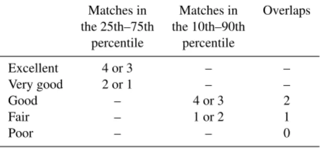
Table 2.Measure of model performance using data obtained from a box and whisker plot. A “match” is defined as a model (observa-tion) median or mean being in between the two percentiles of the observation (model) distribution. Matches ranges from 4 (perfect match) to 0 (no match). An “overlap” is defined as when mod-eled and observed inner quartiles (boxes) or inner deciles (whiskers) overlap. Overlaps ranges from 2 to 0. The final performance is assigned as the best of the three criteria.
Matches in Matches in Overlaps the 25th–75th the 10th–90th
percentile percentile
Excellent 4 or 3 – –
Very good 2 or 1 – –
Good – 4 or 3 2
Fair – 1 or 2 1
Poor – – 0
Here, we introduce a measure of accuracy deduced from these plots, hereafter referred to as the Box and Whiskers (BoW) metric and summarized in Table 2. We define a “match” as a model (observation) median or mean falling between the two prescribed percentiles of the observation (model) distribution. The first criterion (Table 2, column 1) uses the 25th and 75th percentiles (boxes in Fig. 1) and the second criterion (Table 2, column 2) uses the 10th and 90th percentiles (whiskers in Fig. 1). The third criterion (Ta-ble 2, column 3) is based on overlapping of the 25th and 75th (box overlapping) and 10th and 90th (whisker overlap-ping) percentile distributions. The net level of accuracy is determined from the sum of these three criteria, which is converted into a qualitative category: excellent, very good, good, fair and poor. Some of the advantages of the BoW method are that: it is independent of the variable being as-sessed; no absolute threshold of accuracy is specified for any variable; it is based on basic statistical parameters; it can eas-ily be read from a box and whisker plot; and it transforms a quantitative measure of accuracy into a qualitative descrip-tion. However, some issues could be encountered when the distributions are strongly skewed, as the mean could be found outside the inner quartile.
Statistics for cloud microphysics and aerosol number con-centration were computed for aircrafts profile means instead of local point to point comparisons, since observed clouds could be in different levels than model values, generating mismatches with modeled and observed clouds both present, but at different levels. For estimating the modeled 117 nm to 3 µm PCASP aerosol number concentration, values from bins 3 to 7 (156 nm to 2.5 µm) are integrated along with 42 % of the second bin (78 to 156 nm), which corresponds to the fraction over 117 nm using the logarithmic diameter.
(b)
(e) (c)
(d)
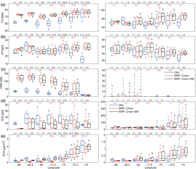
Fig. 1.Observed and modeled statistic for selected gaseous and aerosol species gridded into 2.5 degree longitudinal zones in between 22◦S and 18◦S. For each zone, centre solid (dashed) lines indicate the median (mean), boxes indicate upper and lower quartiles with upper and lower decile whiskers. The sampling time in decimal hours in each longitude bin is indicated at the top. Left column and right column are for marine boundary layer (MBL) and free troposphere (FT), respectively.
average values, while Ron Brown statistics were computed for ten minute intervals. For the case of rain statistics, model results are not filtered for missing observations and vice versa as information on rain frequency can be extracted from the total sampling time in each longitude bin on the top of the box and whisker plots (e.g., Fig. 1). This creates mi-nor inconsistencies; mainly in the 100 m height estimates, which was not measured in sub-cloud flight legs (Bretherton et al., 2010).
3 Results and discussion
We first focus on evaluating atmospheric concentrations of selected gases and aerosols for the base and NW simulations. Then, model performance is assessed for MBL dynamics and
cloud microphysics. Finally, spatial and temporal variability in chemical transport and cloud effects are investigated on an episodic basis.
3.1 Trace gas and aerosol evaluation
modeled longitudinal range with the exception of the close to the shore bin where highly polluted plumes were detected by the G-1. Measurement uncertainty is well below these differences pointing to a model bias. Neglecting these non-resolved plumes, close to shore overestimation is probably due to a lower MBL than observed (see Sect. 3.2), while re-mote zone issues are likely due to overestimation of the MBL CO MOZART boundary conditions, as these air masses of-ten had no contact with the continent for a long time period (Allen et al., 2011). However, we cannot rule out the pos-sibility that a combination of overestimates in Central Chile anthropogenic emissions (e.g., Jorquera and Castro, 2010; Saide et al., 2009) and too much entrainment in the model could generate MBL concentrations similar to FT concentra-tions. The latter case is less likely, as it would have similarly affected O3. Remote FT CO shows very good to excellent performances driven mostly by MOZART boundary condi-tions over the east-central Pacific. Even though MBL CO shows poor to fair performance in BoW metrics, differences are no more than 15 ppb, and the observed longitudinal trend (decreasing towards remote zone) and spread (<10 pbb) are often well simulated, indicating that transport in the MBL is resolved. The base and NW models show very small dif-ferences, attributable to changes in entrainment and MBL heights (see Sect. 3.2).
Figure 1b shows O3was well simulated for both the MBL and FT, with very good to excellent BoW metrics, and with similar spread. There is no clear longitudinal trend in either the model or the observations. An important point is that, as mentioned in Allen et al. (2011), the model resolves the ∼30 ppb difference between MBL and FT and also the higher variability in the FT. The lower O3in the MBL is the result of chemical destruction during the day, transport from FT during the night due to entrainment (M. Yang et al., 2011), and lower photolysis rates and temperatures under the cloud deck. Due to the ability of the model to correctly maintain the MBL to FT O3difference, we surmise that entrainment is simulated effectively. Hydroxyl radical (OH) in VOCALS MBL was estimated by Yang et al. (2009) from the DMS budget and found to have maximum diurnal values of 3–5× 10⁶molecules cm−3. WRF-Chem showed OH peaks in the lower end of this range, at∼2.5–3.35×10⁶molecules cm−3. Statistics for gas and aerosol components of the sulfur cy-cle are shown in Fig. 1c–e. The C-130 measured FT DMS (Fig. 1c, right panel) was usually below the detection limit (5 ppt), as in the model. The spikes in DMS for the 75th to 90th percentile show times where the cloud top heights were>1700 m, which is better captured by NW as explained later. In general, MBL DMS has a high bias, with poor to fair BoW scores. As discussed by Q. Yang et al. (2011), this is likely related to an overestimation of DMS emissions due to overestimation of the modeled DMS ocean : atmosphere transfer velocity. Similarly to CO, and despite the emission bias, the modeled longitudinal trend is captured very well by the model. Ron Brown atmospheric DMS measurements
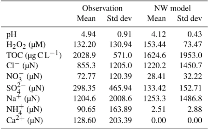
Table 3.Observed and modeled cloud chemistry statistics. Values where the observations (model) were inexistent were removed from the model (observations) statistics.
Observation NW model Mean Std dev Mean Std dev
pH 4.94 0.91 4.12 0.43
H2O2(µM) 132.20 130.94 153.44 73.47 TOC (µg C L−1) 2028.9 571.0 1624.6 1953.0 Cl−(µN) 855.3 1205.0 1220.2 1450.7 NO−3 (µN) 72.77 120.39 28.41 32.22 SO24−(µN) 298.35 465.94 133.42 152.71 Na+(µN) 1204.6 2008.6 1253.3 1486.8 NH+4 (µN) 90.65 163.89 2.51 2.88 Ca2+(µN) 128.60 203.39 0.00 0.00
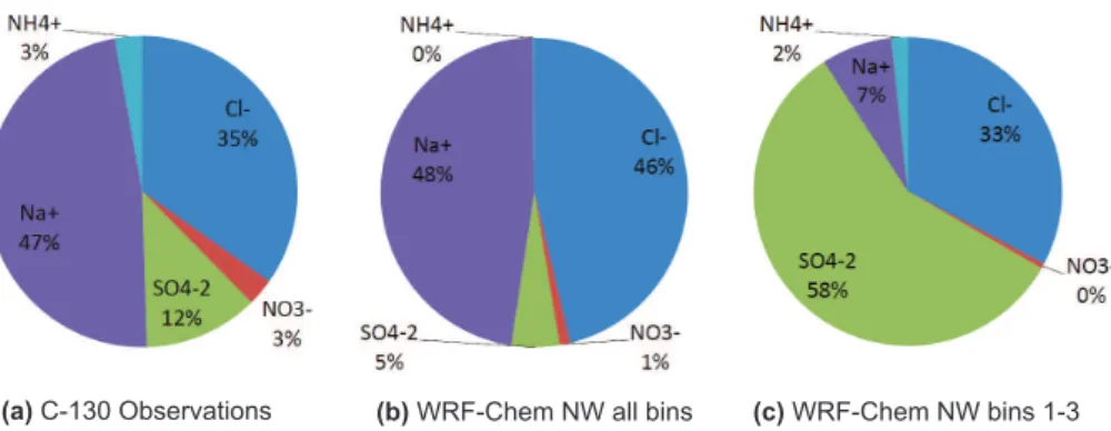
(a) C-130 Observations (b) WRF-Chem NW all bins (c) WRF-Chem NW bins 1-3
Fig. 2. Pie charts for modeled ionic species for C-130 observations representing cloud composition(a)and the no wet deposition model (NW) using collection of wet aerosol along the flight track for all bins(b)and for bin 1, 2 and 3 (40 nm to 300 nm aerosol diameter) only(c). Units are in µN.
In order to further explore SO2to sulfate conversion pro-cesses, we compare cloud chemistry observations to the NW model (Fig. 2 and Table 3), as both models show similar cloud aerosol composition. Consistent with observations (Benedict et al., 2012), model results show that bulk (sum-ming all sizes) cloud drop ion concentrations are dominated by sea salt, followed by sulfate (Fig. 2a, b). Bulk sulfate con-centrations are underestimated, since sulfate coming from seawater is not modeled. As shown by Table 3, in general the model does a good job representing the mean and vari-ability of the ion concentrations. The most notable problems are Ca+2, which is very low since no dust was modeled, and NH4, which is underestimated as it was in the AMS intersti-tial aerosol evaluation. Model pH shows the same tendency as observations, increasing towards the remote region as sul-fate aerosol is more abundant close to shore (not shown). However, model pH is always under 5, while values up to 7 were observed, leading to underprediction in mean pH (Ta-ble 3). We found that the bulk model is extremely sensitive to chloride concentrations, as a decrease in only 5 % in Cl−(as in observations) will increase average pH by 1 and increase single values up to 2.5 pH units. This is important, as WRF-Chem uses a bulk cloud chemistry scheme (Chapman et al., 2009) and small variations in Cl−(thus in pH) can generate a shift in the dominant mechanism of SO2to sulfate conver-sion, from the roughly pH independent H2O2reaction (Mar-tin and Damschen, 1981) to the O3reaction which increases in rate with pH (Hoffmann and Calvert, 1985), resulting in a speeding up of the SO2to sulfate conversion and even fur-ther reductions in SO2concentrations. However, as pointed out by M. Yang et al. (2011), most droplets nucleate from sulfate particles, so their pH will be acidic and dominated by the hydrogen peroxide reaction. This behavior for the major-ity of droplets is seen in modeled cloud water aerosol in the bins that dominate nucleation (Fig. 2c). We also see very low sea salt influence, as Na+percentage is low and Cl−is dif-fused into the droplet from HCl gas rather than entering the droplet as sea salt. All this implies that there is clear need
for sized-resolved cloud chemistry (e.g., Fahey and Pandis, 2001), and that aqueous chemistry should be considered for nucleation and accumulation modes only (Kazil et al., 2011). Measurements considering the nature of the cloud condensa-tion nuclei (CCN) composicondensa-tion and size should also be per-formed (Bator and Collett, 1997). Analyzing the H2O2 path-way, H2O2concentrations are slightly overestimated by the model (Table 3), which cannot explain the SO2gap between model and observations. M. Yang et al. (2011) found that to close the SO2 budget, the Martin and Damschen (1981) H2O2rate expression yielded best results, while other reac-tion rates were too fast to reach mass balance. We compared these rates to the McArdle and Hoffmann (1983) rates im-plemented in WRF-Chem, reaching the same answer, which could explain the difference in SO2. Another factor that in-fluences increased SO2 depletion is the consistent overesti-mation of cloud fraction, as WRF-Chem NW shows aver-age cloud fractions of 86 % on the Ron Brown track, while the MMCR on board of Ron Brown (M. Yang et al., 2011) showed values of 67 %.
3.2 MBL and marine Stratocumulus dynamics
(a)
(b)
(c)
g
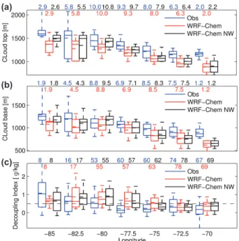
Fig. 3. Box and whisker plots for different variables derived from aircrafts measurements as in Fig. 1.(a)and(b): cloud top and bot-tom from U. of Wyoming radar (WCR) and lidar (WCL), respec-tively. (c)Decoupling index, the horizontal dashed line indicates the 0.5 g kg−1decoupling threshold (see explanation on the text). The numbers above each zone represent sampling time in decimal hours for(a)and(b), and number of profiles for(c).
when number concentration of droplets increase, precipita-tion decreases, which increases entrainment. However, this also generates extra cloud water that produces thicker clouds that absorb more shortwave radiation (lower model down-ward SW), heating the layer and decreasing entrainment. Also, when clouds rise, cloud top temperature tends to de-crease, decreasing LW cooling (model TOA outgoing LW decrease) and thus reducing entrainment. An overall increase in entrainment is achieved which cause cloud heights to rise (Pincus and Baker, 1994), in agreement with our results.
As aerosol loads increase for NW, the direct and direct effects are also expected to change. However, semi-direct effects should not play an important role as BC ob-servations (Shank et al., 2012) and model results show very low concentrations. A simulation where the aerosol radia-tion feedbacks were turned off using the NW configuraradia-tion shows small differences for cloud top pressure (<±1 %), cloud fraction (<±10 %) and water content (<±10 %), im-plying that indirect effects dominate under clean conditions like those observed during VOCALS-REx, where aerosol ra-diative effects become more important under heavily polluted conditions (Koren et al., 2008).
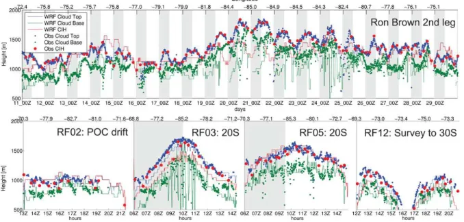
As seen in Fig. 3a, b, close to shore both simulations have large cloud height negative biases (fair to good BoW), as the coarse resolution is unable to resolve the steep topography and land-sea transition (Wang et al., 2011). In the remote
zone the NW heights captured well the observations (mostly excellent BoW classifications) while the base model under-estimated the heights (fair to excelent BoW scores). The NW model also better represents observed temperature and water vapor profiles in the remote zone both from aircraft profiles and ship-based soundings (not shown), as the typical MBL structure approaches the observed vertical profile. Even so, there are still some periods where the model does not simu-late the very high cloud heights observed in the remote zone, as depicted by the 95th extremes of the observed distribu-tion and as seen in the Ron Brown time series in Fig. 4, which are responsible for the lower model means. However, these periods of poor performance appear episodic, and there are periods where WRF-Chem NW does reach the observed heights (e.g., RF03 and RF05 on Fig. 4). Episodic under-estimation of cloud heights is thought to come from meteo-rological boundary condition issues, as the model is unable to represent the high clouds condition occurring over several days (e.g., 19–23 November). The model shows good agree-ment with observations for a range of very different condi-tions: a 20S/POC drift flight (RF02) with very thin clouds, two flights to 85 W (RF03 and RF05) with different longi-tudinal cloud trends, and a coastal pollution survey flight (RF12) capturing the latitudinal gradient in cloud height.
In order to explore the model representation of MBL dy-namics in more detail, a decoupling measure was computed. Jones et al. (2011) showed that an effective decoupling indi-cator can be calculated as the difference in total water mix-ing ratio (qt, water vapor plus cloud water) between two lev-els: 25 % and 75 % of the capping inversion height (CIH), considering a value below (above) 0.5 g kg−1 as a coupled (decoupled) MBL. Observed decoupling index and capping inversion height were obtained here from aircrafts vertical profiles following the method of Jones et al. (2011), and modeled values were obtained mapping the profiles and com-puting a modeled CIH and decoupling index. Figure 3c shows longitudinal statistics for all aircrafts flights. Both simulations represent several basic aspects of the observed decoupling. The modeled decoupling index is accurately predicted everywhere (very good to excellent BoW perfor-mance) but in the transition zone, where performance is lower but still good. On average, areas west of 78◦W are decoupled while areas east of 78◦W are coupled both in the observations and the model, and better represented by the NW simulation. The spread of the decoupling index on each zone is also well simulated, with noticeable higher spread west to 78◦W, as these zones alternate in between coupled
and decoupled MBLs. Observations show a sharp longitu-dinal transition from coupled to decoupled MBLs, which is also represented by the model.
3.3 Cloud microphysics
Fig. 4. Observed and NW model cloud bottom, cloud top and capping inversion height (CIH) time series from Ron Brown (top) and four C-130 flights (bottom). Shaded areas represent night periods.
very good to excellent (in BoW metrics) for both models (Fig. 5a), but the NW model typically shows higher amounts of cloud water than the base model as clouds are more per-manent and thicker (consistent with the Twomey effect found by Albrecht, 1989). A clear difference is seen when analyz-ing number of droplets (Fig. 5b) where the increase in cloud albedo is more evident (Twomey, 1974) and modeled inner quartiles do not overlap over the remote region. This is a re-sult of the difference in sub-cloud aerosol number concentra-tion (Fig. 5c), where not even the modeled deciles overlap. Comparing observed and model droplet number and aerosol number concentration in the remote zone, the NW model presents excellent results while the base model is biased low (poor to good BoW scores), showing vast improvements in cloud microphysics by increasing the sub-cloud aerosol to near observed levels. We found consistency in the results, as when aerosol loads are relatively close to observations, the number of droplets also becomes closer to the observations. We thus conclude that the activation routine in WRF-Chem is consistent and reliable. The inability of NW to represent the lower end and spread of the cloud droplet and aerosol num-ber distributions can be related to not considering wet depo-sition, as aerosol number is expected to decrease for intense sub-cloud rain events since a single droplet can collect a large amount of particles and release just one when evaporation occurs (Kazil et al., 2011). Close to shore overestimation of droplet number concentration by both simulations may be explained by the slight overestimation of aerosol number and also by the fact that the model finds that the aerosol num-ber concentration in the 1st bin (40 to 78 nm in diameter) is an important contributor to activated particles. The latter is
not captured by the PCASP aerosol number concentrations, as it only measures aerosol diameters over 117 nm. Free troposphere aerosol number concentration (Fig. 5d) follows the same trend as in the MBL, with good to excellent BoW accuracy and few differences between the two simulations.
(a)
(b)
(c)
(d)
g
Fig. 5. Box and whisker plots for selected cloud properties and aerosol number concentration as in Fig. 1. (a)Profile mean cloud water content. (b)Profile mean number of droplets concentration. (c)and (d): marine boundary layer (MBL) and free troposphere (FT) mean profile aerosol number concentration. Number of pro-files is indicated at the top of each longitude bin.
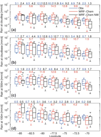
the distribution. However, modeled rain range given by the outer deciles agrees with the observations.
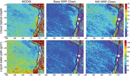
While episodic comparisons with in-situ observations are critical, it is also important to consider model performance for regional climatology, as the model should represent monthly mean values and their spatial features. Figure 7 shows COD and LWP for MODIS and both WRF-Chem sim-ulations. Model COD was computed by first computing the effective radius as in Martin et al. (1994) and then COD as proposed by Slingo (1989) for the 0.64–0.69 µm band, as the MODIS reference wavelength for this retrieval is 0.65 µm (King et al., 2006). The base WRF-Chem model usually underestimates COD, while the NW model is closer to the observations. Several features are well represented: close to shore hotspots of COD around 17◦S and 26◦S, a near-shore local COD minimum around 36S, and an increase in COD around 20◦S from 80◦W to 75◦W. In the remote zone (83◦W to 90◦W), observed COD tends to fall between both models but closer to NW, for the same reasons presented before to explain episodic performance: the base model is
(a)
(b)
(c)
(d)
Fig. 6. Box and whisker plots for radar derived and modeled rain at different heights as in Fig. 1. (a)and(b) corresponds to rain rates just below the cloud top and at the cloud base while(c)and (d)corresponds to rain rates at fixed heights of 500 and 100 m. The numbers above each zone represent sampling time in decimal hours.
unable to generate a thick enough cloud layer and drizzles too much, while the NW clouds do not dissipate when mov-ing westwards, thereby increasmov-ing cloud lifetime (Albrecht, 1989). LWP path shows a different behavior, as both models underestimate MODIS LWP, probably due to a model bias in the Lin microphysics parameterization, as the Morrison scheme (Morrison and Pinto, 2005) generates higher LWP (Q. Yang et al., 2011), as discussed further in the text. How-ever, NW model results consistently show higher values and a better agreement with observations.
3.4 Aerosol feedbacks and relation to sources
Fig. 7.MODIS-Aqua products and model monthly averages for the VOCALS period (15 October to 16 November). First and second row show cloud optical depth (COD) and liquid water path (LWP), respectively while first, second and third columns show MODIS, the base model and the no wet deposition (NW) model, respectively.
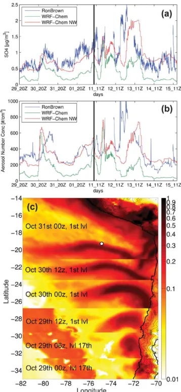
et al., 2011; Bretherton et al., 2010; Hawkins et al., 2010). To evaluate model performance and aerosol interactions, Fig. 8a compares total observed sulfate to the base and NW models. Observed values are closer to the NW model, but both mod-els resolve most of the periods where SO4concentrations in-crease over 1 µg m−3. As seen in Fig. 8b, the SO
4episodes are well correlated with aerosol number concentrations over 13 nm in diameter, a relationship also represented by the model. Observed aerosol number concentration is in the high range of the models because the lowest bin modeled is 40 nm, and does not include the 13 to 40 nm window. These sulfate episodes do not follow any diurnal pattern, and are a constant factor affecting aerosol concentrations in this zone. Model results, including prior modeling by Spak et al. (2010) that only included anthropogenic sulfur emissions, clearly indi-cate that these peaks can be attributed to continental sources, usually coming from Central Chile. As an example, Fig. 8c shows the evolution of second bin (78 to 156 nm in diame-ter) SO4(main contributor to aerosol number concentration) in a distinct pollution plume from the time emitted in Cen-tral Chile until it reaches the Ron Brown, 2 days after. When fresh, the maximum value of the plume is found on model level 17, around 650 m above sea level. At this height, it is transported by southeasterly trades (Rahn and Garreaud, 2010) until it makes contact with the MBL, where it starts entraining and SO2to SO4conversion is enhanced in clouds. Once in the MBL, lower wind speeds result in the plume tak-ing a longer time to reach the Ron Brown location. In the MBL, the plume receives additional SO4contributions from DMS, as a near-shore DMS emissions hot spot is found off central Chile (26◦S-36◦S) due to wind shear generated by
the subtropical low-level jet (Garreaud and Mu˜noz, 2005; Mu˜noz and Garreaud, 2005). By performing a simulation without DMS initial conditions and emissions, we estimate the DMS contribution to sulfate to be from 15 % to 25 % in mass (which could be overestimated as shown in previ-ous sections) by the time the plume reaches the Ron Brown location for the case analyzed, showing that these episodes are generated mainly by anthropogenic sources. The ability of these plumes to reach this zone is thought to be deter-mined by the position of the surface pressure maximum of the Southeast Pacific Anticyclone (Spak et al., 2010).
Fig. 8. (a)Time series for observed and modeled SO4. (b)Time series for observed and modeled aerosol number concentration for diameters over 13 nm and 40 nm respectively. Black thick lines in (a)and(b)divides both periods that Ron Brown stayed 4 days on 75◦W: 29 October–1 November and 11–15 November. (c) Com-posite of NW model second bin (78–156 nm aerosol diameter) SO4 concentration in µg m−3. Each composite follows the same plume since it is emitted on Central Chile until it reaches Ron Brown (marked by a circle) two days after. The two most southern compos-ites are extracted from level 17 (∼670 m over sea level) while the rest are extracted from the first model level. Scale is logarithmic.
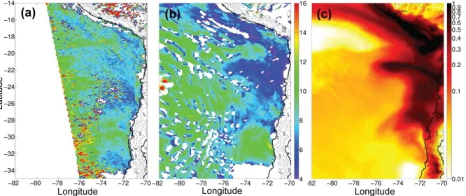
also verified by flight vertical profiles as in Fig. 3) but we still see very high precipitation gradients. Thus, differences in aerosol load might be playing a more important role than previously thought. The enhanced aerosols also participate in cloud feedbacks visible in satellite retrievals of cloud prop-erties. Figure 10a shows MODIS-Aqua cloud effective ra-dius for an overpass on a day with a thick cloud deck, where aerosol feedbacks are more pronounced. Figure 10b, c show model results for effective radius and second bin sulfate sur-face concentrations. Model cloud effective radius clearly de-creases when the MBL is dominated by high accumulation mode sulfate concentrations, following a similar shape to the plume, which can also be observed in the MODIS over-pass. The scene shows two distinct plumes coming from Central Chile: an older one between 23◦S and 20◦S and
a fresher one in between 29◦S and 25◦S, both showing a
de-crease in cloud effective radius in both model and the ob-servations. These findings highlights the need to consider aerosol interactions and transport from far-away sources in high-resolution studies and NWP applications over the re-gion and similar persistent coastal stratocumulus in eastern boundary tropical and subtropical areas.
3.5 Assessing differences due to model configuration
Fig. 9.Curtain plots for radar reflectivity (Z, in dBZ) and accumulation mode aerosol number concentration (# cm−3)for C-130 flight RF05 on 25 October.(a)and(b)shows radar observed and NW modelZwhile(c)shows NW model as the curtain and one minute average PCASP observations as colored circles. Observed Z and PCASP aerosol are 1 min averages. ModelZis computed according to Appendix A. Solid lines represent flight track with the line becoming segmented on(c)every time there is a PCASP observation. For all panels, bottom scale is time in hours and top scale is longitude in degrees.
(a)
(b)
g
Fig. 11. Results from column study for comparing Lin and Mor-rison microphysics schemes for a profile on (80◦W, 20◦S) at 00:00 UTC on 28 October 2008. (a)shows maximum rain rate per profile while(b)shows liquid water path (LWP) per profile. Each profile is run with a different droplet number concentration using a 12 s time step for enough time to reach stable conditions. For(a), missing points means rain rate equal to zero.
other hand, the Morrison scheme shows higher liquid wa-ter content (Fig. 11b), which is not completely explained by the lower precipitation, as LWP differences are still present when rain rates are similar for low number of droplets. This is also coherent with the fact that Q. Yang et al. (2011) shows better agreement to MODIS LWP than our study, where this configuration under-predicts it.
Full double moment microphysics schemes (Lin scheme is double moment for cloud water only) are necessary to im-prove process representation in models (e.g., Morrison et al., 2009). As autoconversion seems to be generating low per-formance in rain rates, we propose to implement and test the Liu et al. (2005) parameterization in the Morrison scheme. The implementation has to come along with the inclusion of aerosol re-suspension due to rain evaporation on the wet deposition scheme to avoid the MBL aerosol biases seen in Figs. 1 and 3.
4 Conclusions
There is an imperative need for reducing uncertainty and im-proving the atmospheric models used in studies of aerosol-cloud interactions at scales needed for NWP, air quality pre-dictions, and policy assessments. In this context, several intensive measurement campaigns have been carried out to improve our understanding of aerosol and cloud interactions and they provide an extensive data base for use in testing and improving models. In this work we test the regional model WRF-Chem for the VOCALS-REx campaign which focused on studying the persistent stratocumulus deck on the South East Pacific, off the shore of Chile and Peru. Start-ing from the fact that the inclusion of aerosol cloud
inter-actions in the model are important to represent processes in this region (Q. Yang et al., 2011), we perform model simula-tions designed to address the quessimula-tions: what are the effects on cloud dynamics and microphysics from changing the sub-cloud aerosol loads? And do these effects bring model results closer to observations when aerosol loads are in better agree-ment to measureagree-ments? To address these questions results from two model simulations, with (base) and without wet de-position (NW) were analyzed. Both runs represent an incom-plete modeling picture, as the base run lacks aerosol resus-pension (which is important in drizzling stratocumulus), and excluding wet deposition means neglecting a known removal process. These simulations produce significant differences in aerosol amounts, particularly in the remote zone where sulfate mass and accumulation mode aerosol number distri-butions do not overlap with each other and can be one or-der of magnitude different. Observed aerosol mass and num-ber are usually closer to the NW results, because the model wet deposition process irreversibly removes aerosol even for evaporating rain. Little surface rain was observed during the campaign, so evaporation of drizzle drops is a likely source of sub-cloud aerosols. The increase in aerosol number in NW generate a significant difference between the models in terms of marine boundary layer (MBL) dynamics and cloud microphysics, in accordance to warm clouds aerosol indirect effects. These include an increased number of cloud droplets (Twomey, 1974) showing no overlap of the inner quartiles from the two models in the remote zone; increased MBL and cloud heights (Pincus and Baker, 1994) reaching up to 200 m differences; drizzle suppression on average concen-trations and on number of detections; increased liquid water content and increased cloud lifetime (Albrecht, 1989); which helps answer the first question. MBL dynamics and cloud microphysics observed values are usually closer to NW or at least fall in between both models showing that better aerosol statistical performance lead to changes in the right direction, which helps answer the second question. This study demon-strates the capabilities of the WRF-Chem model to simulate aerosol/cloud interactions, particularly regarding the activa-tion routine, which simulates number of droplet concentra-tions more accurately when sub-cloud aerosol loads more closely match observations. However, the model needs fur-ther improvements to address issues such as aerosol resus-pension in rain wet removal, overestimation in oceanic DMS and sea-salt emissions, increased cloud driven SO2to sulfate conversion and move from bulk to sectional/modal aqueous chemistry. Also, an assessment of model differences when using distinct WRF-Chem configurations shows these seem to be related to the microphysics schemes, specifically to different autoconversion parameterizations which can gen-erate over an order of magnitude disagreement on rain rates predictions for the same conditions.
synoptic conditions with the exception of periods where the model is not able to recover from the underestimated MBL height found on the boundary conditions. Also, an episodic study was performed showing that anthropogenic sources from Central Chile substantially changed aerosol mass and number, rain and cloud optical properties over the ocean both in modeled and observed values, showing that indirect effects might be playing a more important role in modulating cloud properties and dynamics than stated in previous studies.
In our analysis we have attempted to perform a complete multi-platform evaluation for a regional simulation of clouds and aerosols, where we included VOCALS-REx observa-tions which were not compared to models previously, such as decoupling state, trace gas concentrations (carbon monox-ide, ozone), cloud aerosol composition, cloud water ionic balance and radar reflectivities. These are all crucial to fully quantifying regional model performance in this tightly cou-pled system. In order to provide quantification to this eval-uation, we introduced a new metric for assessing model per-formance that uses box and whisker plots. This metric is in-dependent of the variable being analyzed, thus allows doing performance cross-comparison in between different models and variables.
Together with improving model issues already mentioned, future work should be focused on continuing to validate mod-els with aerosol and cloud interactions from measurement campaigns in other locations, as conditions for each region vary extensively. Also, several observation platforms such as close to shore flights (NERC Dornier 228 and CIRPAS Twin Otter) and inland measurements (Iquique, Paposo and Paranal sites) were not considered as the modeling was too coarse for their use (12 km2 grid cells). Thus, finer reso-lution studies for the same area are needed to exploit these data (4–1 km2grid cells). These studies help to better quan-tify the uncertainties in models, that need to be considered when these models are used as tools for policy makers and for weather and air quality forecasts.
Appendix A
Model radar reflectivity
The Lin microphysics scheme implemented in WRF-Chem uses an exponential distribution for rain droplets (Chen and Sun, 2002):
N (D)=N0exp(−3D) (A1)
moment of the rain drop distribution as:
Z=
Z ∞
0
D6N (D)dD
which is only valid for Rayleigh scattering regime. As the radar used in this study is W-band (94 GHz frequency, ∼3 mm wavelength) then Rayleigh scattering might not be valid for droplets over 0.5 mm (O’Connor et al., 2004). In-stead, we use Mie calculations to obtainZ(Arai et al., 2005):
ZMie= λ4
π5|K|2
Z ∞
0
σMieN (D)dD (A2)
Where λ is the radar wavelength, K the absorption coef-ficient of water and σMie the backscattering cross-section, which is a function of droplet diameter and radar wavelength. Then, asN0is fixed for the Lin scheme (8e+6m4),ZMiecan be computed as a function of rain water content by numer-ically integrating this equation. For each diameter, σMie is computed using M¨atzler (2002) code which is based on the Appendix of Bohren and Huffman (1983).
Acknowledgements. We thank all people and organizations that
participated in the VOCALS-REx campaign, generating and allowing us to use the complete and comprehensive data set. Special thanks to Timothy Bates, Paquita Zuidema and Ludovic Bariteau for helping interpret and compare observational data, to William Gustafson and Jerome Fast for comments on modeling and to two anonymous reviewers for their constructive comments. Ron Brown, C-130 and G-1 measurements were obtained from the VOCALS data archive NCAR/EOL, which is sponsored by the National Science Foundation (NSF). MODIS data was obtained from the NASA Langley Research Center Atmospheric Science Data Center. Special thanks to the staff of the NCAR Research Aviation Facility for supporting the deployment of the C130 and the staff of the UWYO King Air national facility for enabling the deployment of the WCR and WCL onboard the C130 during VOCALS-REx. We also thank the UK Natural Environment Re-search Council (NERC) for funding the VOCALS UK contingent to the project (grant ref: NE/F019874/1) and the NERC Facility for Airborne and Atmospheric Measurment (FAAM) and Direct Flight and Avalon for operational support of the BAe-146 aircraft. This work was carried out with the aid of NSF grants 0748012 and 0745986, grant number UL1RR024979 from the National Center for Research Resources (NCRR), a part of the National Institutes of Health (NIH), FONDECYT Iniciaci´on grant 11090084, and Fulbright-CONICYT scholarship number 15093810. Its contents are solely the responsibility of the authors and do not necessarily represent the official views of the founding institutions.
References
Abdul-Razzak, H. and Ghan, S. J.: A parameterization of aerosol activation. 3. Sectional representation, J. Geophys. Res., 107, 4026, doi:10.1029/2001JD000483, 2002.
Abel, S. J., Walters, D. N., and Allen, G.: Evaluation of stra-tocumulus cloud prediction in the Met Office forecast model during VOCALS-REx, Atmos. Chem. Phys., 10, 10541–10559, doi:10.5194/acp-10-10541-2010, 2010.
Albrecht, B. A.: Aerosols, cloud microphysics, and fractional cloudiness, Science, 245, 1227–1230, 1989.
Allen, G., Coe, H., Clarke, A., Bretherton, C., Wood, R., Abel, S. J., Barrett, P., Brown, P., George, R., Freitag, S., McNaughton, C., Howell, S., Shank, L., Kapustin, V., Brekhovskikh, V., Klein-man, L., Lee, Y.-N., Springston, S., Toniazzo, T., Krejci, R., Fochesatto, J., Shaw, G., Krecl, P., Brooks, B., McMeeking, G., Bower, K. N., Williams, P. I., Crosier, J., Crawford, I., Con-nolly, P., Allan, J. D., Covert, D., Bandy, A. R., Russell, L. M., Trembath, J., Bart, M., McQuaid, J. B., Wang, J., and Chand, D.: South East Pacific atmospheric composition and variability sam-pled along 20◦S during VOCALS-REx, Atmos. Chem. Phys., 11, 5237–5262, doi:10.5194/acp-11-5237-2011, 2011.
Andrejczuk, M., Grabowski, W. W., Gadian, A., and Bur-ton, R.: Limited-area modelling of stratocumulus over South-Eastern Pacific, Atmos. Chem. Phys. Discuss., 11, 25517–25556, doi:10.5194/acpd-11-25517-2011, 2011.
Andronache, C., Donner, L. J., Seman, C. J., Ramaswamy, V., and Hemler, R. S.: Atmospheric sulfur and deep convective clouds in tropical Pacific: a model study, J. Geophys. Res., 104, 4005– 4024, 1999.
Arai, K., Liang, X. M., and Liu, Q.: Method for estimation of rain rate with Rayleigh and Mie scattering assumptions on theZ -Rrelationship for different rainfall types, Adv. Space Res., 36, 813–817, 2005.
Bator, A. and Collett Jr., J. L.: Cloud chemistry varies with drop size, J. Geophys. Res., 102, 28071–28078, doi:10.1029/97JD02306, 1997
Benedict, K. B., Lee, T., and Collett Jr., J. L.: Cloud water composition over the Southeastern Pacific Ocean during the VOCALS Regional Experiment, Atmos. Environ.,46, 104–114, doi:10.1016/j.atmosenv.2011.10.029, 2012.
Berner, A. H., Bretherton, C. S., and Wood, R.: Large-eddy simu-lation of mesoscale dynamics and entrainment around a pocket of open cells observed in VOCALS-REx RF06, Atmos. Chem. Phys., 11, 10525–10540, doi:10.5194/acp-11-10525-2011, 2011. Bohren, C. F. and Huffman, D. R.: Absorption of Light by Small
Particles, Wiley, New York, 1983.
Bond, T. C., Streets, D. G., Yarber, K. F., Nelson, S. M., Woo, J.-H., and Klimont, Z.: A technology-based global inventory of black and organic carbon emissions from combustion, J. Geo-phys. Res., 109, D14203, doi:10.1029/2003JD003697, 2004. Bretherton, C. S., Wood, R., George, R. C., Leon, D., Allen, G.,
and Zheng, X.: Southeast Pacific stratocumulus clouds, precip-itation and boundary layer structure sampled along 20◦S dur-ing VOCALS-REx, Atmos. Chem. Phys., 10, 10639–10654, doi:10.5194/acp-10-10639-2010, 2010.
Cess, R. D., Potter, G. L., Blanchet, J. P., Boer, G. J., Ghan, S. J., Kiehl, J. T., Le Treut, H., Li, Z. X., Liang, X. Z., Mitchell, J. F. B., and others: Interpretation of cloud-climate feedback as produced by 14 atmospheric general circulation models, Science,
245, 513–516, 1989.
Chand, D., Hegg, D. A., Wood, R., Shaw, G. E., Wallace, D., and Covert, D. S.: Source attribution of climatically important aerosol properties measured at Paposo (Chile) during VOCALS, Atmos. Chem. Phys., 10, 10789–10801, doi:10.5194/acp-10-10789-2010, 2010.
Chapman, E. G., Gustafson Jr., W. I., Easter, R. C., Barnard, J. C., Ghan, S. J., Pekour, M. S., and Fast, J. D.: Coupling aerosol-cloud-radiative processes in the WRF-Chem model: Investigat-ing the radiative impact of elevated point sources, Atmos. Chem. Phys., 9, 945–964, doi:10.5194/acp-9-945-2009, 2009.
Chen, S.-H. and Sun, W.- Y.: A one-dimensional time dependent cloud model, J. Meteorol. Soc. Japan, 80, 99–118, 2002. Chen, Y.-C., Xue, L., Lebo, Z. J., Wang, H., Rasmussen, R. M., and
Seinfeld, J. H.: A comprehensive numerical study of aerosol-cloud-precipitation interactions in marine stratocumulus, Atmos. Chem. Phys., 11, 9749–9769, doi:10.5194/acp-11-9749-2011, 2011.
Chou, M. D., Suarez, M. J., Ho, C. H., Yan, M. M. H., and Lee, K. T.: Parameterizations for cloud overlapping and short-wave single-scattering properties for use in general circulation and cloud ensemble models, J. Climate, 11, 202–214, 1998. Comstock, K. K., Wood, R., Yuter, S. E., and Bretherton, C. S.:
Re-flectivity and rain rate in and below drizzling stratocumulus, Q. J. Roy. Meteorol. Soc., 130, 2891–2918, 2004.
Corval´an, R. M., Osses, M., Urrutia, C. M., Gonzalez, P. A.: Esti-mating traffic emissions using demographic and socio-economic variables in 18 Chilean urban areas, Popul. Environ., 27, 63–87, 2005.
Davies, D. K., Ilavajhala, S., Wong, M. M., and Justice, C. O.: Fire information for resource management system: archiving and dis-tributing MODIS active fire data, IEEE T. Geosci. Remote Sens., 47, 72–79, doi:10.1109/TGRS.2008.2002076, 2009.
de Szoeke, S. P., Fairall, C. W., Wolfe, D. E., Bariteau, L., and Zuidema, P.: Surface flux observations on the southeastern tropi-cal pacific ocean and attribution of SST errors in coupled ocean-atmosphere models, J. Climate, 23, 4152–4174, 2010.
DICTUC: Actualizaci´on del Invexntario de Emisiones de Contami-nantes Atmosf´ericos en la Regi´on Metropolitana 2005, Prepared for Chilean Ministry of Environment, Santiago, Chile, 2007. Easter, R. C., Ghan, S. J., Zhang, Y., Saylor, R. D., Chapman, E. G.,
Laulainen, N. S., Abdul-Razzak, H., Leung, L. R., Bian, X., and Zaveri, R. A.: MIRAGE: Model description and evalua-tion of aerosols and trace gases, J. Geophys. Res., 109, D20210, doi:10.1029/2004JD004571, 2004.
Emmons, L. K., Walters, S., Hess, P. G., Lamarque, J.-F., Pfis-ter, G. G., Fillmore, D., Granier, C., Guenther, A., Kinnison, D., Laepple, T., Orlando, J., Tie, X., Tyndall, G., Wiedinmyer, C., Baughcum, S. L., and Kloster, S.: Description and evaluation of the Model for Ozone and Related chemical Tracers, version 4 (MOZART-4), Geosci. Model Dev., 3, 43–67, doi:10.5194/gmd-3-43-2010, 2010.
Errico, R. M., Bauer, P., and Mahfouf, J. F.: Issues regarding the assimilation of cloud and precipitation data, J. Atmos. Sci., 64, 3785–3798, 2007.
Fahey, K. M. and Pandis, S. N.: Optimizing model performance: variable size resolution in cloud chemistry modeling, Atmos. En-viron., 35, 4471–4478, 2001.
Numerical simulations of stratocumulus processing of cloud condensation nuclei through collision-coalescence, J. Geophys. Res., 101, 21391–21402, doi:10.1029/96JD01552, 1996. Feingold, G., Walko, R. L., Stevens, B., and Cotton, W. R.:
Simula-tions of marine stratocumulus using a new microphysical param-eterization scheme, Atmos. Res., 47–48, 505–528, 1998. Freitas, S. R., Longo, K. M., and Andreae, M. O.: Impact of
includ-ing the plume rise of vegetation fires in numerical simulations of associated atmospheric pollutants, Geophys. Res. Lett., 33, L17808, doi:10.1029/2006GL026608, 2006.
Freitas, S. R., Longo, K. M., Chatfield, R., Latham, D., Silva Dias, M. A. F., Andreae, M. O., Prins, E., Santos, J. C., Gielow, R., and Carvalho Jr., J. A.: Including the sub-grid scale plume rise of vegetation fires in low resolution atmo-spheric transport models, Atmos. Chem. Phys., 7, 3385–3398, doi:10.5194/acp-7-3385-2007, 2007.
Garreaud, R. D. and Mu˜noz, R. C.: The low-level jet off the west coast of subtropical South America: structure and variability, Mon. Weather Rev., 133, 2246–2261, 2005.
Ghan, S. J. and Easter, R. C.: Impact of cloud-borne aerosol rep-resentation on aerosol direct and indirect effects, Atmos. Chem. Phys., 6, 4163–4174, doi:10.5194/acp-6-4163-2006, 2006. Gong, S., Barrie, L. A., and Blanchet, J.-P.: Modeling sea salt
aerosols in the atmosphere. 1: Model development, J. Geophys. Res., 102, 3805–3818, 1997.
Graßl, H.: Possible changes of planetary albedo due to aerosol particles, in: Man’s Impact on Climate, edited by: Bach, W., Pankrath, J., and Kellogg, W., Elsevier, New York, 1979. Grell, G. A., Peckham, S. E., Schmitz, R., McKeen, S. A., Frost, G.,
Skamarock, W. C., and Eder, B.: Fully coupled “online” chem-istry within the WRF model, Atmos. Environ. 39, 6957–6975, 2005.
Guenther, A., Karl, T., Harley, P., Wiedinmyer, C., Palmer, P. I., and Geron, C.: Estimates of global terrestrial isoprene emissions using MEGAN (Model of Emissions of Gases and Aerosols from Nature), Atmos. Chem. Phys., 6, 3181–3210, doi:10.5194/acp-6-3181-2006, 2006.
Gustafson Jr., W. I., Chapman, E. G., Ghan, S. J., Easter, R. C., and Fast, J. D.: Impact on modeled cloud characteristics due to simplified treatment of uniform cloud condensation nu-clei during NEAQS 2004, Geophys. Res. Lett., 34, L19809, doi:10.1029/2007GL030021, 2007.
Hawkins, L. N., Russell, L. M., Covert, D. S., Quinn, P. K., and Bates, T. S.: Carboxylic acids, sulfates, and organosulfates in processed continental organic aerosol over the Southeast Pa-cific Ocean during VOCALS-REx 2008, J. Geophys. Res., 115, D13201, doi:10.1029/2009JD013276, 2010.
Hind, A. J., Rauschenberg, C. D., Johnson, J. E., Yang, M., and Matrai, P. A.: The use of algorithms to predict surface seawater dimethyl sulphide concentrations in the SE Pacific, a region of steep gradients in primary productivity, biomass and mixed layer depth, Biogeosciences, 8, 1–16, doi:10.5194/bg-8-1-2011, 2011. Hoffmann, M. R. and Calvert, J. G.: Chemical transformation
Jorquera, H. and Castro, J.: Analysis of urban pollution episodes by inverse modeling, Atmos. Environ. 44, 42–54, 2010.
Kanakidou, M., Seinfeld, J. H., Pandis, S. N., Barnes, I., Den-tener, F. J., Facchini, M. C., Van Dingenen, R., Ervens, B., Nenes, A., Nielsen, C. J., Swietlicki, E., Putaud, J. P., Balkan-ski, Y., Fuzzi, S., Horth, J., Moortgat, G. K., Winterhalter, R., Myhre, C. E. L., Tsigaridis, K., Vignati, E., Stephanou, E. G., and Wilson, J.: Organic aerosol and global climate modelling: a review, Atmos. Chem. Phys., 5, 1053–1123, doi:10.5194/acp-5-1053-2005, 2005.
KAS: “An´alisis General del Impacto Social y Econ´omico de la Norma de Emisi´on Para Termoel´ectricas.” Chilean Ministry of the Environment, available at: http://www.sinia.cl/1292/ articles-44963 informe final term.pdf, last access: November 2011, 2009.
Kazil, J., Wang, H., Feingold, G., Clarke, A. D., Snider, J. R., and Bandy, A. R.: Modeling chemical and aerosol processes in the transition from closed to open cells during VOCALS-REx, At-mos. Chem. Phys., 11, 7491–7514, doi:10.5194/acp-11-7491-2011, 2011.
Khairoutdinov, M. and Kogan, Y.: A new cloud physics parameteri-zation in a large-eddy simulation model of marine stratocumulus, Mon. Weather Rev. 128, 229–243, 2000.
King, M. D., Platnick, S., Hubanks, P. A., Arnold, G. T., Moody, E. G., Wind, G., and Wind, B.: Collection 005 change summary for the MODIS cloud optical property (06 OD) al-gorithm, available at: http://modis-atmos.gsfc.nasa.gov/C005 Changes/C005 CloudOpticalProperties ver311.pdf, last accesse: November 2011, 2006.
Kleinman, L. I., Daum, P. H., Lee, Y.-N., Lewis, E. R., Sedlacek III, A. J., Senum, G. I., Springston, S. R., Wang, J., Hubbe, J., Jayne, J., Min, Q., Yum, S. S., and Allen, G.: Aerosol concen-tration and size distribution measured below, in, and above cloud from the DOE G-1 during VOCALS-REx, Atmos. Chem. Phys., 12, 207–223, doi:10.5194/acp-12-207-2012, 2012.
Koren, I., Martins, J. V., Remer, L. A., and Afargan, H.: Smoke in-vigoration versus inhibition of clouds over the Amazon, Science, 321, 946–949, 2008.
Liepert, B. G.: Observed reductions of surface solar radiation at sites in the United States and worldwide from 1961 to 1990, Geo-phys. Res. Lett., 29, 1421, doi:10.1029/2002GL014910, 2002. Liss, P. S. and Merlivat, L.: Air-sea gas exchange rates: Introduction
and synthesis, in: The role of air-sea exchange in geochemical cycling, edited by: Buat-Menard, P., 113–127, 1986.
Liu, Y., Daum, P. H., and McGraw, R. L.: Size trunca-tion effect, threshold behavior, and a new type of autocon-version parameterization, Geophys. Res. Lett., 32, L11811, doi:10.1029/2005GL022636, 2005.