Use of soil moisture dynamics and patterns for the investigation of runoff generation processes with emphasis on preferential flow

(1)

HESSD

4, 2587–2624, 2007

Soil moisture dynamics and runoff

generation processes

T. Blume et al.

Title Page

Abstract Introduction

Conclusions References

Tables Figures

◭ ◮

Back Close

Full Screen / Esc

Printer-friendly Version

Interactive Discussion

EGU Hydrol. Earth Syst. Sci. Discuss., 4, 2587–2624, 2007

www.hydrol-earth-syst-sci-discuss.net/4/2587/2007/ © Author(s) 2007. This work is licensed

under a Creative Commons License.

Hydrology and Earth System Sciences Discussions

Papers published inHydrology and Earth System Sciences Discussionsare under

open-access review for the journalHydrology and Earth System Sciences

Use of soil moisture dynamics and

patterns for the investigation of runo

_ff

generation processes with emphasis on

preferential flow

T. Blume, E. Zehe, and A. Bronstert

Institute for Geoecology, Section of Hydrology and Climatology, University of Potsdam, Germany

(2)

HESSD

4, 2587–2624, 2007

T. Blume et al.

Title Page

Tables Figures

◭ ◮

Back Close

Full Screen / Esc

Abstract

Spatial patterns as well as temporal dynamics of soil moisture have a major influence

on runoffgeneration. The investigation of these dynamics and patterns can thus yield

valuable information on hydrological processes, especially in data scarce or previously ungauged catchments. The combination of spatially scarce but temporally high

resolu-5

tion soil moisture profiles with episodic and thus temporally scarce moisture profiles at additional locations provides information on spatial as well as temporal patterns of soil

moisture at the hillslope transect scale. This approach is better suited to difficult terrain

(dense forest, steep slopes) than geophysical techniques and at the same time less cost-intensive than a high resolution grid of continuously measuring sensors. Rainfall

10

simulation experiments with dye tracers while continuously monitoring soil moisture response allows for visualization of flow processes in the unsaturated zone at these

lo-cations. Data was analyzed at different spacio-temporal scales using various graphical

methods, such as space-time colour maps (for the event and plot scale) and indica-tor maps (for the long-term and hillslope scale). Annual dynamics of soil moisture

15

and decimeter-scale variability were also investigated. The proposed approach proved to be successful in the investigation of flow processes in the unsaturated zone and showed the importance of preferential flow in the Malalcahuello Catchment, a data-scarce catchment in the Andes of Southern Chile. Fast response times of stream flow indicate that preferential flow observed at the plot scale might also be of importance

20

at the hillslope or catchment scale. Flow patterns were highly variable in space but persistent in time. The most likely explanation for preferential flow in this catchment is a combination of hydrophobicity, small scale heterogeneity in rainfall due to redis-tribution in the canopy and strong gradients in unsaturated conductivities leading to self-reinforcing flow paths.

(3)

HESSD

4, 2587–2624, 2007

T. Blume et al.

Title Page

Tables Figures

◭ ◮

Back Close

Full Screen / Esc

EGU

1 Introduction

Identification of patterns of soil moisture response to rainfall and especially the vertical dynamics of soil moisture at the hillslope or plot scale can be useful for the

investiga-tion of runo_ffgeneration processes in a previously ungauged or data scarce catchment.

When investigating runoffgeneration processes in a previously ungauged catchment

5

it becomes obvious from the start that the equipment we are about to install is insuf-ficient. There will be neither enough data points in time nor in space to characterize these processes in their temporal and spatial variability. A possible way to overcome this problem is the approach where a multitude of experimental methods is applied within a relatively short time frame, producing a data set that highlights a multitude

10

of angles and aspects of catchment functioning. This type of study was carried out in the Malalcahuello Catchment in the Chilean Andes and is described in Blume et al. (2007a)1.

One important aspect of the Malalcahuello study was the question whether a combi-nation of spatially scarce soil moisture profiles with high temporal resolution, additional

15

episodic measurements of soil moisture along two hillslope transects and continuously monitored dye tracer irrigation experiments can provide useful insights into the

pro-cesses of runoffgeneration in young volcanic ash soils. The young volcanic ash soils

of Chile are little understood in their hydrological characteristics and no studies of high temporal resolution soil moisture dynamics were found in our literature search.

How-20

ever, in other parts of the world such as New Zealand or Japan the soil moisture

dy-namics of volcanic ash soils has been investigated to some extent: Hasegawa(1997)

used hourly TDR data to investigate soil water conditions and movement, Musiake

et al. (1988) used tensiometric observations and a numerical model to study infiltration

and drying behaviour of these soils andVan’t Woudt (1954) used 19 small lysimeters

25

1

(4)

HESSD

4, 2587–2624, 2007

T. Blume et al.

Title Page

Tables Figures

◭ ◮

Back Close

Full Screen / Esc

to investigate subsurface stormflow.

Soil moisture data has been used as a means to understand runo_ff generation in

other parts of the world (e.g. Kienzler and Naef, 2007; Meyles et al., 2003;

McNa-mara et al.,2005;Frisbee et al.,2007;Germann and Zimmermann,2005;Zhou et al.,

2002;Hino et al.,1988) or for the investigation of the e_ffects of changes in land use

5

or management on hydrological processes (Williams et al., 2003; Starr and Timlin,

2004). In most studies soil moisture was measured either with high spatial or with high

temporal resolution, thus producing either spatial soil moisture patterns (Bardossy and

Lehmann,1998;Brocca et al.,2007;Meyles et al.,2003;Williams et al.,2003;

West-ern et al.,2004;Rezzoug et al.,2005;Nyberg,1996) or information on the dynamics

10

(e.g. McNamara et al.,2005;Starr and Timlin,2004;Frisbee et al.,2007). A

combi-nation of both can only be achieved with either a large number of probes measuring

continuously such as inStarr and Timlin(2004) andTaumer et al. (2006) or with

geo-physical methods such as described for example inZhou et al.(2001), where electric

resistivity tomography was used to investigate soil moisture dynamics on a 3.5×3.5 m

15

plot at hourly resolution. However, the first of these two options is cost-intensive while the second is predominantly carried out on grassland, fields or bare soils with little to-pography and is not feasible in complex terrain. Combining high temporal resolution soil moisture profiles at few points in space with episodic manual measurements at

additional locations thus might be a viable cost-efficient alternative for difficult terrain.

20

At the Malalcahuello Catchment soil moisture was measured on two steep hills-lope transects. Data was collected with a data logger at high temporal resolution at three points and manually at irregular intervals at 11 additional points. Each

mea-surement produces soil moisture data for 6 different depths along a vertical profile.

While this is still a pitiful number of data points it is nevertheless possible to get a

25

general understanding of the major processes occurring within the unsaturated zone

of this catchment. Data was analyzed using different graphical methods allowing for

data exploration at different spatio-temporal scales. By carrying out rainfall

(5)

HESSD

4, 2587–2624, 2007

T. Blume et al.

Title Page

Tables Figures

◭ ◮

Back Close

Full Screen / Esc

EGU it was possible to corroborate our perception of flow in the unsaturated zone at these

locations. This combination of high temporal resolution soil moisture measurements, rainfall simulation experiments and the use of dye tracers to corroborate the conclu-sions gained from the soil moisture time series is noteworthy and only one other study (Weiler and Naef, 2003) using a slightly di_fferent layout was found in our literature

5

search. The study at the Malalcahuello catchment furthermore included the analysis of response times at the event scale, yearly soil moisture dynamics, spatial patterns and their long-term dynamics for 14 locations and 6 depths and the investigation of small scale soil moisture variability at the decimeter scale.

The four main questions of the study in the Malalcahuello Catchment were:

10

1. Can soil moisture data be used to investigate the dynamic patterns of unsaturated

flow and can these patterns be attributed to runoffgeneration processes?

2. Are moisture patterns persistent in time and space?

3. What are the causes for the observed moisture/flow patterns?

4. How important are these patterns for the entire system/catchment response?

15

2 Research area

2.1 The Malalcahuello catchment

The research area is situated in the Reserva Forestal Malalcahuello, in the Pre-cordillera of the Andes, IX. Region, Chile. The catchment is located on the south-ern slope of Volc ´an Lonquimay (38◦25.5′–38◦27′S; 71◦32.5′–71◦35′E). The catchment

20

covers an area of 6.26 km2. Elevations range from 1120 m to 1856 m above sea level,

with average slopes of 51%. 80% of the catchment is covered with forest of the

type Araucaria (Araucaria araucana) (with Lenga (Nothofagus pumilio) and Coig ¨ue

(6)

HESSD

4, 2587–2624, 2007

T. Blume et al.

Title Page

Tables Figures

◭ ◮

Back Close

Full Screen / Esc

(Nothofagus alpina) – Coig ¨ue (Nothofagus dombeyi) at lower elevations. These types

of native forest have a dense understorey of bamboo (Chusquea culeou). There is

no anthropogenic intervention. Due to this dense vegetation interception losses be-come significant: on average only 80% of total precipitation reaches the forest floor as throughfall (measured with a raster of throughfall collectors with a diameter of 10.5 cm).

5

However, throughfall amounts are highly variable and can in places also exceed total precipitation (measured outside the forest) by a factor of 2 or even 3 (Blume et al.,

2007a1). Above the tree line (20% of the catchment area) there is no significant

vege-tation cover.

The soils are young, little developed and strongly layered volcanic ash soils

(An-10

dosols, in Chile known as Trumaos) (Iroum ´e,2003; Blume et al., 2007a1). High

perme-abilities (saturated and unsaturated), high porosities (60–80%) and low bulk densities

(0.4–0.8 g/cm3) are typical for volcanic ash soils. They also usually show a strong

hys-teresis and irreversible changes (e.g. in water retention) with air-drying (Shoji et al., 1993). Soil hydraulic conductivities for the soils in the Malalcahuello catchment were

15

determined in the lab with the constant head method and range from 1.22∗10−5 to

5.53∗10−3m/s for the top 45 cm, with an average of 5.63∗10−4m/s (42 samples). The

mean conductivity for the fine gravel and pumice layers is 1.88∗10−3m/s (9 samples).

Porosities for all horizons sampled range from 56.8% to 82.1%. The mean porosity for the top 45 cm is 71.7% with a standard deviation of 6.6% (16 samples). Layer thickness

20

is also highly heterogeneous, and can range from 2–4 cm to several meters. Depth to bedrock is unknown, however manual augering to depths of 2–3 m, at one occasion

even 7 m was possible (Blume et al., 2007a1). At the locations of the 4 wells at the

lower end of this slope (Fig.1) groundwater was found in depths of 1.8–3.2 m below

the surface. However, at many other locations on this slope no groundwater was found

25

in auger holes of similar depths. Grain size distributions for the upper horizons resulted in an average of 66.5% sand, 30.4% silt and 3% clay. In the coarse layers the grain

size fraction≥2 mm ranges from 38–86% (Blume et al., 2007a1). For a more detailed

(7)

HESSD

4, 2587–2624, 2007

T. Blume et al.

Title Page

Tables Figures

◭ ◮

Back Close

Full Screen / Esc

EGU The climate of this area can be described as temperate/humid with altitudinal

ef-fects. There is snow at higher elevations during winter and little precipitation during the summer months January and February. Annual rainfall amounts range from 2000

to over 3000 mm, depending on elevation. Event runoffcoefficients are low, with 1–10

% for 17 events analyzed in 2004/2005, of which a third are smaller than 2% (Blume

5

et al.,2007c). (The method of baseflow separation used in this analysis is described

inBlume et al.,2007c.) On the other hand, yearly runoffcoefficients (>60%) as well as

the baseflow index (>75%) calculated for the years 2004 and 2005 are high (Blume et

al., 2007a1).

An overview of catchment layout and topography as well as instrumentation is given

10

in Fig.1.

3 Approach and methodology

3.1 Approach

The approach of this study is based on the measurement of spatially scarce but high temporal resolution soil moisture profiles on the one hand and additional episodic

15

and therefore temporally scarce soil moisture profiles on the other hand. These two datasets combined with additional experiments described below were used to

investi-gate different aspects of soil moisture response patterns and thus flow in the

unsatu-rated zone. These aspects included the analysis of event response patterns resulting in the deduction of flow processes, the use of rainfall simulation experiments with dye

20

tracers to corroborate these deductions, but also the analysis of response times at the event scale as well as yearly soil moisture dynamics. The episodic measurements along the hillslope transects allow for the analysis of spatial patterns and their long-term dynamics for 14 locations and 6 depths and for the investigation of small scale soil moisture variability at the decimeter scale.

(8)

HESSD

4, 2587–2624, 2007

T. Blume et al.

Title Page

Tables Figures

◭ ◮

Back Close

Full Screen / Esc

3.2 Soil moisture profiles

Soil Moisture was measured at two transects with FDR (frequency domain reflectom-etry) profile probes (Delta-T) in 10, 20, 30, 40, 60 and 100 cm depth. Both transects

are located on the eastern slope close to the main stream gauging station S1 (Fig.1).

These profile probes do not measure within a purely circular field as the sensor only

5

extends about two thirds around the probe. By taking three measurements, turning the

probe by 120◦each time, the full circle is covered. At each depth soil moisture is

mea-sured in a soil volume of about 2.5 L, a cylinder with a radius of 10 cm. The absolute measurement error of about 3% (manual of the profile probe) is for the measurement of the dynamics of soil moisture of less importance. The error of the measured dynamics,

10

i.e. the error of the values relative to each other is likely to be smaller than the absolute error. As a result of the special characteristics of the volcanic ash soil, such as the extremely high porosities and the fact that volcanic glass is a primary constituent, the built-in standard calibrations were not applicable. It was thus necessary to calibrate the probe specifically for this type of soil with gravimetrically determined water contents of

15

19 soil samples of the upper horizons.

Three profile probes were connected to a data-logger and were measuring contin-uously with a temporal resolution of 10 min. The data set extends from March 2003 to May 2006 for the lowest probe and from December 2004 to May 2006 for the two upper probes. For easier reference the three probes are numbered: probe 1 is

lo-20

cated at the lower end and probe 3 at the upper end of the hillslope transect. A fourth probe was used for manual measurements at 11 points along the transects. 5 of these measurement locations supplement the transect of the continuously measuring probes,

while the remaining 6 form the second transect located to the north of the first (Fig.1).

The points on the transects were evenly spaced. These manual measurements were

25

(9)

HESSD

4, 2587–2624, 2007

T. Blume et al.

Title Page

Tables Figures

◭ ◮

Back Close

Full Screen / Esc

EGU

3.3 Rainfall simulation experiments

By carrying out rainfall simulation experiments using a dye tracer over each of the continuously measuring probes it was possible to test our perception of flow in the unsaturated zone at these locations. The dye tracer experiments were carried out

in May 2007. The plot size was 1.2 m2 with the probe situated in the center. For

5

all experiments the dye tracer Brilliant Blue with a concentration of 4 g/l was used.

The dye was applied with a hand pressurized pesticide sprayer in order to simulate rainfall. 30 liters of the dye were sprayed over a period of 3 h. This corresponds to a

total of 25 mm at application rates of 8.3 mm/h on average. Profiles of the plots were

excavated the following day and photos of the dye patterns were taken with a digital

10

camera.

3.4 Streamflow, groundwater levels and rainfall

Water levels in stream and groundwater were measured with capacitive water level sensors (WT-HR Trutrack) at 5–10 min time intervals. Stream water levels were con-verted to discharge with the help of a rating curve. Rainfall was measured with a

15

tipping bucket rain gauge with a resolution of 0.27 mm. A climate station maintained by the Universidad Austral de Chile is located in a nearby forest plantation at 1270 m elevation. This climate station has been logging the parameters rainfall, temperature, relative humidity, wind direction and velocity as well as global radiation at hourly inter-vals since 1999. During the winter of 2005 an ultra-sonic snow height sensor was also

20

installed at this climate station. For more details on the experimental methods applied

in the Malalcahuello Catchment see Blume et al. (2007a)1.

3.5 Response times

Response times were calculated from the time series of rainfall, soil moisture,

ground-water levels at well W1 (Fig.1) and streamflow (all with 10 min resolution). Response

(10)

HESSD

4, 2587–2624, 2007

T. Blume et al.

Title Page

Tables Figures

◭ ◮

Back Close

Full Screen / Esc

time in this case was defined as the time period between begin of precipitation and first response of soil, ground- and stream water. The following threshold values were used to identify the point of first response in the time series: an increase of 0.2 Vol% in soil

moisture, an increase of 0.005 m in groundwater level and an increase of 0.01 m3/s in

stream flow.

5

3.6 Data analysis

Data was analyzed at different space-time scales using various graphical methods.

The space-time scales analyzed included event and longterm scale, point and hills-lope scale. Event scale datasets with high temporal resolution were analyzed with the help of colour maps which included temporal dynamics similar to those used by

10

Weiler and Naef(2003). Here, time is plotted on the x-axis while depth is plotted on the y-axis. Soil water content at each depth and point in time is visualized by color, chang-ing from blue to red with increaschang-ing wetness. For additional information the response of streamflow and groundwater, as well as the rainfall intensity at each point in time were also included. Color scales were adapted from one event to the next in order to

15

get the best “color resolution” possible, producing clearer patterns of response. It thus becomes possible to explore and identify patterns in moisture response, patterns in

space and time that are much more di_fficult to identify in the classical line plots of soil

moisture dynamics. In a next step flow processes were deduced from these patterns. Soil moisture patterns at the hillslope scale are investigated with the help of indicator

20

maps for each depth. These maps show locations where soil moisture is above/below a certain threshold, here the median value for that depth or the 75% quantile, respec-tively. Additionally, the temporal aspect of these patterns is also included by plotting location on the slope on the y-axis and time on the x-axis, thus giving an idea of pattern persistency.

25

(11)

HESSD

4, 2587–2624, 2007

T. Blume et al.

Title Page

Tables Figures

◭ ◮

Back Close

Full Screen / Esc

EGU

3.7 Unsaturated conductivities

In order to obtain unsaturated conductivities for the top horizons it was necessary to es-timate the Van Genuchten parameters by fitting the Van Genuchten equation to the soil moisture characteristic curves. Soil moisture characteristic curves were determined with a pressure chamber for the first two horizons below the humus layer (3 samples

5

each). The Van Genuchten parameters were then used to determine the unsaturated conductivities for a chosen matric potential.

3.8 Hydrophobicity

Potential hydrophobicity was measured with the Water Drop Penetration Time (WDPT)

test as described in Dekker and Ritsema(1994) for 12 air dried soil samples from 4

10

different locations and depths from 5 to 80 cm. The WDPT test is a simple test for water

repellency where a water drop is applied to a soil sample and the time between appli-cation of the water drop and its penetration into the soil is measured. Water drop

pene-tration times for air dried soil have been classified byDekker and Ritsema(1994) into 5

classes of water repellency: wettable (<5 s), slightly water repellent (5–60 s), strongly

15

water repellent (60–600 s), severely water repellent (600–3600 s) and extremely water

repellent (>3600 s). After testing if a soil sample was wettable soil samples showing

water repellency were submitted to 12 repetitions of the WDPT, each test carried out

with a different subsample.

4 Results and discussion

20

4.1 Soil moisture dynamics on event basis

(12)

HESSD

4, 2587–2624, 2007

T. Blume et al.

Title Page

Tables Figures

◭ ◮

Back Close

Full Screen / Esc

snow, either directly by snowfall or by rain on snow events. While snowfall will reduce the amount of water infiltrating at the time of the event, rain on snow events will have the

effects of flow on or within the snowcover as well as infiltration of meltwater. However,

as snow water equivalent was not measured, these effects could not be measured

directly.

5

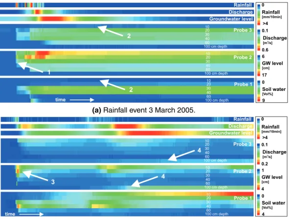
Three typical events are shown in Fig. 2. Probe 1 is located at the lower end and

probe 3 at the upper end of the hillslope transect. Details of event response and

an-tecedent conditions are listed in Table1.

For the first event, the event on March 3rd 2005 (Fig.2a), total precipitation amounted

to 52 mm with a highest intensity of 8.6 mm/10 min. The maximum change in soil

mois-10

ture was high with 8.6 Vol%, which is due to the fact that this event was the rainfall event with the lowest antecedent moisture content of all events studied. The most prominent patterns found for this event are a) extremely fast vertical water transport (arrow 1 in

Fig. 2a), due to high rainfall intensities and high hydraulic conductivities, and b) very

little reaction at the 10 cm depth for probes 1 and 3 (arrow 2 in Fig.2a). This is

prob-15

ably due to hydrophobicity resulting from the dry antecedent moisture conditions. This pattern was observed only for the 3 driest occasions. Soil moisture increase below the hydrophobic layer must be due to lateral inputs, either at the the decimeter scale or at the hillslope scale. Potential hydrophobicity of soil samples from 5 to 80 cm depth was tested with the Water Drop Penetration Time test. It was found that while the

20

top horizons show strong to extreme water repellency, samples from greater depths

are wettable (Table 2). However, this test determines only potential hydrophobicity,

measured in air dried soil. Water repellency under field conditions is likely to be less pronounced.

The rainfall event on April 6th 2005 (Fig.2b) has a total precipitation of 28 mm and

25

only low rainfall intensities. The maximum increase in soil moisture, as well as

stream-flow and groundwater levels are low with 3.8 Vol%, 0.06 m3/s and 3 cm, respectively

(Table1). The major patterns found here are: a) fast vertical water transport, due to

(13)

HESSD

4, 2587–2624, 2007

T. Blume et al.

Title Page

Tables Figures

◭ ◮

Back Close

Full Screen / Esc

EGU 100 cm depth for probes 2 and 3, while no such reaction can be seen at the 60 cm

sen-sor (arrow 4 in Fig.2b). As water is apparently not transported to this point vertically,

this seems to be the result of lateral water input, causing a slow trailing “wave” at this depth.

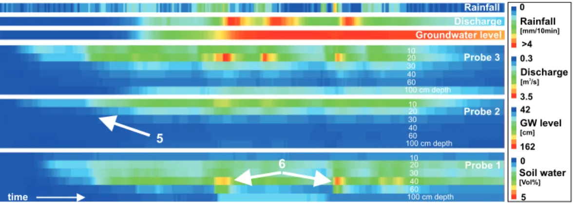
The event on 27 May 2005 (Fig.2c) has a very high total precipitation of 124 mm with

5

a highest intensity of 3.2 mm/10 min. However, as this event is probably a rain on snow

event, it is difficult to estimate the actual amount of water entering the soil. While the

response of discharge (3.22 m3/s increase), and ground water levels (120 cm increase)

is extremely strong, soil moisture shows a much less pronounced reaction. This is explained by the fact that this is not only an event with high rainfall amounts, but that

10

snow was also present in the catchment at this time (30 cm of snow were measured at the climate station just outside of the research catchment at 1270 m elevation, while the soil moisture transect is located at about 1140 m elevation.). Therefore some of the

runo_ffmight be generated at the snow surface or within the snow layer. Furthermore, as

all water in excess of field capacity is likely to be transported quickly to greater depths,

15

soil moisture increases most for dry antecedent conditions and less in conditions of high antecedent wetness, which was the case during this event. The most prominent patterns for this event are: a) slow vertical water transport, probably due to lower rainfall

intensities (arrow 5 in Fig.2c) and b) strong response at 40 cm depth for probe 1, very

local and short-term (arrow 6 in Fig.2c). This reaction might be due to an underlying

20

capillary barrier, causing the water to pond above it until breakthrough. This pattern was observed at this location quite frequently (for 15 events out of 34).

4.2 Dye tracer rainfall simulation

In May 2006 rainfall simulation experiments with blue dye were carried out at the loca-tions of the three continuously measuring probes. The soil moisture dynamics of these

25

three experiments are shown in Fig.3. As the same amount of dye was applied over

(14)

HESSD

4, 2587–2624, 2007

T. Blume et al.

Title Page

Tables Figures

◭ ◮

Back Close

Full Screen / Esc

time period and intensity of dye application is plotted in the top bar. The same colour

scale was applied for the intensity of application as for the rainfall intensities in Fig.2.

Neither streamflow nor groundwater level dynamics are plotted as there was no reac-tion to these small scale experiments (small in comparison to the size of the hillslope). The mean antecedent moisture content for the top 30 cm was 27.7 Vol%. The dynamic

5

moisture patterns show fast/preferential vertical flow for probes 1 and 2 and slow

ver-tical water transfer for probe 3 (Fig.3). One day after the beginning of the sprinkling

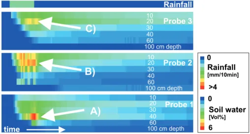
experiment, crossections of the infiltration plots were excavated and the dye stain pat-terns marking the flow paths of the dye in the unsaturated zone were photographed. The three photos of the crossections at the locations of the soil moisture probes are

10

shown in Fig.4. Preferential flow is found at all three plots. Flow occurred in plumes,

which are separated by distinct areas of little or no flow and thus are not marked by blue dye.

Figure 4a shows the flow paths of probe 1 (located at the bottom of the slope).

While blue dye can be seen in the top 5 cm, hardly any dye stains could be found in

15

depths of 5–ca. 30 cm (arrow 1 in Fig.4a). This is most likely the suspected zone of

hydrophobicity which was also found in the analysis of the time-space maps of soil moisture response to rainfall events. This zone of hydrophobicity or water repellency is most pronounced after summer dry periods but is still visible at the time of the sprinkling

experiment where only little reaction was seen at the 10 cm sensor of probe 1 (Fig.3).

20

Distinct plumes of dye can be found at depths of ca. 30–60 cm (arrow 2 in Fig.4a) (also

at the location of the soil moisture probe), just above a very pronounced layer interface

between the silty sand layer above and the gravelly layer below (arrow 3 in Fig.4a).

This confirms the hypothesis that a capillary barrier could be the cause of the ponding

at the 40 cm sensor which was seen in the event response analysis (Fig.3, arrow A).

25

The dye stains also indicated the locations were water leached into the capillary barrier

(arrow 3 in Fig.4a). The maximum depth of dye infiltration was about 1 m. Probe 1

(15)

HESSD

4, 2587–2624, 2007

T. Blume et al.

Title Page

Tables Figures

◭ ◮

Back Close

Full Screen / Esc

EGU the 10 cm and sometimes also the 20 cm sensor are surrounded by hydrophobic soil

(Figs.2a and b).

The crosssection at probe 2 (Fig. 4b) shows as most distinct feature the saprolite

layer (weathered bedrock) starting at the location of the 60 cm sensor (arrow 1 in

Fig. 4b). The 100 cm sensor is thus located within the saprolite. It was also found

5

that the probe is located within a preferential flow path coinciding with a concentration

of fine roots (arrow 2 in Fig.4b). Maximum infiltration depth is about 80 cm in the three

major plumes. A hydrophobic layer with very little staining can be seen in the

crossec-tion (arrow 1 in Fig. 4b). However, this layer was not identified in the soil moisture

data, as the probe is located within the preferential flow path and not in a hydrophobic

10

patch. The high velocity of flow and the strong response in this preferential flow path

is also visible in Fig.3(arrow B) and was also a feature of the soil moisture response

space-time maps at this location.

The soil at probe 3 (Fig.4c) differed compared to the two others as the vegetation

at this plot included a thicket of low shrubs, causing a higher density of roots in the

15

top 20 cm (arrow 1 in Fig. 4c). The probe was here located in between dye stained

preferential flow paths. While blue dye is found in the vicinity of the probe at depths 10– 20 cm, very little of it is found close to the probe at greater depths. The 60 cm sensor is located just at the interface between the silty sand and layer of fine gravel (arrow 2

in Fig.4c), thus probably measuring in both layers, while the 100 cm sensor is situated

20

in a layer of more compacted silty sand starting at a depth of approx. 75 cm. Maximum depth of infiltration is 80 cm. The fact that the layer at the 100 cm sensor is more compacted might explain why reaction at this sensor occurs delayed and prolonged. This would correspond to lower hydraulic conductivities in the compacted layer causing a delay in response and a prolonged peak. However, as the response at the 60 cm

25

sensor is often very weak, the water causing the peak at 100 cm depths is most likely transported to this point not vertically but laterally. The dense root zone in the top 20 cm

explains the strong reaction at the 20 cm sensor (Fig.3, arrow C). Probe 3 shows a

(16)

HESSD

4, 2587–2624, 2007

T. Blume et al.

Title Page

Tables Figures

◭ ◮

Back Close

Full Screen / Esc

which is explained by the fact that this probe is not situated within a preferential flow path.

4.3 Response times

A comparison of response lags for 27 rainfall events between December 2004 and

April 2006 is shown in Fig.5. S20, S30, S40 are the response lags of the soil moisture

5

sensors at 20, 30 and 40 cm depth, GW is the response lag of ground water level

at well W1 (Fig. 1) and Q is the response lag of stream flow. Response lags of all

parameters show similar behavior over time: response times are short from January to April (summer and early fall) when compared to the winter months. This is probably the result of a) enhanced preferential flow due to hydrophobicity and b) higher rainfall

10

intensities. Groundwater response is generally slower than stream flow response. (At this hillslope the groundwater surface at well W1 in the vicinity of the stream is generally about 60 cm below the stream bed.) Surprisingly, the soil moisture sensors often react slower than stream flow. This could either mean that rainfall is not uniformly distributed over the catchment or that these sensors are bypassed by preferential flow paths.

15

Surface runoffis unlikely, due to high infiltration rates and porosities and has not been

observed during field campaigns.

4.4 Annual dynamics of soil moisture

The annual dynamics of soil moisture, in Fig. 6 shown exemplary for probe 3

(Octo-ber 2004–May 2006), are little pronounced in comparison to the event dynamics. Only

20

during the summer months (January and February) a short drying period can be

ob-served (circled in Fig.6). However, as soon as the first rainfalls start in autumn, soil

moisture values rebound to their previous level. The fact that soil moisture values for the 20 cm depth are high compared to the 10 and 30 cm depths is either due to textural

di_fferences or to a root found close to this sensor during the excavation of this profile

25

(17)

HESSD

4, 2587–2624, 2007

T. Blume et al.

Title Page

Tables Figures

◭ ◮

Back Close

Full Screen / Esc

EGU

4.5 Soil moisture spatial patterns at the hillslope scale

Soil moisture patterns at the two transects are depicted in Fig.7. It was found that

patterns are quite persistent over time. There seems to be a correlation with position on the slope for the 10 cm sensor, but not for the sensors at greater depths. At 10 cm depth the lower part of the slope is generally wetter than the upper part of the slope.

5

This is probably due to shading effects: the deeper in the steep valley the fewer hours

of direct sunshine. The northern transect is wetter than the southern transect, which is probably due to denser vegetation.

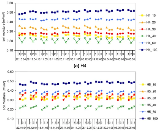
4.6 Variability of soil moisture at the decimeter scale

Profile probes measure predominantly in a certain direction. By taking three

mea-10

surements, turning the probe by 120◦ each time, the full circle is covered. Figure 8

shows the small scale variability in soil moisture measured by twisting the probes at

the manual measurement points H4 and H5. Differences in soil moisture around the

probe can be very pronounced, e.g. it is wetter/drier in one direction than in the others. These patterns of small scale variability are quite persistent over time while the

tem-15

poral variability of soil moisture at this time resolution (irregular time intervals during field campaigns) is generally low. It can be seen that while for measurement point H4 only the 20 and the 40 cm sensor show a stronger directional variability of 2.3 Vol% and 4.3 Vol%, respectively, this phenomenon is found for all depths but the 100 cm level at location H5. Overall 68% of the sensors show directional variability (median

20

variability≥1.8 Vol%) when counting each sensor along the probes separately (i.e. 6

depths times 11 locations). 29% of all sensors have a variability≥3 Vol%, 18% have

a variability ≥4 Vol% and 6% show a variability of more than 5 Vol%. As the profile

probes have a range of only 10 cm, this observed variability of soil moisture occurs on a very small scale, the scale of decimeters. A possible explanation for these strong

25

gradients in water content over such a small distance is the presence of preferential

(18)

HESSD

4, 2587–2624, 2007

T. Blume et al.

Title Page

Tables Figures

◭ ◮

Back Close

Full Screen / Esc

as during a more extended dye tracer study in this catchment (Blume et al., 2007b2).

If a sensor is located near the interface of such a preferential flow path, soil moisture

will di_ffer considerably depending on the direction of the measurement. The scale or

width of these flow paths is in the order of <3 decimeters, thus matching the scale

of the measurement. A sensor showing no directional variation must therefore be

lo-5

cated either in the center of a flow path or in the center of the matrix with no flow path

within reach of the measurement. Ritsema and Dekker(1996) also used small scale

(5–10 cm) variability of soil moisture as a measure for preferential or finger flow. In their study moisture gradients between flow paths and non-flow areas ranged between 3 and 6 Vol%. Assuming small scale soil moisture variability does indeed indicate the

10

presence of a preferential flow path, the fact that in Malalcahuello 68% of all sensors show this type of variability also gives us a measure of the importance of preferential flow in this catchment. There are five possible explanations for the surprising persis-tency of these soil moisture patterns (or preferential flow patterns) over the course of

more than one and a half years (Fig.8).

15

1. These patterns might be caused by air gaps between access tube and the sur-rounding soil due to faulty installation. However, special care was taken to avoid this problem, by using the auger supplied by the manufacturer of the probes. Fur-thermore no noticeable air gaps were found during excavation of the probes at the end of the field study, on the contrary, probes were sitting tightly in the soil.

20

2. They might also be due to textural differences. However, as the sensors have only

a range of 10 cm the measured volume is likely to be located within a single layer.

3. These patterns might also be induced by roots, which are not likely to change po-sition on this time scale. However, roots were only found in some instances were these preferential flow patterns were observed during dye tracer experiments.

25 2

(19)

HESSD

4, 2587–2624, 2007

T. Blume et al.

Title Page

Tables Figures

◭ ◮

Back Close

Full Screen / Esc

EGU 4. They might be due to hydrophobicity in some parts of the soil, which would

pro-duce self reinforcing patterns likely to persist if not subjected to long periods of saturation.

5. These patterns could also be self reinforcing due to the strong gradient in soil moisture itself, leading to faster vertical transport within the wetter area (the flow

5

path) than lateral flow into the drier area as a result of the strong gradient in matric potential.

This last possibility was investigated by calculating the unsaturated conductivities for a number of gradients in soil moisture and thus matric potential: from 20 to 25 Vol%, from 25 to 30 Vol% and from 30 to 35 Vol%, thus covering the range from 20 to 35 Vol%

10

of soil moisture, where most of the variability was observed. The gradient of 5 Vol% chosen to investigate this phenomenon was in the upper range of gradients observed in the field (as the profile probes are not measuring unilaterally in one direction, the gradients perpendicular to a flow path interface are likely to be even higher than the gradients obtained from these measurements). In order to compare flow within the

15

flow path with flow perpendicular to the flow path interface a three step calculation was carried out: First, the Van Genuchten parameters were obtained through fitting the Van Genuchten equation to the soil moisture characteristic curves. Then the gradient in matric potential was determined for the above gradients in soil moisture from the soil moisture characteristic curves. The Van Genuchten equation can then be used to

20

determine the unsaturated conductivities for the chosen matric potential. As the longi-tudinal distance a length of 10 cm was chosen, as this is the range of the instrument. The ratio of the gradients in potential (across interface/within flow path) was then com-pared with the ratio of the unsaturated hydraulic conductivities (within the flow path/

across the interface). The effective unsaturated hydraulic conductivity across the flow

25

path interface was calculated by treating the interface as two layers of differing

conduc-tivity (due to the di_fferences in water content) and therefore using the harmonic mean

(20)

HESSD

4, 2587–2624, 2007

T. Blume et al.

Title Page

Tables Figures

◭ ◮

Back Close

Full Screen / Esc

to 1 [cm H₂O/cm]. In case the ratio of the of the unsaturated hydraulic conductivities

is much larger than the gradient in matric potential across the interface (Eq.1), these

flow paths are likely to persist over time.

K_θ(flow path)

m/s

K_θ(interface)

m/s ≫

∆ψ(interface)

cm H₂O/cm

1

cm H2O/cm

(1)

It was found that this would indeed be the case for a pure sand (with a ratio ofKθup

5

to 11 times larger than the ratio of∆ψ), however, in these soils, which have a fraction

of at least 20% silt, it is very difficult to achieve these conditions (the ratio of K_θ is

less than half that of the ratio of _∆ψ). It is thus unlikely that solely the gradient in

soil moisture causes the flow paths to persist in time. Nevertheless, if the unsaturated

conductivity across the interface is further diminished by the effects of hydrophobicity

10

a persistant pattern becomes more probable. Furthermore this type of soil is known to

be hysteretic (Shoji et al.,1993;Musiake et al.,1988) thus causing a shift in the wetting

curve compared to the here used draining curve, which could also change the outcome of this rough estimation. Persistent fingers as a result of hysteresis of the soil moisture

characteristic curves were described bySelker et al.(1996) andNieber(1996).Nieber

15

(1996) explains that fingers will persist if the water entry pressure on the main wetting

curve is smaller then the air entry pressure on the main drainage curve. However, due

to lack of information on the main wetting curve, this effect cannot be assessed for the

soils in the Malalcahuello Catchment.

5 Conclusions

20

The soil moisture data obtained in this study provided diverse insights covering diff

er-ent aspects of runoffgeneration processes in this catchment. It was shown that high

(21)

HESSD

4, 2587–2624, 2007

T. Blume et al.

Title Page

Tables Figures

◭ ◮

Back Close

Full Screen / Esc

EGU

investigating runoffgeneration processes. This is especially true for catchments where

only short time series of data are available, as in the Malalcahuello Catchment. The approach of combining high temporal but spatially scarce data with episodic additional measurements allowed for the investigation of soil moisture dynamics as well as pat-terns and proved to be less expensive than high density installation of continuously

5

logging sensors while also being applicable to difficult terrain, i.e. densely forested and

steep hillslopes.

By analyzing the dynamics of soil moisture response to rainfall events with the help of space-time maps it was possible to identify a number of patterns which can be

attributed to different phenomena of flow in the unsaturated zone. The very subdued

10

response of soil moisture in the upper soil horizon at two locations during the driest period (late summer) was attributed to the formation or reinforcement of hydrophobicity in this layer. The accumulation/ponding of water at certain depths was assumed to be

due to the e_ffect of capillary barriers. This was confirmed by the dye tracer experiment

carried out at this location. Strong response at certain depths while the layers just

15

above show little reaction indicate the importance of lateral flow processes.

It was furthermore found that infiltration dynamics differed from summer to winter,

which could be due to differences in rainfall intensities as well as the amplification of

preferential flow due to hydrophobicity in the top layer. Potential water repellency was

tested with “Water Drop Penetration Time”-method (e.g. Dekker and Ritsema,1994)

20

and was found to be strong to extreme for the upper horizon. Hydrophobicity has been

observed in these Chilean young volcanic ash soils by other researchers (Bachmann

et al., 2000; Ellies,1975) and is also of importance in volcanic ash soils of Ecuador

(Poulenard et al.,2004). Differences in flow patterns from dry to wet period were also found in the Malalcahuello Catchment during a more extensive study involving a total

25

of 10 dye tracer experiments (Blume et al., 2007b2). The change in flow pattern

ob-served in this study further supports the theory that preferential flow in this catchment is reinforced by hydrophobicity. Similar flow patterns also attributed to hydrophobicity

(22)

Rit-HESSD

4, 2587–2624, 2007

T. Blume et al.

Title Page

Tables Figures

◭ ◮

Back Close

Full Screen / Esc

sema and Dekker,1994;Dekker and Ritsema,2000;de Rooij, 2000). The fact that

throughfall amounts are highly heterogenous in this catchment (Blume et al., 2007a1)

is likely to be the reason why some locations (probably on the decimeter scale) are drier than others and thus more likely to develop water repellency. Spots of high water input are therefore likely to become preferential flow paths. These observed patterns

5

in dynamics were found to be spatially and temporally persistent insofar as the event

pattern dynamics of soil moisture observed in Fall 2005 (Fig.2) matched well with the

flow patterns found during the dye tracer experiments one year later. The persistency

of the spatial patterns of soil moisture for 14 locations and 6 depths (Fig.7) shows that

spatial variability is much higher than temporal variability and that wetter locations are

10

likely to remain wet. Furthermore the patterns of soil moisture variability at the decime-ter scale, which were also attributed to the presence/absence of preferential flow paths, were found to be persistent over a period of more than one and a half years. While in

the case of the larger scale soil moisture patterns the spatial di_fferences in water

con-tent could also be attributed to differences in soil texture, the small scale variability is

15

most likely located within a single soil layer and thus not caused by textural differences.

Other possible causes for the observed flow patterns/finger flow apart from hy-drophobicity are: flow along roots or preferential flow paths maintained purely by the strong gradient in soil moisture and thus also in unsaturated conductivity. However, roots were found only in some cases of preferential flow patterns. Furthermore, a

20

simple back-of-the-envelope calculation of unsaturated conductivities within and in be-tween flow paths and their corresponding gradients in matric potential showed that these flow paths might be self-reinforcing in pure sand but not in this type of soil. Hy-drophobicity is therefore still the most likely explanation for the flow patterns found here.

However, the effects of hydrophobicity are likely to be aggravated by root channels,

25

strong gradients in matric potential and the hysteresis of the soil moisture

characteris-tic curves of volcanic ash soils as described byShoji et al.(1993).

The last and maybe the most important question is the question of how important

(23)

re-HESSD

4, 2587–2624, 2007

T. Blume et al.

Title Page

Tables Figures

◭ ◮

Back Close

Full Screen / Esc

EGU

sponse/runoffgeneration at the catchment scale. Several findings indicate that while

preferential flow was only observed at the plot scale it might indeed be important factor

of runoffgeneration at the catchment scale. That preferential flow occurs throughout

the catchment is indicated by the fact that additionally to the three tracer experiments shown in this study all 9 dye tracer experiments carried out under forest at various

lo-5

cations in the catchment showed preferential flow patterns (Blume et al., 2007b2). The

fact that 68% of the sensors at the 11 manual measurement points showed small scale soil moisture variability is another indicator for the importance of these preferential flow paths. Last but not least the analysis of response times for soil moisture, groundwa-ter and streamflow reveiled that response lags are generally much shorgroundwa-ter during the

10

summer months were preferential flow is also likely to be further enforced by stronger hydrophobicity. Interestingly streamflow often shows faster response than both ground-water and soil ground-water. This might be due to non-uniform rainfall distribution (i.e. earlier onset of rainfall further up in the catchment causing stream levels to respond while soil moisture at the slope close to the catchment outlet remained unchanged). However, as

15

our data points in space are restricted to only three locations it is also likely that there are other preferential flow paths with even faster response than the ones measured by our instruments. In this case preferential flow in the vertical and then a fast reaction along a horizontal layer interface might be the reason for the short response lags of streamflow found in this catchment. (Finger flow is known to cause faster breakthrough

20

as investigated by de Rooij and deVries (1996) in a modelling study.) The question

whether or not these preferential flow processes are important for catchment response could be investigated further by application of a physically based hydrological model either on the hillslope or on the catchment scale.

To summarize the main conclusions in short:

25

1. the combination of high temporal resolution but spatially scarce soil moisture data with episodic additional measurements proved to be useful for the investigation

of runoffgeneration processes, especially with respect to preferential flow. While

(24)

num-HESSD

4, 2587–2624, 2007

T. Blume et al.

Title Page

Tables Figures

◭ ◮

Back Close

Full Screen / Esc

ber of continuously logging probes it is also suitable for difficult terrain (i.e. very

steep slopes) where geophysical techniques are problematic. The use of contin-uously monitored rainfall experiments with subsequent excavation of soil profiles adds additional insights into the flow processes in the unsaturated zone.

2. soil moisture/flow patterns were shown to be persistent in time and highly variable

5

in space

3. the most likely explanation for the observed flow patterns is a combination of hy-drophobicity with strong gradients in unsaturated conductivities, were flow paths are caused either by the presence of roots or the highly heterogeneous distribu-tion of throughfall and thus water input

10

4. the flow patterns observed at the local scale are likely to be important for runoff

response at the catchment scale.

Acknowledgements. The authors would like to thank A. Bauer, D. Reusser (Potsdam Univer-sity) and H. Palacios, L. Opazo (Universidad Austral de Chile) for help in the field, and A. Iroum ´e and A. Huber (Universidad Austral de Chile) for logistic and technical assistance. This work

15

was partially funded by the International Office of the BMBF (German Ministry for Education and Research) and Conicyt (Comisi ón Nacional de Investigaci ón Cient´ıfica y Tecnol ógica de Chile) and the “Potsdam Graduate School of Earth Surface Processes”, funded by the State of Brandenburg.

References

20

Bachmann, J., Ellies, A., and Hartge, K. H.: Development and application of a new sessile drop contact angle method to assess soil water repellency, J. Hydrol., 231, 66–75, 2000.2607

Bardossy, A. and Lehmann, W.: Spatial distribution of soil moisture in a small catchment. Part 1: Geostatistical analysis, J. Hydrol., 206, 1–15, 1998.2590

Blume, T., Zehe, E., and Bronstert, A.: Rainfall runoffresponse, event-based runoffcoefficients

25

(25)

HESSD

4, 2587–2624, 2007

T. Blume et al.

Title Page

Tables Figures

◭ ◮

Back Close

Full Screen / Esc

EGU

Brocca, L., Morbidelli, R., Melone, F., and Moramarco, T.: Soil moisture spatial variability in experimental areas of central Italy, J. Hydrol., 333, 356–373, 2007.2590

de Rooij, G. H.: Modeling fingered flow of water in soils owing to wetting front instability: a review, J. Hydrol., 231, 277–294, 2000. 2608

de Rooij, G. H. and deVries, P.: Solute leaching in a sandy soil with a water-repellent surface

5

layer: A simulation, Geoderma, 70, 253–263, 1996. 2609

Dekker, L. W. and Ritsema, C. J.: How Water Moves in a Water Repellent Sandy Soil .1. Potential and Actual Water Repellency, Water Resour. Res., 30, 2507–2517, 1994. 2597,

2607

Dekker, L. W. and Ritsema, C. J.: Wetting patterns and moisture variability in water repellent

10

Dutch soils, J. Hydrol., 231, 148–164, 2000. 2608

Ellies, A.: Untersuchungen über einige Aspekte des Wasserhaushaltes vulkanischer As-chenb öden aus der gem äßigten Zone S üdchiles, PhD thesis, Technical University of Han-nover, Germany, HanHan-nover, 1975. 2607

Frisbee, M., Allan, C., Thomasson, M., and Mackereth, R.: Hillslope hydrology and wetland

15

response of two small zero-order boreal catchments on the Precambrian Shield, Hydrol. Process., early view, doi:10.1002/hyp.6521, 2007. 2590

Germann, P. F. and Zimmermann, M.: Water balance approach to the in situ estimation of volume flux densities using slanted TDR wave guides, Soil Sci., 170, 3–12, 2005. 2590

Hasegawa, S.: Evaluation of rainfall infiltration characteristics in a volcanic ash soil by time

20

domain reflectometry method, Hydrol. Earth Syst. Sci., 1, 303–312, 1997,

http://www.hydrol-earth-syst-sci.net/1/303/1997/. 2589

Hino, M., Odaka, Y., Nadaoka, K., and Sato, A.: Effect of Initial Soil-Moisture Content on the Vertical Infiltration Process – a Guide to the Problem of Runoff-Ratio and Loss, J. Hydrol., 102, 267–284, 1988. 2590

25

Iroum ´e, A.: Transporte de sedimentos en una cuenca de montana en la Cordillera de los Andes de la Novena Region de Chile, Bosque, 24, 125–135, 2003.2592

Kienzler, P. and Naef, F.: Subsurface storm flow formation at di_fferent hillslopes and implications fro the ‘old water paradox’, Hydrol. Process., early view, doi:10.1002/hyp.6687, 2007. 2590

McNamara, J. P., Chandler, D., Seyfried, M., and Achet, S.: Soil moisture states, lateral flow,

30

and streamflow generation in a semi-arid, snowmelt-driven catchment, Hydrol. Process., 19, 4023–4038, 2005. 2590

(26)

HESSD

4, 2587–2624, 2007

T. Blume et al.

Title Page

Tables Figures

◭ ◮

Back Close

Full Screen / Esc

patterns in a small Dartmoor catchment, Southwest England, Hydrol. Process., 17, 251–264, 2003. 2590

Musiake, K., Oka, Y., and Koike, M.: Unsaturated Zone Soil-Moisture Behavior under Temper-ate Humid Climatic Conditions – Tensiometric Observations and Numerical Simulations, J. Hydrol., 102, 179–200, 1988.2589,2606

5

Nieber, J. L.: Modeling finger development and persistence in initially dry porous media, Geo-derma, 70, 207–229, 1996. 2606

Nyberg, L.: Spatial variability of soil water content in the covered catchment at Gardsjon, Swe-den., Hydrol. Process., 10, 89–103, 1996.2590

Poulenard, J., Michel, J. C., Bartoli, F., Portal, J. M., and Podwojewski, P.: Water repellency

10

of volcanic ash soils from Ecuadorian paramo: effect of water content and characteristics of hydrophobic organic matter, Eur. J. Soil Sci., 55, 487–496, 2004. 2607

Rezzoug, A., Schumann, A., Chi_fflard, P., and Zepp, H.: Field measurement of soil moisture dynamics and numerical simulation using the kinematic wave approximation, Adv. Water Resour., 28, 917–926, 2005.2590

15

Ritsema, C. J. and Dekker, L. W.: How Water Moves in a Water Repellent Sandy Soil .2. Dynamics of Fingered Flow, Water Resour. Res., 30, 2519–2531, 1994.2607

Ritsema, C. J. and Dekker, L. W.: Water repellency and its role in forming preferred flow paths in soils, Aust. J. Soil Res., 34, 475–487, 1996.2604

Ritsema, C. J. and Dekker, L. W.: Preferential flow in water repellent sandy soils: principles and

20

modeling implications, J. Hydrol., 231, 308–319, 2000. 2607

Ritsema, C. J., Dekker, L. W., Nieber, J. L., and Steenhuis, T. S.: Modeling and field evidence of finger formation and finger recurrence in a water repellent sandy soil, Water Resour. Res., 34, 555–567, 1998.2607

Selker, J. S., Steenhuis, T. S., and Parlange, J. Y.: An engineering approach to fingered vadose

25

pollutant transport, Geoderma, 70, 197–206, 1996. 2606

Shoji, S., Nanzyo, M., and Dahlgren, R.: Volcanic ash soils – genesis, properties and utilization, in: Developments in soil science, vol. 21, Elsevier, Amsterdam, 1993. 2606,2608

Starr, J. L. and Timlin, D. J.: Using high-resolution soil moisture data to assess soil water dynamics in the vadose zone, Vadose Zone J., 3, 926–935, 2004. 2590

30

Taumer, K., Stoffregen, H., and Wessolek, G.: Seasonal dynamics of preferential flow in a water repellent soil, Vadose Zone J., 5, 405–411, 2006. 2590

(27)

HESSD

4, 2587–2624, 2007

T. Blume et al.

Title Page

Tables Figures

◭ ◮

Back Close

Full Screen / Esc

EGU

Zealand, Eos T. Am. Geophys. Un., 35, 136–144, 1954. 2589

Weiler, M. and Naef, F.: An experimental tracer study of the role of macropores in infiltration in grassland soils, Hydrol. Process., 17, 477–493, 2003. 2591,2596

Western, A. W., Zhou, S.-L., Grayson, R. B., McMahon, S. D., Bloschl, G., and Wilson, D. J.: Spatial correlation of soil moisture in small catchments and its relationship to dominant

spa-5

tial hydrological processes, J. Hydrol., 286, 113–134, 2004. 2590

Williams, A. G., Dowd, J. F., Scholefield, D., Holden, N. M., and Deeks, L. K.: Preferential flow variability in a well-structured soil, Soil Sci. Soc. Am. J., 67, 1272–1281, 2003. 2590

Zhou, Q. Y., Shimada, J., and Sato, A.: Three-dimensional spatial and temporal monitoring of soil water content using electrical resistivity tomography, Water Resour. Res., 37, 273–285,

10

2001. 2590

(28)

HESSD

4, 2587–2624, 2007

T. Blume et al.

Title Page

Tables Figures

◭ ◮

Back Close

Full Screen / Esc

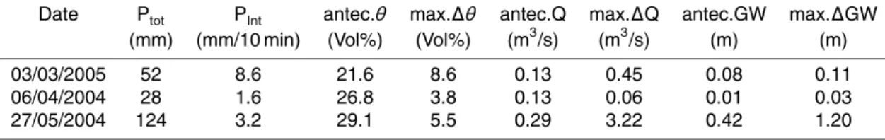
Table 1. Response characteristics and antecedent conditions for the three events shown in

Fig.2 (P_tot = rainfall amount, P_Int = maximum rainfall intensity, antec.θ =antecedent mean soil moisture content for the top 30 cm, max.∆θ =max. increase in soil moisture of all sen-sors, antec.Q=antecedent streamflow, max.∆Q=max. increase in streamflow, antec.GW=

antecedent groundwater level at well W1, max.∆GW=max. increase in groundwater levels).

Date P_tot P_Int antec.θ max.∆θ antec.Q max.∆Q antec.GW max.∆GW (mm) (mm/10 min) (Vol%) (Vol%) (m3/s) (m3/s) (m) (m)

(29)

HESSD

4, 2587–2624, 2007

T. Blume et al.

Title Page

Tables Figures

◭ ◮

Back Close

Full Screen / Esc

EGU

Table 2. Results of the Water Drop Penetration Time (WDPT) test. If a sample showed water

repellency the WDPT test was carried out with 12 repetitions, i.e. with 12 sub-samples. Shown are the number of tests per sample falling in the different classes of water repellency. Samples “forest 1-3” were taken at the slope of the soil moisture transect, while samples named “pine” were taken in a pine plantation downstream of the catchment outlet.

location depth wettable slightly strongly severely extremely (cm) water repellent water repellent water repellent water repellent

forest 1 5–10 no – – 5 7

forest 1 10–15 no – 2 3 7 forest 2 10–20 no – 12 – – forest 2 20–60 yes – – – – forest 2 60–80 yes – – – – forest 3 10–20 no 3 9 – – forest 3 20–60 yes – – – – forest 3 60–80 yes – – – –

pine 0–5 no – – – 12

pine 5–20 no 12 – – –

pine 20–60 yes – – – –

(30)

HESSD

4, 2587–2624, 2007

T. Blume et al.

Title Page

Tables Figures

◭ ◮

Back Close

Full Screen / Esc

✁

✂✄

☎✆

✝✞

✟✠

✡

☛

☞✌

rain gauge

✍

✎

stream gauge

0 500 1000 1500 Meters

✏✑✓✒

✔

✕

✖✘✗

✙

✚✜✛ ✢✤✣✦✥★✧

✩✫✪

✬✮✭✯

✰

1120

12₀₀

✱✲

stream gauge

✳

observation well

✴

soil moisture (manual)

✵

soil moisture (cont.) catchment boundary

rain gauge 50 m downstream

P1 P2

P3

W1 0 10 20 Meters

Fig. 1. Left: The Malalcahuello Catchment including the positions of rain gauges and the

(31)

HESSD

4, 2587–2624, 2007

T. Blume et al.

Title Page Abstract Introduction Conclusions References Tables Figures ◭ ◮ ◭ ◮ Back Close

Full Screen / Esc

Printer-friendly Version Interactive Discussion EGU Rainfall Discharge Groundwater level Probe 3 Probe 2 Probe 1 10 20 30 40 60 100 cm depth

Rainfall

[mm/10min]

GW level

[cm]

Discharge

[m /s]3

Soil water [Vol%] 0 >4 6 17 0.1 0.6 0 9 10 20 30 40 60 100 cm depth 10 20 30 40 60 100 cm depth

time

1

2 2

(a)Rainfall event 3 March 2005.

Rainfall Discharge Groundwater level Probe 3 Probe 2 Probe 1 10 20 30 40 60 100 cm depth