www.hydrol-earth-syst-sci.net/13/1215/2009/ © Author(s) 2009. This work is distributed under the Creative Commons Attribution 3.0 License.
Earth System
Sciences
Use of soil moisture dynamics and patterns at different
spatio-temporal scales for the investigation of subsurface flow
processes
T. Blume1,2,*, E. Zehe3, and A. Bronstert1
1Institute for Geoecology, Section of Hydrology and Climatology, University of Potsdam, Germany 2Helmholtz Centre Potsdam, GFZ German Research Centre for Geosciences, Germany
3Institute for Water and Environment, Technical University Munich, Germany
*Invited contribution by T. Blume, one of the EGU Young Scientists’ Outstanding Poster Paper (YSOPP) Award winners 2008.
Received: 3 August 2007 – Published in Hydrol. Earth Syst. Sci. Discuss.: 9 August 2007 Revised: 2 June 2009 – Accepted: 29 June 2009 – Published: 17 July 2009
Abstract. Spatial patterns as well as temporal dynamics of soil moisture have a major influence on runoff genera-tion. The investigation of these dynamics and patterns can thus yield valuable information on hydrological processes, especially in data scarce or previously ungauged catchments. The combination of spatially scarce but temporally high res-olution soil moisture profiles with episodic and thus tem-porally scarce moisture profiles at additional locations pro-vides information on spatial as well as temporal patterns of soil moisture at the hillslope transect scale. This ap-proach is better suited to difficult terrain (dense forest, steep slopes) than geophysical techniques and at the same time less cost-intensive than a high resolution grid of continu-ously measuring sensors. Rainfall simulation experiments with dye tracers while continuously monitoring soil moisture response allows for visualization of flow processes in the un-saturated zone at these locations. Data was analyzed at differ-ent spacio-temporal scales using various graphical methods, such as space-time colour maps (for the event and plot scale) and binary indicator maps (for the long-term and hillslope scale). Annual dynamics of soil moisture and decimeter-scale variability were also investigated. The proposed ap-proach proved to be successful in the investigation of flow processes in the unsaturated zone and showed the importance of preferential flow in the Malalcahuello Catchment, a data-scarce catchment in the Andes of Southern Chile. Fast re-sponse times of stream flow indicate that preferential flow
Correspondence to:T. Blume ([email protected])
observed at the plot scale might also be of importance at the hillslope or catchment scale. Flow patterns were highly vari-able in space but persistent in time. The most likely explana-tion for preferential flow in this catchment is a combinaexplana-tion of hydrophobicity, small scale heterogeneity in rainfall due to redistribution in the canopy and strong gradients in unsat-urated conductivities leading to self-reinforcing flow paths.
1 Introduction
Identification of patterns of soil moisture response to rainfall and especially the vertical dynamics of soil moisture at the hillslope or plot scale can be useful for the investigation of runoff generation processes in previously ungauged or data scarce catchments (runoff generation is here referring to all components of streamflow: groundwater, subsurface storm-flow and surface runoff). When investigating runoff gener-ation processes in a previously ungauged catchment it be-comes obvious from the start that the equipment we are about to install is insufficient. There will be neither enough data points in time nor in space to characterize these processes in their temporal and spatial variability. A possible way to overcome this problem is the approach where a multitude of experimental methods is applied within a relatively short time frame, producing a data set that highlights a multitude of angles and aspects of catchment functioning. This type of study was carried out in the Malalcahuello Catchment in the Chilean Andes and is described in Blume et al. (2008a).
resolution soil moisture dynamics were found in our litera-ture search. However, in other parts of the world such as New Zealand or Japan the soil moisture dynamics of volcanic ash soils has been investigated to some extent: Hasegawa (1997) used hourly TDR data to investigate soil water con-ditions and movement, Eguchi and Hasegawa (2008) used TDR and tensiometer data to estimate preferential flow, Mu-siake et al. (1988) used tensiometric observations and a nu-merical model to study infiltration and drying behaviour of these soils and Van’t Woudt (1954) used 19 small lysimeters to investigate subsurface stormflow.
Soil moisture data has been used as a means to understand runoff generation in other parts of the world (e.g. Kienzler and Naef, 2007; Meyles et al., 2003; McNamara et al., 2005; Frisbee et al., 2007; Germann and Zimmermann, 2005; Zhou et al., 2002; Hino et al., 1988) or for the investigation of the effects of changes in land use or management on hydrologi-cal processes (Williams et al., 2003; Starr and Timlin, 2004). See also Robinson et al. (2008) and Vereecken et al. (2008) for comprehensive reviews on measurement techniques and the value of soil moisture data, respectively. In most stud-ies soil moisture was measured either with high spatial or with high temporal resolution, thus producing either spatial soil moisture patterns (Bardossy and Lehmann, 1998; Brocca et al., 2007; Meyles et al., 2003; Williams et al., 2003; West-ern et al., 2004; Rezzoug et al., 2005; Nyberg, 1996) or infor-mation on the dynamics (e.g. McNamara et al., 2005; Starr and Timlin, 2004; Frisbee et al., 2007). A combination of both can only be achieved with either a large number of probes measuring continuously such as in Starr and Timlin (2004) and Taumer et al. (2006) or with geophysical methods such as described for example in Zhou et al. (2001), were electric resistivity tomography was used to investigate soil moisture dynamics on a 3.5×3.5 m plot at hourly resolution. However, the first of these two options is cost-intensive while the second is predominantly carried out on grassland, fields or bare soils with little topography and is not feasible in com-plex terrain. Furthermore, as no general petrophysical rela-tion to derive soil moisture from specific resistivity values is available, careful inversion and site specific calibration is needed. Combining data sets with different spatio-temporal resolution thus might be a viable cost-efficient alternative for difficult terrain. A recent study using a similar approach has been carried out in a small catchment in Australia, where 500 datapoints sampled on a weekly basis for 4 weeks were combined with 7 continuously measuring stations (Martinez et al., 2008).
At the Malalcahuello Catchment soil moisture was mea-sured on two steep hillslope transects. Data was collected with a data logger at high temporal resolution at three points and manually at irregular intervals at 11 additional points. Each measurement produces soil moisture data for 6 differ-ent depths along a vertical profile. While this is still a very small number of data points it is nevertheless possible to get a general understanding of the major processes
occur-ring within the unsaturated zone of this catchment. Data was analyzed using various graphical methods allowing for data exploration at different spatio-temporal scales. By carrying out rainfall simulation experiments using a dye tracer over each of the continuously measuring probes it was possible to corroborate our perception of flow in the unsaturated zone at these locations. This combination of high temporal resolu-tion soil moisture measurements, rainfall simularesolu-tion experi-ments and the use of dye tracers to reassess the conclusions gained from the soil moisture time series is noteworthy and has a high potential for synergetic effects. However, only one other study (Weiler and Naef, 2003) using a similar ap-proach but a slightly different layout was found in our lit-erature search. The study at the Malalcahuello catchment furthermore included the analysis of response times at the event scale, yearly soil moisture dynamics, spatial patterns and their long-term dynamics for 14 locations and 6 depths and the investigation of small scale soil moisture variability at the decimeter scale.
The four main questions of the study in the Malalcahuello Catchment were:
1. Can soil moisture data be used to investigate the dy-namic patterns of unsaturated flow?
2. Can novel ways of data-visualization (e.g. space time colour maps) give a better picture of subsurface flow processes than traditional line plots alone?
3. Can the combination of data sets with different spatio-temporal resolution have synergetic effects and thus yield additional insights?
4. Can the observed soil moisture patterns and dynamics be connected with entire system/catchment response?
2 Research area
2.1 The Malalcahuello catchment
The research area is situated in the Reserva Forestal Malalc-ahuello, in the Precordillera of the Andes, IX. Region, Chile. The catchment is located on the southern slope of Volc´an Lonquimay (38◦25.5′–38◦27′S; 71◦32.5′–71◦35′E).
Table 1. Soil physical characteristics for major horizons of the Trumao soils in the Malalcahuello Catchment. (Ksat-saturated hydraulic
conductivity, GSD-grain size distribution, FC-field capacity, PWP-permanent wilting point, n.d.-not determined. Values are median values unless otherwise stated.)
humus horizon 1 horizon 2 horizon 3 gravel pumice
color dark dark brown yellow brown reddish brown gray orange
occurrence common common common less common common less common
depth range (cm) upper limit 0 5–10 20–60 25–90 30–600 60
lower limit 5–10 20–60 60–130 45–170 50–710 90
Ksat(m/s) min 2.2E–04 7.0E–05 3.8E–05 2.0E–05 1.3E–03 1.0E–03
max 2.7E–03 8.2E–04 8.9E–04 6.1E–03 1.8E–03 2.8E–03
median 2.1E–03 2.6E–04 2.2E–04 9.6E–05 1.7E–03 2.2E–03
No.of samples 3 14 9 11 3 6
GSD (mean%) sand n.d. 69 67 n.d. 39 n.d.
silt n.d. 29 30 n.d. 2 n.d.
clay n.d. 2 3 n.d. incl. in silt n.d.
gravel n.d. n.d. n.d. n.d. 59 n.d.
No.of samples 0 2 14 0 6 0
porosity (%) min 78 58 58 63 63 68
max 82 79 72 73 67 71
median 81 66 67 71 66 69
No.of samples 3 15 13 5 5 6
bulk density min 0.43 0.48 0.57 0.68 0.82 0.70
max 0.52 0.87 0.97 0.90 0.93 0.81
median 0.48 0.73 0.69 0.77 0.89 0.75
No.of samples 3 15 15 6 5 6
FC (Vol%) at 0.33–0.06 bar 32–36 33–43 35–46 32–39 39–43 22–26
PWP (Vol%) at 15 bar 10 16 24 20 24 15
No.of samples 3 15 9 9 5 6
become significant: on average only 80% of total precipita-tion reaches the forest floor as throughfall (measured with a raster of throughfall collectors with a diameter of 10.5 cm). However, throughfall amounts are highly variable and can in places also exceed total precipitation (measured outside the forest) by a factor of 2 or even 3 (Blume et al., 2008a). Above the tree line (20% of the catchment area) there is no signifi-cant vegetation cover.
The soils are young, little developed and strongly layered volcanic ash soils (Andosols, in Chile known as Trumaos) (Iroum´e, 2003; Blume et al., 2008a). High permeabilities (saturated and unsaturated), high porosities (60–80%) and low bulk densities (0.4–0.8 g/cm3) are typical for volcanic ash soils. They also usually show a strong hysteresis and ir-reversible changes (e.g. in water retention) with air-drying (Shoji et al., 1993). Soil hydraulic conductivities for the soils in the Malalcahuello catchment were determined for soil cores (8 cm diameter) in the lab with the constant head method and range from 1.22×10⁻⁵ to 5.53×10⁻³m/s for the top 45 cm (independent of soil horizon), with an average of 5.63×10⁻⁴m/s (42 samples). The mean conductivity for the fine gravel and pumice layers is 1.88×10⁻³m/s (9 sam-ples). Porosities for all horizons sampled range from 56.8% to 82.1%. The mean porosity for the top 45 cm is 71.7%
with a standard deviation of 6.6% (16 samples). Grain size distributions for the upper horizons resulted in an average of 66.5% sand, 30.4% silt and 3% clay. In the coarse layers the grain size fraction≥2 mm ranges from 38–86% (Blume et al., 2008a). Layer thickness is also highly heterogeneous, and can range from 2–4 cm to several meters. It was not pos-sible to establish a soil catena along the hillslope, probably due to the young age of the very little developed ash soils. For details on the soil physical characteristics of the major soil horizons in this catchment see Table 1. Depth to bedrock is unknown, however, manual augering to depths of 2–3 m, at one occasion even 7 m was possible (Blume et al., 2008a). At the locations of the 4 wells at the lower end of this slope (Fig. 1) groundwater was found in depths of 1.8–3.2 m below the surface. However, at many other locations on this slope no groundwater was found in auger holes of similar depths. For a more detailed description of the Malalcahuello Catch-ment see Blume et al. (2008a).
! ( ! (
! (
! (
! ( # *
!
( rain gauge #
*
stream gauge
±
0 500 1000 1500 Meters
# *
k
k
k
( ( (
( ( (
( (
( (
(
EEE
E
1120
12 00
# *
stream gauge
E observation well
( soil moisture (manual) k soil moisture (cont.)
catchment boundary
rain gauge 50 m downstream
P1 P2
P3
W1 0 10 20 Meters
±
W5 H4
H5
Fig. 1. Left: The Malalcahuello Catchment including the positions of rain gauges and the gauging station. The vertical resolution of the
isolines is 50 m. Right: The slope close to the catchment outlet. Shown are the positions of the continuously measuring soil moisture probes (P1–P3) as well as the locations of the manual soil moisture measurements. The position of the groundwater observation wells is also included. The vertical resolution of the isolines is 20 m. H4 and H5 are exemplary manual measured moisture profiles for which data is shown in Sect. 4.3.
An overview of catchment layout and topography as well as instrumentation is given in Fig. 1.
The current perception of the hydrological processes in this catchment can be summarized as follows: Rainfall-runoffresponse is generally fast, in part due to high hydraulic conductivities and thus fast matrix flow. Lateral subsurface flow is assumed to be important as strongly differing soil lay-ers offer interfaces either for flow along capillary barrilay-ers or impeding layers. Lateral flow has furthermore been observed in the duff layer during a high intensity rainfall simulation ex-periment (Blume et al., 2008b). Alarge subsurface storage is indicated by the deep unsaturated zone, the high porosities and the fact that event runoff coefficients are low, with 1– 10% for 17 events analyzed in 2004/2005, of which a third are smaller than 2% (Blume et al., 2007), while yearly runoff coefficients (>60%) as well as the baseflow index (>75%) calculated for the years 2004 and 2005 are high (Blume et al., 2008a). Furthermore ashift in processes from dry to wet sea-son(summer to winter) is indicated by a change in flow pat-terns observed through dye tracer experiments and a change in groundwater surface water interaction observed close to the catchment outlet (Blume et al., 2008b).
3 Approach and methodology
3.1 Approach
The approach of this study is based on the measurement of spatially scarce but high temporal resolution soil mois-ture profiles on the one hand and episodic and therefore temporally scarce soil moisture profiles on the other hand. These two datasets combined with additional experiments
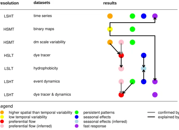
were used to investigate soil moisture response patterns and thus flow in the unsaturated zone. This included the analy-sis of yearly soil moisture dynamics as well as of event re-sponse patterns resulting in the deduction of flow processes, the use of rainfall simulation experiments with dye tracers to corroborate these deductions, but also the analysis of re-sponse times at the event scale. The episodic measurements along the hillslope transects allow for the analysis of spatial patterns and their long-term dynamics for 14 locations and 6 depths and for the investigation of small scale soil moisture variability at the decimeter scale. Figure 2 gives an overview of the data sets used in this study. The synergies arising from their combination are described in Sects. 4 and 5.
3.2 Streamflow, groundwater levels and rainfall
LSHT
HSMT
HSMT
HSLT
LSLT
LSHT
LSHT
time series
binary maps
dm scale variability
dye tracer
hydrophobicity
event dynamics
dye tracer & dynamics
resolution datasets results
Legend
higher spatial than temporal variability low temporal variability
preferential flow
preferential flow (inferred)
persistent patterns seasonal effects
seasonal effects (inferred) fast response
confirmed by explained by
Fig. 2.Overview of data sets used in this study, along with their temporal and spatial resolution, main results and synergetic effects. (L-low,
M-medium, H-high, S-spatial, T-temporal)
3.3 Soil moisture profiles
To investigate the dynamics as well as the trends in soil mois-ture profiles along the hillslope, measurements were carried out at two transects with FDR (frequency domain reflectome-try) profile probes (Delta-T) in 10, 20, 30, 40, 60 and 100 cm depth. Both transects are located on the eastern slope close to the main stream gauging station S1 (Fig. 1). This hills-lope was selected for being quite typical for the catchment in slope and vegetation as well as for its accessibility. At each depth soil moisture is measured in a soil volume of about 2500 ccm, a cylinder with a radius of 10 cm. The absolute measurement error of about 3% (as given by the manufac-turer) is for the measurement of the dynamics of soil mois-ture of less importance. The error of the measured dynamics, i.e. the error of the values relative to each other is likely to be smaller than the absolute error. As a result of the special characteristics of the volcanic ash soil, such as the extremely high porosities and the fact that volcanic glass is a primary constituent, the built-in standard calibrations were not appli-cable. It was thus necessary to calibrate the probe specifically for this type of soil with gravimetrically determined water contents of 19 soil samples of the upper horizons (horizons 1 and 2 in Table 1), which generally cover depths from 5 to 130 cm. Water contents for the calibration curve ranged from 16 to 51 Vol%. The calibration resulted in a correction of the supplied generalised soil calibration given by the
man-ufacturer: θcorr=0.8126×θ+0.1145. With this calibration curve it was possible to reproduce the gravimetrically deter-mined values with anR2of 0.94 and a median absolute error of only 1 Vol%. These profile probes do not measure within a purely circular field as the sensor only extends about two thirds around the probe. For manual measurements it is pos-sible to cover the full circle by taking three measurements, turning the probe by 120◦
carried out at 41 occasions at irregular time intervals dur-ing field campaigns (December 2003–February 2004, Octo-ber 2004–DecemOcto-ber 2004, NovemOcto-ber 2005–DecemOcto-ber 2005 and April–May 2006).
3.4 Rainfall simulation experiments
To investigate subsurface flow patterns 10 dye tracer exper-iments with brilliant blue were carried out in the Malalc-ahuello catchment in 2004 and 2005 (for details see Blume et al. (2008b)).
Furthermore, similar rainfall simulation experiments were conducted in May 2006 at the locations of the continuously measuring soil moisture probes. It was thus possible to test our perception of flow in the unsaturated zone at these pro-files. The plot size was 1.2 m×1.2 m with the probe situated in the center. For all experiments the dye tracer Brilliant Blue with a concentration of 4 g/l was used. The dye was applied with a hand pressurized pesticide sprayer in order to simu-late rainfall. 30 l of the dye were sprayed over a period of 3 h. This corresponds to a total of 25 mm at application rates of 8.3 mm/h on average. Profiles of the plots were excavated the following day and photos of the dye patterns were taken with a digital camera.
3.5 Response times
Response times were calculated for both, dry and wet season from the time series of rainfall, soil moisture, groundwater levels at well W1 (Fig. 1) and streamflow (all with 10 min resolution). Response time in this case was defined as the time period between begin of precipitation and first response of soil, ground- and stream water. The following threshold values were chosen to identify the point of first response in the time series: an increase of 0.2 Vol% in soil moisture, an increase of 0.005 m in groundwater level and an increase of 0.01 m3/s in stream flow. As the main interest are the rel-ative changes in response times from winter to summer, the absolute values of these thresholds are of less importance as long as consistent thresholds (>noise of the time series) are used for the entire analysis.
3.6 Data analysis
Data was analyzed at different space-time scales using vari-ous graphical methods. The space-time scales analyzed in-cluded event and longterm scale, point and hillslope scale.
Simple line plots were used to analyze annual dynamics as well as small scale variability of soil moisture.
Soil moisture patterns at the hillslope scale are investigated with the help of binary indicator maps for each depth. These maps show locations where soil moisture is above/below a certain threshold. Here we selected the median value to in-dicate wetter/drier than average locations as well as the 75% quantile to indicat wet spots. These thresholds are calculated
for each depth and sampling occasion at all sampling loca-tions on both transects and depend thus on time and depth. The temporal aspect of these binary patterns is included in the indicator map by plotting location on the slope on the y-axis and time on the x-y-axis, thus giving an idea of pattern persistency.
Event scale datasets with 10 min temporal resolution were analyzed with the help of colour maps which included tem-poral dynamics similar to those used by Weiler and Naef (2003). Here, time is plotted on the x-axis while depth is plotted on the y-axis. Soil water content at each depth and point in time is visualized by color, changing from blue to red with increasing wetness. For additional information the response of streamflow and groundwater, as well as the rain-fall intensity at each point in time were also included. Color scales were adapted from one event to the next in order to get the best “color resolution” possible, producing clearer pat-terns of response. It thus becomes possible to explore and identify patterns in moisture response, patterns in spaceand time that are much more difficult to identify in the classical line plots of soil moisture dynamics. In a next step flow pro-cesses were deduced from these patterns.
3.7 Estimation of potential for self-reinforcing flow paths
interface (Eq. 1), these flow paths are likely to persist over time.
Kθ(flow path) [m/s]
Kθ(interface) [m/s]
≫1ψ(interface) [cm H2O/cm]
1 [cm H2O/cm] (1) 3.8 Hydrophobicity
Potential hydrophobicity was measured with the Water Drop Penetration Time (WDPT) test as described in Dekker and Ritsema (1994) for 12 air dried soil samples from 4 different locations and depths from 5 to 80 cm. The WDPT test is a simple test for the persistency of water repellency where a water drop is applied to a soil sample and the time between application of the water drop and its penetration into the soil is measured. Water drop penetration times for air dried soil have been classified by Dekker and Ritsema (1994) into 5 classes: wettable (<5 s), slightly water repellent (5–60 s), strongly water repellent (60–600 s), severely water repellent (600–3600 s) and extremely water repellent (>3600 s). Af-ter testing if a soil sample was wettable soil samples show-ing water repellency were submitted to 12 repetitions of the WDPT, each test carried out with a different subsample.
4 Results and discussion
4.1 Annual dynamics of soil moisture
The annual dynamics of soil moisture, shown for the period from October 2004–May 2006 in Fig. 3, are little pronounced in comparison to the event dynamics. Only during the sum-mer months (February 2005 and February 2006) a short dry-ing period can be observed (Fig. 3). However, as soon as the first rainfall starts in autumn, soil moisture values rebound to their previous level. Overall, the temporal variability of soil moisture at each of the sensors is much lower than the spatial variability along the depth profile (see also Blume et al. (2008a), for more detailed statistics on this topic). The profile at probe 1 (lowest on the slope) had generally higher moisture contents, but otherwise no trends along the transect could be established. Interestingly, events that lead to strong responses in discharge and groundwater level (e.g. in May and June 2005), do not show a comparably strong response in soil moisture (Fig. 3). As even the slope groundwater (well 5 – for location see Fig. 1) responds strongly, this difference in response can not be attributed to snow melt events in the upper part of the catchment. A more likely explanation is that the unsaturated subsurface in this catchment is close to equilibrium or steady state (see also the explanations to event 3, in Sect. 4.4). This means that soil moisture change is close to zero, but waterflow itself is non-zero. Perturbations of rainfall and drought only lead to small and short responses in soil moisture as water is efficiently being transported to greater depths. While this efficient transport of water in the
unsaturated zone only results in small changes in soil mois-ture in the upper meter, it also leads to a fast and pronounced response in ground and surface water.
Subsurface flow for the three events indicated with arrows in Fig. 3 is analyzed in more detail in Sect. 4.4.
4.2 Soil moisture spatial patterns at the hillslope scale
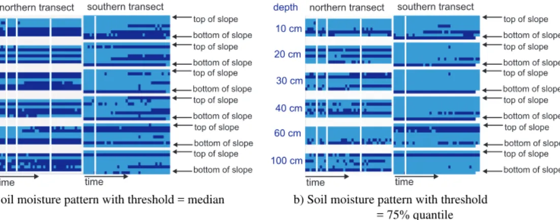
Using the manually measured soil moisture profiles as well as the corresponding logged data sets it was possible to estab-lish a picture of spatial as well as coarse resolution temporal soil moisture characteristics. Soil moisture patterns at the two transects are depicted in Fig. 4 using the binary indicator maps.
Surprisingly, no general trends along the transects could be identified, apart from for the 10 cm sensors: There seems to be a correlation with position on the slope for the 10 cm depth, but not for the deeper sensors. At 10 cm depth the lower half of the slope is generally wetter than the upper part of the slope. This is probably due to shading effects: the deeper in the steep valley the fewer hours of direct sunshine. Another possible explanation is downslope flow accumula-tion in the o-horizon. The northern transect is wetter than the southern transect, which is probably due to denser vege-tation. It was found that spatial patterns are generally persis-tent over time.
4.3 Variability of soil moisture at the decimeter scale and preferential flow patterns
time time
northern transect southern transect
10 cm 20 cm 30 cm 40 cm 60 cm 100 cm depth
top of slope
bottom of slope top of slope
bottom of slope
top of slope
bottom of slope top of slope
bottom of slope top of slope
bottom of slope top of slope
bottom of slope
time time
northern transect southern transect
10 cm 20 cm 30 cm 40 cm 60 cm 100 cm depth
top of slope
bottom of slope top of slope
bottom of slope
top of slope
bottom of slope top of slope
bottom of slope top of slope
bottom of slope top of slope
bottom of slope
a) Soil moisture pattern with threshold = median b) Soil moisture pattern with threshold
= 75% quantile
Fig. 4. Manual soil moisture measurements at irregular intervals at 41 occasions during the field campaigns (December 2003–February
2004, October 2004–December 2004, November 2005–December 2005 and April–May 2006). The northern transect is shown on the left, the southern transect is shown on the right. Each block corresponds to one depth on that particular slope. Sensors are ordered as follows: lowest sensor on the slope is plotted on the lowest line of a single block. On the left transect there are 6 sensors, on the right transect there are 8 sensors. y axis is position on the slope (within bars) and depth (from one bar to the next), x axis is time (i.e. the 41 temporally irregularly spaced data points). Dark blue indicates measurements of soil moisture above the median(a)or the 75% quantile(b)of that depth, light blue are values below these thresholds. Missing data is indicated with white fields.
0.10 0.20 0.30 0.40 0.50 0.60
1 2 3 1 2 3 1 2 3 1 2 3 1 2 3 1 2 3 1 2 3 1 2 3 1 2 3 1 2 3 1 2 3
22.10.04 08.12.04 13.11.05 18.11.05 25.11.05 30.11.05 05.12.05 13.12.05 30.04.06 05.05.06 06.05.06
so
il
m
o
ist
u
re
[
m
³/
m
³]
H4_10
H4_20
H4_30
H4_40
H4_60
H4_100
a) H4
0.10 0.20 0.30 0.40 0.50 0.60
1 2 3 1 2 3 1 2 3 1 2 3 1 2 3 1 2 3 1 2 3 1 2 3 1 2 3 1 2 3 1 2 3
22.10.04 08.12.04 13.11.05 18.11.05 25.11.05 30.11.05 05.12.05 13.12.05 30.04.06 05.05.06 06.05.06
so
il
m
o
ist
u
re
[
m
³/
m
³]
H5_10
H5_20
H5_30
H5_40
H5_60
H5_100
b) H5
Fig. 5. Directional or small scale variability at manual measurement points H4 and H5. Measurements 1, 2, 3 at each date are repetitions
Table 2. Results of the Water Drop Penetration Time (WDPT) test. If a sample showed water repellency the WDPT test was carried out with 12 repetitions, i.e. with 12 sub-samples. Shown are the number of tests per sample falling in the different classes of water repellency. Samples “forest 1-3” were taken at the slope of the soil moisture transect, while samples named “pine” were taken in a pine plantation downstream of the catchment outlet. The sampling sites of “forest 1–3” do not correspond to the locations of the soil moisture probes 1–3.
location depth wettable slightly strongly severely extremely (cm) water repellent water repellent water repellent water repellent
forest 1 5–10 no – – 5 7
forest 1 10–15 no – 2 3 7
forest 2 10–20 no – 12 – –
forest 2 20–60 yes – – – –
forest 2 60–80 yes – – – –
forest 3 10–20 no 3 9 – –
forest 3 20–60 yes – – – –
forest 3 60–80 yes – – – –
pine 0–5 no – – – 12
pine 5–20 no 12 – – –
pine 20–60 yes – – – –
pine 60–80 yes – – – –
WET SEASON
DRY SEASON
Fig. 6. Preferential flow paths marked during dye tracer experiments. Flow patterns differ from wet to dry season, especially in the top
20 cm. For details see Blume et al. (2008b).
study in this catchment (Blume et al., 2008b), where pref-erential flow proved to be the rule for all forested sites (9 experiments), with slightly varying flow patterns during dry and wet season (Fig. 6). If a soil moisture sensor was located near the interface of such a preferential flow path, soil mois-ture would differ considerably depending on the direction of the measurement. The scale or width of the flow paths iden-tified with the dye tracer is in the order of<3 decimeters, thus matching the scale of the measurement. A sensor show-ing no directional variation must therefore be located either in the center of a flow path or in the center of the matrix with no flow path within reach of the measurement. Ritsema and Dekker (1996) also used small scale (5–10 cm) variabil-ity of soil moisture as a measure for preferential or finger flow. In their study moisture gradients between flow paths and non-flow areas ranged between 3 and 6 Vol%. Assuming small scale soil moisture variability does indeed indicate the presence of a preferential flow path, the fact that in
Malalc-ahuello 68% of all sensors show this type of variability also gives us a measure of the importance of preferential flow in this catchment.
There are five possible explanations for the surprising per-sistency of the small scale soil moisture patterns (or prefer-ential flow patterns) over the course of more than one and a half years (Fig. 5):
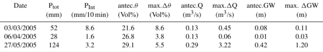
Table 3. Response characteristics and antecedent conditions for the three events shown in Fig. 7 (Ptot= rainfall amount, PInt= maximum
rainfall intensity, antec.θ= antecedent mean soil moisture content for the top 30 cm, max.1θ= max. increase in soil moisture of all sensors, antec.Q = antecedent streamflow, max.1Q = max. increase in streamflow, antec.GW = antecedent groundwater level at well W1 relative to the well datum at 2.55 m below the soil surface, max.1GW = max. rise in groundwater levels).
Date Ptot PInt antec.θ max.1θ antec.Q max.1Q antec.GW max.1GW
(mm) (mm/10 min) (Vol%) (Vol%) (m3/s) (m3/s) (m) (m)
03/03/2005 52 8.6 21.6 8.6 0.13 0.45 0.08 0.11 06/04/2005 28 1.6 26.8 3.8 0.13 0.06 0.01 0.03 27/05/2005 124 3.2 29.1 5.5 0.29 3.22 0.42 1.20
2. They might also be due to textural differences. How-ever, as the sensors have only a range of 10 cm the mea-sured volume is likely to be located within a single layer. 3. These patterns might also be induced by roots, which are not likely to change position on this time scale. However, roots were only found in some of the in-stances where these preferential flow patterns were ob-served during dye tracer experiments.
4. They might be due to hydrophobicity in some parts of the soil, which would produce self reinforcing patterns likely to persist if not subjected to long periods of sat-uration. The change in flow patterns from dry to wet season, which was found in the dye tracer experiments (Fig. 6, for details see Blume et al., 2008b), supports this theory (Fig. 2). Potential water repellency of soil samples from 5 to 80 cm depth was tested with the Wa-ter Drop Penetration Time test. It was found that while the top horizons show strong to extreme potential wa-ter repellency, samples from greawa-ter depths are wettable (Table 2). However, this test determines only poten-tial water repellency, measured in air dried soil. Hy-drophobicity under field conditions is likely to be less pronounced and spatially heterogeneous as a result of water redistribution by canopy, litter, microtopography or by variability in soil organic matter (Dekker and Rit-sema, 1994; Ritsema and Dekker, 1995). The O-horizon in this catchment only has a thickness of about 5 cm, but due to its higher organic matter content, it is likely to enforce redistribution processes due to spatially hetero-geneous water repellency.
5. These patterns could also be self reinforcing due to the strong gradient in soil moisture itself, leading to faster vertical transport within the wetter area (the flow path) than lateral flow into the drier area as a result of the gradient in matric potential.
Possibility no.5 was investigated with a simple estimation: If the ratio of the of the unsaturated hydraulic conductivities is much larger than the gradient in matric potential across the interface (Eq. 1), flow paths are likely to be self-reinforcing
and persistent over time. This estimation was carried out by calculating the unsaturated conductivities for a number of gradients in soil moisture and thus matric potential: from 20 to 25 Vol%, from 25 to 30 Vol% and from 30 to 35 Vol%, thus covering the range from 20 to 35 Vol% of soil moisture, where most of the variability was observed. The gradient of 5 Vol% chosen to investigate this phenomenon was in the upper range of gradients observed in the field.The gradient in potential within the flow path is assumed to be equal to 1 [cm H2O/cm]. It was found that flow paths would indeed be self-reinforcing for a pure sand (with a ratio ofKθ up to 11 times larger than the ratio of1ψ), however, in these ash soils, which have a fraction of at least 20% silt, it is very dif-ficult to achieve these conditions (the ratio ofKθ is less than half that of the ratio of1ψ). It is thus unlikely that solely the gradient in soil moisture causes the flow paths to persist in time. Nevertheless, if the unsaturated conductivity across the interface is further diminished by the effects of hydropho-bicity a persistant pattern becomes more probable. Further-more this type of soil is known to be hysteretic (Shoji et al., 1993; Musiake et al., 1988) thus causing a shift in the wet-ting curve compared to the here used draining curve, which could also change the outcome of this rough estimation. Per-sistent fingers as a result of hysteresis of the soil moisture characteristic curves were described by Selker et al. (1996) and Nieber (1996). Nieber (1996) explains that fingers will persist if the water entry pressure on the main wetting curve is smaller then the air entry pressure on the main drainage curve. However, due to lack of information on the main wet-ting curve, this effect cannot be assessed for the soils in the Malalcahuello Catchment.
4.4 Soil moisture dynamics on event basis
Rainfall Discharge Groundwater level Probe 3 Probe 2 Probe 1 10 20 30 40 60 100 cm depth
Rainfall
[mm/10min]
GW level
[cm]
Discharge
[m /s]3
Soil water [Vol%] 0 >4 6 17 0.1 0.6 0 9 10 20 30 40 60 100 cm depth 10 20 30 40 60 100 cm depth
time 1
2 2
0 20 40 1 0.6 0.4 0.3 0.2 0.1
0 20 40
depth [m] 1 0.6 0.4 0.3 0.2 0.1
0 20 40
antec. soil moisture [%]
1 0.6 0.4 0.3 0.2 0.1 March median
a) Rainfall event 3 March 2005.
Rainfall Discharge Groundwater level Probe 3 Probe 2 Probe 1 10 20 30 40 60 100 cm depth
Rainfall
[mm/10min]
GW level
[cm]
Discharge
[m /s]3
Soil water [Vol%] 0 >4 1 4 0.1 0.2 0 4 10 20 30 40 60 100 cm depth 10 20 30 40 60 100 cm depth
time
3
4
4 0 20 40
1 0.6 0.4 0.3 0.2 0.1
0 20 40
depth [m] 1 0.6 0.4 0.3 0.2 0.1
0 20 40
antec. soil moisture [%]
1 0.6 0.4 0.3 0.2 0.1 April median
b) Rainfall event 6 April 2005.
time Rainfall Discharge Groundwater level Probe 3 Probe 2 Probe 1 10 20 30 40 60 100 cm depth
Rainfall
[mm/10min]
GW level
[cm]
Discharge
[m /s]3
Soil water [Vol%] 0 >4 42 162 0.3 3.5 0 5 10 20 30 40 60 100 cm depth 10 20 30 40 60 100 cm depth
5
6 0 20 40
1 0.6 0.4 0.3 0.2 0.1
0 20 40
depth [m] 1 0.6 0.4 0.3 0.2 0.1
0 20 40
antec. soil moisture [%]
1 0.6 0.4 0.3 0.2 0.1 May median
c) Rainfall event 27May 2005.
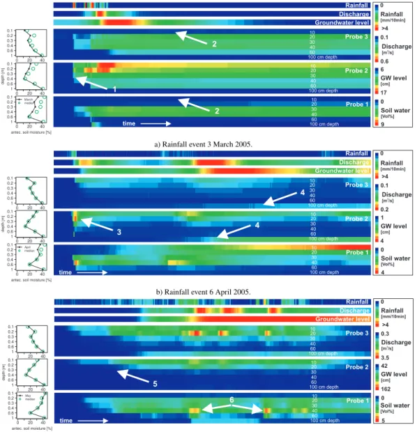
Fig. 7. Event response patterns of soil moisture for three rainfall events. Time is plotted on the x-axis. All plots show a two day period.
Explanation of color bars from top to bottom: The uppermost bar shows 10-min rainfall intensity: dark blue is equivalent to 0 mm/10 min, dark red is equivalent to≥4 mm/10 min. The two following bars show the increase of discharge and rise of groundwater level (at well W1), respectively. The color scale is stretched from minimum to maximum values. Down below follow the three wide bars representing the soil moisture response at the hillslope transect. The upper bar corresponds to the profile probe at the upper end of the slope (P3), the middle bar to the mid-slope probe (P2) and the lowest bar to the profile probe at the lower end of the slope (P1). Within these three wide colour bars, each stripe corresponds to a certain depth: 10, 20, 30, 40, 60 and 100 cm. 0 on the soil water color scale corresponds to antecedent moisture content. The arrows indicate the most prominent features and are numbered for easier reference. The small plots to the left of each soil moisture bar show antecedent moisture conditions for each depth as well as the median values of soil moisture content as reference.
Three typical events are shown in Fig. 7. The timing of the events is indicated by arrows in Fig. 3. Probe 1 is located at the lower end and probe 3 at the upper end of the hillslope transect. Details of event response and antecedent conditions are listed in Table 3.
For the first event, the event on 3 March 2005 (Fig. 7a), total precipitation amounted to 52 mm with a highest
Rainfall
Probe 3
Probe 2
Probe 1
10 20 30 40 60 100 cm depth
Rainfall
[mm/10min]
Soil water
[Vol%]
0
>4
0
6
10 20 30 40 60 100 cm depth 10 20 30 40 60 100 cm depth
A)
B)
C)
time
0 20 40
1 0.6 0.4 0.3 0.2 0.1
0 20 40
depth [m]
1 0.6 0.4 0.3 0.2 0.1
0 20 40
antec. soil moisture [%] 1
0.6 0.4 0.3 0.2 0.1
May06 median
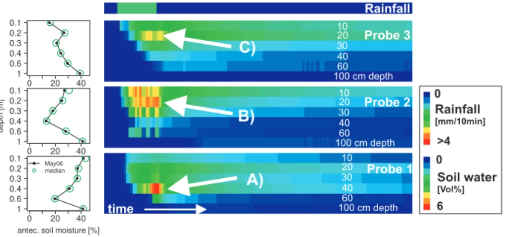
Fig. 8.Rainfall simulation with dye tracer at the locations of the soil moisture probes: amount of dye applied: 25 mm, intensity of application:
8.3 mm/h. The arrows A, B and C mark the most prominent patterns observed during this simulated rainfall event. The time scale of this plot has a length of one day.
1 in Fig. 7a), due to high rainfall intensities and high hy-draulic conductivities, and b) very little reaction at the 10 cm depth for probes 1 and 3 (arrow 2 in Fig. 7a). This is proba-bly due to hydrophobicity resulting from the dry antecedent moisture conditions. This pattern was observed only for the 3 driest occasions. The dry antecedent conditions also make steady state conditions unlikely, where flow without change in moisture content is possible. Soil moisture increase be-low the hydrophobic layer thus must be due to lateral inputs, either at the the decimeter scale or at the hillslope scale.
The rainfall event on April 6th 2005 (Fig. 7b) has a total precipitation of 28 mm and only low rainfall intensities. The maximum increase in soil moisture, as well as streamflow and groundwater levels are low with 3.8 Vol%, 0.06 m3/s and 3 cm, respectively (Table 3). Antecedent moisture contents correspond to the median values for most depths, apart from the 10 and 20 cm depths at probe 1. The major patterns iden-tified for this event are: a) fast vertical water transport, due to high hydraulic conductivities (arrow 3 in Fig. 7b), and b) late but persistent response at 100 cm depth for probes 2 and 3, while no such reaction can be seen at the 60 cm sensor (arrow 4 in Fig. 7b). As water is apparently not transported to this point vertically, this seems to be the result of lateral water input, causing a slow trailing “wave” at this depth.
The event on 27 May 2005 (Fig. 7c) has a very high total precipitation of 124 mm with a highest intensity of 3.2 mm/10 min. However, as this event is probably a rain on snow event, it is difficult to estimate the actual amount of water entering the soil. Antecedent moisture contents are high (at or above median values). While the response of dis-charge (3.22 m3/s increase), and ground water levels (120 cm increase) is extremely strong, soil moisture shows a much less pronounced reaction. One possible explanation is that this is not only an event with high rainfall amounts, but that snow was also present in the catchment at this time (30 cm of
snow were measured at the climate station just outside of the research catchment at 1270 m elevation, while the soil mois-ture transect is located at about 1140 m elevation.). Therefore some of the runoff might be generated at the snow surface or within the snow layer. However, the extreme response at well W5 (see also Fig. 3) proves that large amounts of water did indeed enter the subsurface. A more likely explanation is therefore that as all water in excess of field capacity is being transported quickly to greater depths, soil moisture increases most for dry antecedent conditions and less in conditions of high antecedent wetness despite the fact that large amounts of water are being transported during nearly steady state flow conditions. This efficient vertical water transport will result in a pronounced response in the saturated zone without caus-ing similarly pronounced peaks in moisture content. The most prominent patterns for this event are: a) slow verti-cal water transport, probably due to lower rainfall intensities (arrow 5 in Fig. 7c and b) strong response at 40 cm depth for probe 1, very local and short-term (arrow 6 in Fig. 7c). This reaction might be due to an underlying capillary barrier, causing the water to pond above it until breakthrough. This pattern was observed at this location quite frequently (for 15 events out of 34).
4.5 Dye tracer rainfall simulation
1 m
1
2
3
1 m
1
2 3
(a) Flow paths at profile probe 1 (b) Flow paths at profile probe 2
1 m
1
2
(c) Flow paths at profile probe 3
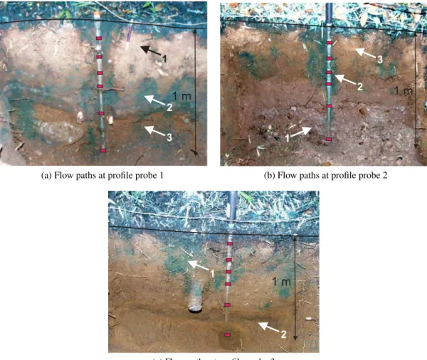
Fig. 9. Flow path visualization at the locations of the three continuously logging profile probes. The black line indicates the soil surface
and the arrows the most important features in each photo. They are numbered for easier reference. The red lines indicate the approximate location of the soil moisture sensors.
of application as for the rainfall intensities in Fig. 7. Nei-ther streamflow nor groundwater level dynamics are plotted as there was no reaction to these small scale experiments (small in comparison to the size of the hillslope). Antecedent moisture contents are quite high (at median values for all but the 10 cm sensors at probes 1 and 2). The dynamic mois-ture response patterns show fast/preferential vertical flow for probes 1 and 2 and slow vertical water transfer for probe 3 (Fig. 8). One day after the sprinkling experiment, cross sec-tions of the infiltration plots were excavated and the dye stain patterns marking the flow paths of the dye in the unsaturated zone were photographed. The three photos of the cross sec-tions at the locasec-tions of the soil moisture probes are shown in Fig. 9. Preferential flow is found at all three plots (com-pare Fig. 2). Flow occurred in plumes, which are separated by distinct areas of little or no flow unmarked by blue dye.
Figure 9a shows the flow paths of probe 1 (located at the bottom of the slope). While blue dye can be seen in the top 5 cm, hardly any dye stains could be found in depths of 5–
1 0.6 0.4 0.3 0.2 0.1
0.0 0.2 0.4
Probe 3
soil moisture [m³/m³]
depth [m]
Q GW S40 S30 S20
0 5 15
Winter: P3 (n=19)
response lag [h]
Q GW S40 S30 S20
0 5 15
Summer: P3 (n=8)
response lag [h]
1 0.6 0.4 0.3 0.2 0.1
0.0 0.2 0.4
Probe 2
soil moisture [m³/m³]
depth [m]
Q GW S40 S30 S20
0 5 15
Winter: P2 (n=19)
response lag [h]
Q GW S40 S30 S20
0 5 15
Summer: P2 (n=8)
response lag [h]
1 0.6 0.4 0.3 0.2 0.1
0.0 0.2 0.4
Probe 1
soil moisture [m³/m³]
depth [m]
Q GW S40 S30 S20
0 5 15
Winter: P1 (n=19)
response lag [h]
Q GW S40 S30 S20
0 5 15
Summer: P1 (n=8)
response lag [h]
Fig. 10.Soil moisture variability along each profile as well as lag times of response in soil moisture, discharge (Q) and groundwater levels
(GW) for 19 events in winter and 8 events in summer. Soil moisture response times are shown for 20, 30 and 40 cm depth (S20, S30, S40).
flow patterns caused by water repellency of the soil. In late summer the 10 cm and sometimes also the 20 cm sensor are surrounded by hydrophobic soil (Fig. 7a and b).
The cross section at probe 2 (Fig. 9b) shows as most dis-tinct feature the saprolite layer (weathered bedrock) starting at the location of the 60 cm sensor (arrow 1 in Fig. 9b). The 100 cm sensor is thus located within the saprolite. It was also found that the probe is located within a preferential flow path coinciding with a concentration of fine roots (arrow 2 in Fig. 9b). Maximum infiltration depth is about 80 cm in the three major plumes. A hydrophobic layer with very little staining can be seen in the cross section (arrow 3 in Fig. 9b). However, this layer was not identified in the soil moisture
data, as the probe is located within the preferential flow path and not in a hydrophobic patch. The high velocity of flow and the strong response in this preferential flow path is also visible in Fig. 8 (arrow B) and was also a feature of the soil moisture response space-time maps at this location.
and a layer of fine gravel (arrow 2 in Fig. 9c), thus prob-ably measuring in both layers, while the 100 cm sensor is situated in a layer of more compacted silty sand starting at a depth of approx. 75 cm. Maximum depth of infiltration is 80 cm. The fact that the layer at the 100 cm sensor is more compacted might explain why reaction at this sensor occurs delayed and prolonged. This would correspond to lower hy-draulic conductivities in the compacted layer causing a delay in response and a prolonged peak. However, as the response at the 60 cm sensor is often very weak, the water causing the peak at 100 cm depths is most likely transported to this point not vertically but laterally. The dense root zone in the top 20 cm explains the strong reaction at the 20 cm sensor (Fig. 8, arrow C). Probe 3 shows a slower reaction to rainfall compared to the other two probes (Fig. 8 and also Fig. 7), which is explained by the fact that this probe is not situated within a preferential flow path.
4.6 Response times
To test if the seasonal change in subsurface flow has an ef-fect on overall catchment response, response times for soil moisture, groundwater and stream flow were calculated for the wet and dry season separately (Fig. 10). This analysis is based on 27 rainfall events between December 2004 and April 2006. S20, S30, S40 are the response lags of the soil moisture sensors at 20, 30 and 40 cm depth, GW is the re-sponse lag of ground water level at well W1 (Fig. 1) and Q is the response lag of stream flow. Groundwater response is generally slower than stream flow response. (At this hills-lope the groundwater surface at well W1 in the vicinity of the stream is generally about 60 cm below the level of the stream bed.) Surprisingly, the soil moisture sensors often react slower than stream flow. This could either mean that rainfall is not uniformly distributed over the catchment or that these sensors are bypassed by preferential flow paths. Surface runoff is unlikely, due to high infiltration rates and porosities and has not been observed during field campaigns. Another possible explanation would be lateral flow in the duff layer/organic horizon. Response lags of all parameters show similar behavior over time: response times are short from January to April (summer and early fall) when com-pared to the winter months. This is probably the result of higher rainfall intensities on the one hand (median maximum intensities are 2.1 mm/10 min in winter and 3.0 mm/10 min in summer) and enhanced preferential flow due to hydrophobic-ity on the other hand. Snow was present/melting during 4 of the winter events, however, this does not lead to a consistent change in response time: both, faster and slower than median responses have been observed for these events. Streamflow response times for the events shown in the space-time colour maps (Fig. 7) range from 30 minutes for the first event (driest antecedent moisture conditions), 1:50 h for the second event up to 6:40 h for the event in May (wettest antecedent condi-tions).
5 Summary and conclusions
The soil moisture data obtained in this study provided diverse insights in subsurface flow and runoff generation processes in this catchment. It was shown that high resolution time series of soil moisture in combination with manual measure-ments at irregular time intervals can be a valuable addition to time series of precipitation and discharge when investigating runoff generation processes. This is especially true for catch-ments where only short time series of data are available, as in the Malalcahuello Catchment. The approach of combining datasets with different spatio-temporal resolution allowed for the investigation of soil moisture dynamics as well as pat-terns and proved to be less expensive than high density in-stallation of continuously logging sensors while also being applicable to difficult terrain, i.e. densely forested and steep hillslopes. The synergetic effects achieved with this combi-nation of datasets is visualized in Fig. 2.
The time series of soil moisture for the 19 month period in Fig. 3 show that spatial variability of soil moisture is much higher than its temporal variability. Both, rainfall events and droughts only cause small, fast and short perturbations and the moisture content quickly rebounds to previous lev-els. This behaviour corresponds to a system at or close to a dynamic equilibrium, i.e. close to steady state flow condi-tions in the subsurface. This seems to prevail most time of the year. This is corroborated by the high annual precipita-tion, high baseflow index and annual runoff and the very low event runoff coefficients.
The use of space-time colour maps facilitated the analysis of soil moisture response dynamics, especially concerning the timing and extent of response along the vertical profile. It was thus possible to identify a number of patterns which can be attributed to different phenomena of flow in the un-saturated zone. The very subdued response of soil moisture in the upper soil horizon at two locations during the driest period (late summer) was attributed to the formation or re-inforcement of hydrophobicity in this layer. The accumula-tion/ponding of water at certain depths was assumed to be due to the effect of capillary barriers. This was confirmed by the dye tracer experiment carried out at this location.
Strong response at certain depths while the layers just above show little reaction indicate the importance of lat-eral flow processes. However, we do not know on what scale these thus “observed” lateral flow paths are active (sev-eral decimeters, meters or hillslope scale). Lat(sev-eral flow has also been directly observed in a dye tracer experimenet with an application intensity of 20 mm/h. Here lateral flow oc-curred in the duff layer (Blume et al., 2008b). The short response times of streamflow also indicate that lateral sub-surface storm flow is likely to be important.
Persistency of potential water repellency was found to be strong to extreme for the upper horizon. Hydrophobicity has also been observed in Chilean young volcanic ash soils by other researchers (Bachmann et al., 2000; Ellies, 1975) and is also of importance in volcanic ash soils of Ecuador (Poulenard et al., 2004). In addition, differences in flow pat-terns from dry to wet period were found in the Malalcahuello Catchment during a more extensive study involving a total of 10 dye tracer experiments (Blume et al., 2008b). The change in flow pattern observed in this study further supports the theory that preferential flow in this catchment is reinforced by hydrophobicity (application intensities were the same for dry and wet season experiments). Similar flow patterns also attributed to hydrophobicity were observed in other studies (Ritsema and Dekker, 2000; Ritsema et al., 1998; Ritsema and Dekker, 1994; Dekker and Ritsema, 2000; de Rooij, 2000). The fact that throughfall amounts are highly heteroge-nous in this catchment (Blume et al., 2008a) is likely to be the reason why some locations (probably on the decimeter scale) are drier than others and thus more likely to develop water repellency. Spots of high water input are therefore likely to become preferential flow paths. These observed patterns in dynamics were found to be spatially and temporally persis-tent insofar as the event pattern dynamics of soil moisture observed in Fall 2005 (Fig. 7) matched well with the flow pat-terns found during the dye tracer experiments one year later. The persistency of the spatial patterns of soil moisture for 14 locations and 6 depths (Fig. 4) shows that spatial variability is much higher than temporal variability and that wetter lo-cations are likely to remain wet. Furthermore the patterns of soil moisture variability at the decimeter scale, which were attributed to the presence/absence of preferential flow paths, were also found to be persistent over a period of more than one and a half years. The stationarity of these flow patterns is another indicator that steady state conditions prevail in this catchment.
Hydrophobicity is the most likely explanation for the flow patterns found here. However, the effects of hydrophobicity are probably aggravated by root channels, strong gradients in matric potential and the hysteresis of the soil moisture char-acteristic curves of volcanic ash soils as described by Shoji et al. (1993).
The last and maybe most important question is the ques-tion of how important this locally observed preferential flow is for the system as a whole, i.e. runoff response/runoff gen-eration at the catchment scale.
The small response of soil moisture dynamics to pertur-bations as well as persistency/stationarity of flow paths cor-roborate our perception that this undisturbed, forested catch-ment is at or close to steady state, i.e. a dynamic equilibrium. This perception was originally based on integral observations such as the fact that we observe high annual runoff and a high baseflow index, while event runoff coefficients are low, and has now been corroborated by internal observations, e.g. soil moisture response and flow patterns. Efficient water
trans-port, as observed locally, therefore would indeed have an ef-fect at the catchment scale.
Several additional findings indicate that while preferential flow was only observed at the plot scale it might indeed be an important factor of runoff generation at the catchment scale. That preferential flow occurs throughout the catchment is in-dicated by the fact that additionally to the three tracer experi-ments shown in this study all 9 dye tracer experiexperi-ments carried out under forest at various locations in the catchment showed preferential flow patterns (Blume et al., 2008b). The fact that 68% of the sensors at the 11 manual measurement points showed small scale soil moisture variability is another indi-cator for the importance of these preferential flow paths. Last but not least the analysis of response times for soil moisture, groundwater and streamflow reveiled that response lags are generally much shorter during the summer months were pref-erential flow is also likely to be further enforced by stronger hydrophobicity. Interestingly streamflow often shows faster response than both groundwater and soil water. This might be due to non-uniform rainfall distribution (i.e. earlier onset of rainfall further up in the catchment causing stream levels to respond while soil moisture at the slope close to the catch-ment outlet remained unchanged). However, as soil mois-ture response measurements are restricted to only three lo-cations it is also likely that there are other preferential flow paths with even faster response than the ones measured by our instruments. In this case preferential flow in the verti-cal and then a fast reaction along a horizontal layer interface might be the reason for the short response lags of stream-flow found in this catchment. (Finger stream-flow is known to cause faster breakthrough as investigated by de Rooij and deVries (1996) in a modelling study.) The question whether or not these preferential flow processes are important for catchment response could be investigated further by application of a physically based hydrological model either on the hillslope or on the catchment scale.
To summarize the main conclusions in short:
1. the synergy of soil moisture datasets with different spatio-temporal resolution proved to be useful for the investigation of subsurface flow processes. Continu-ously monitored rainfall experiments at the location of the moisture probes with subsequent excavation of dye stained soil profiles facilitated testing/corroboration of the perception of subsurface flow gained from the mois-ture patterns.
2. data-visualization with space-time colour maps permits a much more detailed analysis of soil moisture response than simple line plots alone
3. soil moisture/flow patterns in the here investigated young volcanic ash soils were shown to be persistent in time and highly variable in space
gradients in unsaturated conductivities, where flow paths are initiated either by the presence of roots or the highly heterogeneous distribution of throughfall and thus water input
5. this soil moisture data set has provided us with inter-nal observations corroborating our perception that the catchment is at or close to steady state/dynamic equi-librium, which was originally based on integral data, mainly rainfall and runoff time series.
6. the flow patterns observed at the local scale are likely to be important for runoff response at the catchment scale.
Acknowledgements. The authors would like to thank A. Bauer, D. Reusser (Potsdam University) and H. Palacios, L. Opazo (Universidad Austral de Chile) for help in the field, and A. Iroum´e and A. Huber (Universidad Austral de Chile) for logistic and
technical assistance. We also thank two anonymous reviewers
whose comments significantly improved an earlier version of this manuscript. This work was partially funded by the International Office of the BMBF (German Ministry for Education and Research) and Conicyt (Comisi´on Nacional de Investigaci´on Cient´ıfica y Tecnol´ogica de Chile) and the “Potsdam Graduate School of Earth Surface Processes”, funded by the State of Brandenburg.
Edited by: N. Romano
References
Bachmann, J., Ellies, A., and Hartge, K. H.: Development and ap-plication of a new sessile drop contact angle method to assess soil water repellency, J. Hydrol., 231, 66–75, 2000.
Bardossy, A. and Lehmann, W.: Spatial distribution of soil moisture in a small catchment. Part 1: Geostatistical analysis, J. Hydrol., 206, 1–15, 1998.
Blume, T., Zehe, E., and Bronstert, A.: Rainfall runoff response, event-based runoff coefficients and hydrograph separation, Hy-drol. Sci. J., 52, 843–862, 2007.
Blume, T., Zehe, E., Reusser, D., Bauer, A., Iroum´e, A., and Bron-stert, A.: Investigation of runoff generation in a pristine, poorly gauged catchment in the Chilean Andes. I: A multi-method ex-perimental study, Hydrol. Proc., 22, 3661–3675, 2008a. Blume, T., Zehe, E., and Bronstert, A.: Investigation of runoff
gen-eration in a pristine, poorly gauged catchment in the Chilean An-des. II: Qualitative and quantitative use of tracers at three differ-ent spatial scales., Hydrol. Proc., 22, 3676–3688, 2008b. Brocca, L., Morbidelli, R., Melone, F., and Moramarco, T.: Soil
moisture spatial variability in experimental areas of central Italy, J. Hydrol., 333, 356–373, 2007.
de Rooij, G. H.: Modeling fingered flow of water in soils owing to wetting front instability: a review, J. Hydrol., 231, 277–294, 2000.
de Rooij, G. H. and deVries, P.: Solute leaching in a sandy soil with a water-repellent surface layer: A simulation, Geoderma, 70, 253–263, 1996.
Dekker, L. W. and Ritsema, C. J.: How Water Moves in a Water Repellent Sandy Soil .1. Potential and Actual Water Repellency, Water Resour. Res., 30, 2507–2517, 1994.
Dekker, L. W. and Ritsema, C. J.: Wetting patterns and moisture variability in water repellent Dutch soils, J. Hydrol., 231, 148– 164, 2000.
Eguchi, S. and Hasegawa, S.: Determination and characterization of preferential water in unsaturated subsoil of Andisol, Soil Sci. Soc. Am. J., 72, 320–330, 2008.
Ellies, A.: Untersuchungen ¨uber einige Aspekte des
Wasser-haushaltes vulkanischer Aschenb¨oden aus der gem¨aßigten Zone S¨udchiles, PhD thesis, Technical University of Hannover, Ger-many, Hannover, 1975.
Frisbee, M., Allan, C., Thomasson, M., and Mackereth, R.: Hill-slope hydrology and wetland response of two small zero-order boreal catchments on the Precambrian Shield, Hydrol. Proc., 21, 2979–2997, 2007.
Germann, P. F. and Zimmermann, M.: Water balance approach to the in situ estimation of volume flux densities using slanted TDR wave guides, Soil Sci., 170, 3–12, 2005.
Hasegawa, S.: Evaluation of rainfall infiltration characteristics in a volcanic ash soil by time domain reflectometry method, Hydrol. Earth Syst. Sci., 1, 303–312, 1997,
http://www.hydrol-earth-syst-sci.net/1/303/1997/.
Hino, M., Odaka, Y., Nadaoka, K., and Sato, A.: Effect of Ini-tial Soil-Moisture Content on the Vertical Infiltration Process – a Guide to the Problem of Runoff-Ratio and Loss, J. Hydrol., 102, 267–284, 1988.
Iroum´e, A.: Transporte de sedimentos en una cuenca de montana en la Cordillera de los Andes de la Novena Region de Chile, Bosque, 24, 125–135, 2003.
Kienzler, P. and Naef, F.: Subsurface storm flow formation at dif-ferent hillslopes and implications fro the “old water paradox”, Hydrol. Proc., 22, 104–116, 2007.
Martinez, C., Hancock, G. R., Kalma, J. D. and Wells, T.: Spatio-temporal distribution of near-surface and root zone soil moisture at the catchment scale, Hydrol. Process., 22, 2699–2714, 2008. McNamara, J. P., Chandler, D., Seyfried, M., and Achet, S.: Soil
moisture states, lateral flow, and streamflow generation in a semi-arid, snowmelt-driven catchment, Hydrol. Proc., 19, 4023–4038, 2005.
Meyles, E., Williams, A., Ternan, L., and Dowd, J.: Runoff gen-eration in relation to soil moisture patterns in a small Dart-moor catchment, Southwest England, Hydrol. Proc., 17, 251– 264, 2003.
Musiake, K., Oka, Y., and Koike, M.: Unsaturated Zone Soil-Moisture Behavior under Temperate Humid Climatic Conditions – Tensiometric Observations and Numerical Simulations, J. Hy-drol., 102, 179–200, 1988.
Nieber, J. L.: Modeling finger development and persistence in ini-tially dry porous media, Geoderma, 70, 207–229, 1996. Nyberg, L.: Spatial variability of soil water content in the
cov-ered catchment at Gardsjon, Sweden., Hydrol. Proc., 10, 89–103, 1996.
Poulenard, J., Michel, J. C., Bartoli, F., Portal, J. M., and Podwo-jewski, P.: Water repellency of volcanic ash soils from Ecuado-rian paramo: effect of water content and characteristics of hy-drophobic organic matter, Eur. J. Soil Sci., 55, 487–496, 2004. Rezzoug, A., Schumann, A., Chifflard, P., and Zepp, H.: Field
Ritsema, C. J. and Dekker, L. W.: How Water Moves in a Water Re-pellent Sandy Soil .2. Dynamics of Fingered Flow, Water Resour. Res., 30, 2519–2531, 1994.
Ritsema, C. J. and Dekker, L. W.: Distribution Flow - a General Process in the Top Layer of Water Repellent Soils, Water Resour. Res., 31, 1187–1200, 1995.
Ritsema, C. J. and Dekker, L. W.: Water repellency and its role in forming preferred flow paths in soils, Aust. J. Soil Res., 34, 475–487, 1996.
Ritsema, C. J. and Dekker, L. W.: Preferential flow in water repel-lent sandy soils: principles and modeling implications, J. Hy-drol., 231, 308–319, 2000.
Ritsema, C. J., Dekker, L. W., Nieber, J. L., and Steenhuis, T. S.: Modeling and field evidence of finger formation and finger re-currence in a water repellent sandy soil, Water Resour. Res., 34, 555–567, 1998.
Robinson, D. A., Campbell, C. S., Hopmans, J. W., Hornbuckle, B. K., Jones, S. B., Knight,R., Ogden, F., Selker, J., Wendroth, O.: Soil moisture measurement for ecological and hydrologi-cal watershed-shydrologi-cale observatories: A review, Vadose Zone J., 7, 358–389, 2008.
Selker, J. S., Steenhuis, T. S., and Parlange, J. Y.: An engineering approach to fingered vadose pollutant transport, Geoderma, 70, 197–206, 1996.
Shoji, S., Nanzyo, M., and Dahlgren, R.: Volcanic ash soils – gen-esis, properties and utilization, in: Developments in soil science, vol. 21, 189–207, Elsevier, Amsterdam, The Netherlands, 1993. Starr, J. L. and Timlin, D. J.: Using high-resolution soil moisture
data to assess soil water dynamics in the vadose zone, Vadose Zone J., 3, 926–935, 2004.
Taumer, K., Stoffregen, H., and Wessolek, G.: Seasonal dynamics of preferential flow in a water repellent soil, Vadose Zone J., 5, 405–411, 2006.
Van’t Woudt, B.: On factors governing subsurface storm flow in volcanic ash soils, New Zealand, Eos T. Am. Geophys. Un., 35, 136–144, 1954.
Vereecken, H., Huisman, J. A., Bogena, H., Vanderborght, J., Vrugt, J. A. and Hopmans, J. W.: On the value of soil moisture measure-ments on vadose zone hydrology: A review, Water Resour. Res., 44, W00D06, doi:10.1029/2008WR006829, 2008.
Weiler, M. and Naef, F.: An experimental tracer study of the role of macropores in infiltration in grassland soils, Hydrol. Proc., 17, 477–493, 2003.
Western, A. W., Zhou, S.-L., Grayson, R. B., McMahon, S. D., Bloschl, G., and Wilson, D. J.: Spatial correlation of soil mois-ture in small catchments and its relationship to dominant spatial hydrological processes, J. Hydrol., 286, 113–134, 2004. Williams, A. G., Dowd, J. F., Scholefield, D., Holden, N. M., and
Deeks, L. K.: Preferential flow variability in a well-structured soil, Soil Sci. Soc. Am. J., 67, 1272–1281, 2003.
Zhou, Q. Y., Shimada, J., and Sato, A.: Three-dimensional spatial and temporal monitoring of soil water content using electrical resistivity tomography, Water Resour. Res., 37, 273–285, 2001. Zhou, Q. Y., Shimada, J., and Sato, A.: Temporal variations of the