Trend and variability in ozone in the tropical lower stratosphere over 2.5 solar cycles observed by SAGE II and OSIRIS

(1)

ACPD

13, 16661–16697, 2013

Trend and variability in ozone in the

tropical lower stratosphere

C. E. Sioris et al.

Title Page

Abstract Introduction

Conclusions References

Tables Figures

◭ ◮

Back Close

Full Screen / Esc

Printer-friendly Version Interactive Discussion

Discussion

P

a

per

|

Di

scussion

P

a

per

|

Discussion

P

a

per

|

Discussi

on

P

a

per

Atmos. Chem. Phys. Discuss., 13, 16661–16697, 2013 www.atmos-chem-phys-discuss.net/13/16661/2013/ doi:10.5194/acpd-13-16661-2013

Atmospheric Chemistry and Physics

Open Access

Discussions

Geoscientiic Geoscientiic

This discussion paper is/has been under review for the journal Atmospheric Chemistry and Physics (ACP). Please refer to the corresponding final paper in ACP if available.

Trend and variability in ozone in the

tropical lower stratosphere over 2.5 solar

cycles observed by SAGE II and OSIRIS

C. E. Sioris1, C. A. McLinden2, V. E. Fioletov2, C. Adams1, J. M. Zawodny3, A. E. Bourassa1, and D. A. Degenstein1

1

Institute of Space and Atmospheric Studies, University of Saskatchewan, Saskatoon, Saskatchewan, Canada

2

Environment Canada, Toronto, Ontario, Canada

3

NASA Langley Research Center, Hampton, Virginia, USA

Received: 10 May 2013 – Accepted: 31 May 2013 – Published: 21 June 2013

Correspondence to: C. E. Sioris (csioris@cfa.harvard.edu)

(2)

ACPD

13, 16661–16697, 2013

C. E. Sioris et al.

Title Page

Tables Figures

◭ ◮

Back Close

Full Screen / Esc

Discussion

P

a

per

|

Di

scussion

P

a

per

|

Discussion

P

a

per

|

Discussi

on

P

a

per

|

Abstract

We are able to replicate previously reported decadal trends in the tropical lower strato-spheric ozone anomaly based on Stratostrato-spheric Aerosol and Gas Experiment II ob-servations. We have extended the satellite-based ozone anomaly time series to the present (December 2012) by merging SAGE II with OSIRIS (Optical Spectrograph and 5

Infrared Imager System) and correcting for the small bias (∼0.5 %) between them, de-termined using their temporal overlap of 4 yr. Analysis of the merged dataset (1984– 2012) shows a statistically significant negative trend at all altitudes in the 18–25 km range reaching (−6.5±1.8) % decade−1 at 18.5 km, with underlying strong variations due to El Niño–Southern Oscillation, the Quasi–Biennial Oscillation, and tropopause 10

height.

1 Introduction

Trends in ozone have been studied for decades. The study of ozone trends became increasingly important as the concentration of ozone-destroying chlorine grew in the stratosphere primarily from anthropogenic emissions of chlorofluorocarbons. The first 15

of a series of assessments dedicated to stratospheric ozone, sponsored by the World Meteorological Organization, began in 1985 (WMO, 1986). Trends in the vertical distri-bution derived from satellite remote sensing observations have been investigated since the 1988 report (WMO, 1990) but were preceded by observed trends for the middle and upper stratosphere from the ground-based Umkehr technique (e.g. Reinsel et al., 20

1984). The first satellite instruments used for vertically-resolved trend analysis were the Stratospheric Aerosol and Gas Experiment (SAGE) I and SBUV (Solar Backscatter Ul-traViolet) instruments, although both were limited to the middle and upper stratosphere (altitudes>25 km). Improved analyses of SAGE I and SBUV data have pushed their respective lower limits to an altitude of 20 km. Their successors (SAGE-II and SBUV-II) 25

(3)

tech-ACPD

13, 16661–16697, 2013

C. E. Sioris et al.

Title Page

Tables Figures

◭ ◮

Back Close

Full Screen / Esc

Discussion

P

a

per

|

Di

scussion

P

a

per

|

Discussion

P

a

per

|

Discussi

on

P

a

per

nique, have been accepted as the standard among satellite instruments for reliable ozone trend detection since 1988 (WMO, 1990).

Limb-scattering (L-S) satellite-borne sensors provide the ability to study trends in the vertical profile with high vertical resolution and a higher measurement frequency than solar occultation. Solar Mesosphere Explorer was the first L-S instrument used to study 5

ozone trends (WMO, 1990; Rusch and Clancy, 1988), specifically at the stratopause. Since then, ozone in the 35–45 km range retrieved from SCIAMACHY (Scanning Imag-ing Absorption Spectrometer for Atmospheric Chartography, Bovensmann et al., 1999) L-S observations was used in the most recent assessment (WMO, 2011) although only merged with older datasets such as SAGE I and II to provide a sufficiently long com-10

bined time series at low and mid-latitudes. OSIRIS (Optical Spectrograph and Infrared Imager System) data were also first used in the 2010 assessment in combination with data from other satellite instruments (including SAGE I, SAGE II, and SCIAMACHY L-S) to determine mid-latitude trends in the 35–45 km and 20–25 km ranges in the ozone recovery period 1997–2008 (see also Jones et al., 2009).

15

The contribution of two high vertical resolution satellite instruments, namely Halogen Occultation Experiment (HALOE) and SAGE II, has been considered down to the 13– 16 km range at mid-latitudes (WMO, 2007) and down to the tropopause globally (for SAGE II only) (WMO, 2003). However, very little discussion of tropical trends from satellites in the 17–20 km range appears in any recent assessment since the realization 20

that SAGE I ozone could not be extended below 20 km (WMO, 1998).

In this paper, we merge ozone data from SAGE II and OSIRIS to form a 28 yr long anomaly time series and examine variability and updated trends of ozone down near the tropical tropopause (18 km). It is crucial to understand and accurately quantify other sources of variability to improve trend detection capability. The trend is often secondary 25

(4)

ACPD

13, 16661–16697, 2013

C. E. Sioris et al.

Title Page

Tables Figures

◭ ◮

Back Close

Full Screen / Esc

Discussion

P

a

per

|

Di

scussion

P

a

per

|

Discussion

P

a

per

|

Discussi

on

P

a

per

|

1995) has had the fewest maxima, specifically one, and is currently down 20 % from the peak values of the late 1990s. The explanatory variables are described in Sect. 2.2.

2 Methods

In this section, we describe the statistical model used and its inputs, namely the depen-dent and independepen-dent variables (see Sects. 2.1 and 2.2, respectively). The dependepen-dent 5

variable is the observed ozone anomaly (dO3, described in Sect. 2.1.3). We use a mul-tiple linear regression with no weighting of the observational data, (i.e. standard least squares) as is commonly used (e.g., Randel and Thompson, 2011) in this field of re-search. The regression model can vary as a function of altitude, similar to the work of Hollandsworth and Flynn (WMO, 1998) who allowed for altitude-dependent QBO lag 10

times. Although here, model terms are ultimately dropped at altitudes where they are not statistically significant (defined below). Kirgis et al. (2013) also followed a similar approach with different final regression models developed for different ground-based stations. This allows the proportion of explained variance to be meaningful.

2.1 Dependent variable

15

2.1.1 SAGE II

The Stratospheric Aerosol and Gas Experiment (SAGE) II measures transmittance during solar occultations in several bands centered at 385, 448, 453, 525, 600, 940 and 1020 nm (Chu et al., 1989). SAGE II ozone profile data (version 7.0) cover the time period of November 1984 to August 2005 and extend from the surface to the 20

(5)

ACPD

13, 16661–16697, 2013

C. E. Sioris et al.

Title Page

Tables Figures

◭ ◮

Back Close

Full Screen / Esc

Discussion

P

a

per

|

Di

scussion

P

a

per

|

Discussion

P

a

per

|

Discussi

on

P

a

per

II data with respect to detecting temporal trends was discussed in the introduction. Furthermore, relative to version 6.2, the improved quality of the version 7.0 SAGE II data (Damadeo et al., 2013) was immediately obvious upon switching to the latter as uncertainties were reduced in linear trends at all studied altitudes. Based on the release notes for the version 7.0 SAGE II data, any ozone number density below 35 km 5

with an uncertainty of≥200 % was filtered out as well as any underlying points in that individual profile.

2.1.2 OSIRIS

OSIRIS (Optical Spectrograph and Infrared Imager System) measures spectra of limb-scattered sunlight from the UV to the near-infrared from onboard the Odin satellite 10

(Llewellyn et al., 2004). Data ranges in time from late 2001 to the present. Thus a valu-able extra year of overlap with SAGE II is availvalu-able compared with the atmospheric chemistry instruments on Envisat. The OSIRIS ozone retrieval is described by Degen-stein et al. (2009) and retrieved profiles range from cloud top to 60 km with a vertical resolution of 2 km. Degenstein et al. (2009) showed the version 5 data to be valid to 15

2 % down to 18 km by comparisons with SAGE II. The version 5.07 data have been validated most recently and extensively by Adams et al. (2013a, b). In the tropical upper troposphere, version 5 biases versus ozonesondes and aircraft observations reach₊5 % (Cooper et al., 2011). Also using OSIRIS ozone from a di_fferent retrieval algorithm, Brohede et al. (2007) found a statistically significant+0.045 ppmv/year drift 20

at 30 km between 2002 and 2006 at the global scale versus the sub-mm radiometer (Odin/SMR). Perhaps most relevant to this work, Jones et al. (2009) found no evidence of a drift (−0.2±4.4 and 1.1±4.9 %/decade for 20–25 km and 25–35 km, respectively) versus the average of several instruments (SMR, HALOE, SAGE I, SAGE II, SBUV, SBUV/2, SCIAMACHY) satellite instruments at low-latitudes. An earlier version (v2.1) 25

(6)

ACPD

13, 16661–16697, 2013

C. E. Sioris et al.

Title Page

Tables Figures

◭ ◮

Back Close

Full Screen / Esc

Discussion

P

a

per

|

Di

scussion

P

a

per

|

Discussion

P

a

per

|

Discussi

on

P

a

per

|

the observations made in the descending node of the orbit to avoid a scattering angle dependence of the retrieved ozone arising from residual aerosol interference that, if neglected, could lead to a trend in ozone as the proportion of ascending and descend-ing node observations has changed over the mission lifetime. The equator crossdescend-ing time in the descending and ascending nodes is∼6.30 a.m./p.m., respectively (McLin-5

den et al., 2012) having slightly precessed from 6.00 a.m./p.m. (Llewellyn et al., 2004), resulting in no recent equatorial measurements in the ascending node. We also only retain data with a solar zenith angle of<89.7◦. Due to a GPS timing issue, we screen data from 27 August 2005 to 19 September 2005 (inclusive).

2.1.3 Creation of merged time series

10

Zonal monthly means of ozone number density (zmm) are generated in 1 km altitude bins (e.g. 16.5±0.5 km, . . . , 25.5±0.5 km) and in 9◦wide latitude bins. Ozone anoma-lies are obtained at each latitude and altitude bin, for each instrument using:

dO3(y,m)=

zmm(y,m)−zmmc(m)×azmmo/azmmc

(azmmo₊azmmo2)/2 (1)

wherey is the year andmis the month, zmmc is the climatology from one instrument 15

(e.g. SAGE II) over its full data record as a function of month. Averaging zmmc over all months of the year yields azmmc; azmmo and azmmo2 are the respective annual mean climatologies during the overlap period for that instrument and the other (e.g. OSIRIS). The denominator in Eq. (1) represents the inter-sensor mean ozone over the anomaly period. Equation (1) indicates that the monthly ozone anomaly time series 20

(7)

ACPD

13, 16661–16697, 2013

C. E. Sioris et al.

Title Page

Tables Figures

◭ ◮

Back Close

Full Screen / Esc

Discussion

P

a

per

|

Di

scussion

P

a

per

|

Discussion

P

a

per

|

Discussi

on

P

a

per

2011; Jones et al., 2009). However, since the climatologies for the two instruments cover different periods and a temporal trend may exist, we scale the climatology to the overlap period by multiplying by the ratio in the numerator. The denominator normal-izes the differences in the numerator to yield the relative quantity known as the ozone anomaly. Some seasonality may appear to remain in the ozone anomaly time series if 5

the zonal monthly means have a distribution about their monthly climatological mean that is skewed.

The latitude bin centered at the equator was selected for trend analysis since the focus of the paper is the tropical pipe where negative trends have been observed to be largest just above the tropical tropopause (Forster et al., 2007). As a test, we widened 10

the latitude bin from 5◦ (2.5◦N–2.5◦S) to 15◦ (7.5◦N–7.5◦S) and observed a slight reduction (0.5 %/decade) in the magnitude of the linear trend but essentially the same shape in the vertical profile of the trend. Latitude bin sizes of 4, 6, 10, 12, and 18 were also tested in terms of the uncertainty on the linear trend and the anomaly bias. For latitude bands wider than 9◦, the trend uncertainty tends to grow, presumably due to the 15

larger proportion of unexplained variance resulting from spatial heterogeneity of ozone as well as opposite phases of seasonal cycles to the north and south of the equator. For latitude bands that are too narrow, the small monthly sample sizes, particularly for SAGE II, lead to larger linear trend uncertainties, as well as scatter in the altitude-dependence in the anomaly bias between SAGE II and OSIRIS in the overlap period 20

at the lowest altitudes, where a large fraction of the SAGE II data is filtered.

The number of years for which a calendar month is populated must be>5 for each instrument in order that the climatology and resulting ozone anomalies for that calendar month are not noisy and are representative of the full merged data record. A minimum of 10 individual ozone profile measurements in the latitude and altitude bin of interest 25

(8)

ACPD

13, 16661–16697, 2013

C. E. Sioris et al.

Title Page

Tables Figures

◭ ◮

Back Close

Full Screen / Esc

Discussion

P

a

per

|

Di

scussion

P

a

per

|

Discussion

P

a

per

|

Discussi

on

P

a

per

|

record. If both sensors have ≥10 measurements in a given month and altitude, then the inter-sensor monthly mean is used. During the overlap period, for months where both instruments have sufficient data, biases between SAGE II and OSIRIS ozone anomalies are small (<1 %) but show an altitude dependence (Fig. 1). Thus, at each altitude, there must also be more than two months during the overlap period for which 5

both sensors measured ozone in order for the inter-sensor anomaly bias to be ade-quately corrected. This bias (averaged over the overlap period) is used to adjust the entire OSIRIS anomaly time series. At 15.5 km, there is only one month with sufficient SAGE II data so this sets the lower limit at 16.5 km. However, at 16.5 km, there are only three months (August–October) in the full SAGE II data record with sufficient data 10

in the latitude bin of interest (0±4.5◦) and thus, it is di_fficult to assess the seasonal-ity of the data. The situation improves at higher altitudes where at 17.5 km, 18.5 km, 20.5 km, and at or above 21.5 km, the number of sampled calendar months during the full SAGE II mission increases to 7, 9, 10, and 11, respectively. Given that a seasonal trend would be considered as a basis function (discussed below), we opted not to in-15

clude 16.5 km since only one season was sampled. December is never sampled by SAGE II in this latitude bin at any altitude (15.5–25.5 km). Thus, the lowest altitude for regression modelling is 17.5 km.

In practice, azmmo and azmmo2 are calculated only for months were both instru-ments provided an ozone anomaly to avoid a temporal sampling bias with SAGE II. Just 20

above the tropopause, the anomaly biases change from being positive (for OSIRIS rel-ative to SAGE II) in spring to negrel-ative in the fall. The use of monthly means in this work paints a di_fferent picture of the bias as compared with pairwise coincidences (Adams et al., 2013a), which are unevenly spread over the year. Furthermore, the deseasonal-ization reduces the magnitude of the seasonally-dependent biases and averaging over 25

(9)

ACPD

13, 16661–16697, 2013

C. E. Sioris et al.

Title Page

Tables Figures

◭ ◮

Back Close

Full Screen / Esc

Discussion

P

a

per

|

Di

scussion

P

a

per

|

Discussion

P

a

per

|

Discussi

on

P

a

per

2.2 Independent variables

Currently, there is no consensus within the community on which predictor variables to use. The altitude and latitude ranges of interest play a role in determining which predictor variables should be tested. Here we introduce several predictor variables that are either used only in testing or are included in the final regression model.

5

The linear term represents the sum of all processes that are produce a linear ozone response, plus any process whose ozone response has a linear component. The most likely physical process contributing to the linear response in ozone is the increase in atmospheric carbon dioxide (Lamarque and Solomon, 2010), which also determines the trend in tropopause pressure (see caption of Fig. 2) and sea surface temper-10

ature on decadal timescales. Using monthly in-situ measurements from Mauna Loa (http://www.esrl.noaa.gov/gmd/ccgg/data.html), the growth in atmospheric CO2is well approximated by the linear term (correlation coefficient r =0.996) over the merged data record. A higher order polynomial was not used in regression modelling of ozone anomalies for simplicity and to avoid stronger correlation with EESC. A quadratic was 15

tested at 17.5 km and was not statistically significant (whereas EESC is a statistically significant term). Annual sine and cosine harmonics of a linear trend can also be in-cluded to account for any seasonal trend (e.g. Randel and Wu, 2007). A seasonal trend term also can be useful in accounting for residual seasonality due to differences in the phase of the observed seasonal cycle between the two instruments.

20

ENSO variability is based on the Multivariate ENSO Index (MEI) obtained from the NOAA Climate Diagnostics Center (Wolter, 2013).

QBO time series are available at seven pressures (70, 50, 40, 30, 20, 15, 10 hPa) http://www.geo.fu-berlin.de/en/met/ag/strat/produkte/qbo/index.html (Naujokat, 1986) and from this set of time series, two orthogonal ones are also generated (Randel and 25

(10)

adja-ACPD

13, 16661–16697, 2013

C. E. Sioris et al.

Title Page

Tables Figures

◭ ◮

Back Close

Full Screen / Esc

Discussion

P

a

per

|

Di

scussion

P

a

per

|

Discussion

P

a

per

|

Discussi

on

P

a

per

|

cent QBO pressures. For the QBO time series at 10 and 15 hPa, there is strong anti-correlation with each of the QBO time series at 50 and 70 hPa (i.e. opposite phase). For the QBO time series at 70 hPa, there is also strong anti-correlation with the QBO time series at 20 hPa. Correlation coefficients are<0.5 for all other pairs.

The solar cycle proxy is the 10.7 cm radio flux, obtained from ftp://ftp.ngdc.noaa.gov/ 5

STP/SOLAR_DATA/SOLAR_RADIO/FLUX/Penticton_Adjusted/daily. No smoothing of the solar cycle data was attempted as done by some groups (WMO, 1998).

For tropopause pressure, we use the zonal monthly mean from NCEP re-analysis (Kalnay et al., 1996, ftp://ftp.cdc.noaa.gov/Datasets/ncep.rere-analysis.derived/ tropopause/). The tropopause pressure is averaged over the three NCEP latitude grid 10

points contained in our−4.5 to 4.5◦ latitude band. After removing its strong seasonal cycle and weak linear trend, we obtain dptrop (Fig. 2). A slight correlation was found between dptrop and aerosol extinction (see below) at 18.5 km (r=0.3), with QBOa (r=0.3) and a slight anti-correlation (r=−0.2) with ENSO (with no lag).

The EESC octic has the following coefficients: 15

EESC(t)=0.1809734+0.71710218 dt+0.14525718 dt2−0.03355533 dt3 (2)

+0.0040246245 dt4−2.567041×10−4dt5+8.5901032×10−6dt6

−1.434144×10−7dt7+9.451393×10−10dt8

where dt=t−1979 (see top panel of Fig. 13 of Fioletov (1998), but updated), and t 20

is the time in decimal years. It peaks in early 1999 and is expected to be valid until ∼2015. EESC is not fit with any age of air correction since it is possible that, given the model results by Lamarque and Solomon (2010) and regression fits of observed ozone by Bodeker et al. (2013), that EESC actually has a slightly positive overall response in the tropical lower stratosphere by destroying ozone in the upper stratosphere which 25

stimulates production below and thus the age of air in the upper stratosphere would be more relevant.

(11)

ACPD

13, 16661–16697, 2013

C. E. Sioris et al.

Title Page

Tables Figures

◭ ◮

Back Close

Full Screen / Esc

Discussion

P

a

per

|

Di

scussion

P

a

per

|

Discussion

P

a

per

|

Discussi

on

P

a

per

following:

dO3(t)=c1(t−t¯)+cENSOENSO(t−L(z))+ 2

X

n=1

cQBOnQBOn(t)+csolsol(t)+c (3)

where the linear trend term contains the fitting coe_fficientc1, and represents the trend over the 28 yr period with ¯t=1998.5 being the midpoint of the time series. The ENSO term includes the altitude-dependent lag, L(z), which is set to 1 month for the tests 5

below, appropriate for the lowest stratospheric altitudes where the sensitivity to ENSO is greatest. The QBO is modelled with two nearly orthogonal terms (30 and 70 hPa for testing), similar to McLinden et al. (2009), who used QBO time series at 30 and 50 hPa. The QBO and the solar cycle (sol) are included following convention (e.g. WMO, 1998). Equation (3) is similar to the regression model used by Randel and Thompson (2011), 10

except that it excludes annual harmonics of predictors, but includes a constant (c) since our merged ozone anomaly does not average over time to nil. This “simplest accurate model” is based on evidence from trend-sensitivity tests at 17.5 km that show that a regression model without the ENSO term does not agree with respect to the linear trend with the trend from a model including ENSO, possibly partly due to the gaps 15

in the SAGE II data record in the aftermath of the El Chichon and Pinatubo eruptions and the strong La Nina events that followed ∼7 yr after each (shown and discussed below in Sect. 3). Annual harmonics of QBO, ENSO, solar and linear terms were not included for testing because the seasonal cycle differences between the instruments in the 17.5–20.5 km range implied that the merged data record was not suitable for the 20

determination of these harmonic signals in this altitude range.

Given this simple regression model as a starting point, we examined the bias and uncertainty of the linear trend upon the stepwise inclusion of additional basis functions in order to decide whether these basis functions were suitable. Candidate predictors were tested in the following order:

(12)

ACPD

13, 16661–16697, 2013

C. E. Sioris et al.

Title Page

Tables Figures

◭ ◮

Back Close

Full Screen / Esc

Discussion

P

a

per

|

Di

scussion

P

a

per

|

Discussion

P

a

per

|

Discussi

on

P

a

per

|

1. annual cycle (sine and cosine harmonics)

2. tropopause pressure

3. EESC

We found that the inclusion of the annual cycle does not improve the linear trend uncer-tainties and thus it also was not considered further as a basis function. This is encour-5

aging since it indicates that there is not much residual seasonality left in the merged (deseasonalized) ozone anomaly time series. Given that the annual cycle is excluded, we tested the inclusion of tropopause pressure to the model in Eq. (3) and found that it improves trend uncertainties at all altitudes, but particularly in the lowest three levels (17.5–19.5 km) and does not have a statistically significant effect on the magnitude of 10

the linear trend vertical profile. As a result, tropopause pressure is considered in the next stage of optimized regression modelling (described below). Then, we tested the inclusion of EESC into a model already including tropopause pressure and the other terms in the right hand side of Eq. (3). We find that EESC has a slight (statistically insignificant) impact on the magnitude of the linear trend, and only improves the linear 15

trend uncertainty at 17.5 and 18.5 km. Thus, we keep EESC as a predictor variable only below 19 km in order to improve the uncertainty on the linear trend there as well as to obtain a slightly less biased linear trend estimate assuming that the EESC signature there is real. The EESC signal near the tropical tropopause is believed to be real since the ozone response is positive and grows with decreasing altitude in agreement with 20

coupled chemistry-climate model simulations (Lamarque and Solomon, 2010). EESC is different from an oscillatory proxy time series such as the annual cycle since the lat-ter should have no trend-biasing tendency with its short period and long-lat-term average of 0.

Aerosol extinction (AE) is measured by both SAGE II and OSIRIS (Bourassa 25

(13)

ACPD

13, 16661–16697, 2013

C. E. Sioris et al.

Title Page

Tables Figures

◭ ◮

Back Close

Full Screen / Esc

Discussion

P

a

per

|

Di

scussion

P

a

per

|

Discussion

P

a

per

|

Discussi

on

P

a

per

the trend in aerosol extinction even in unperturbed conditions can affect the fitted mag-nitude of the linear trend in ozone (Solomon et al., 2012). The fitting coefficient for an aerosol extinction basis function might be driven by short term variations in the ozone response (e.g. arising from ozone retrieval artifacts following volcanic eruptions) whereas the long term correlation between ozone to aerosol extinction may reflect 5

some combination of atmospheric processes. If so, the long term ozone response to aerosol extinction may be of the opposite sign to the short term response and thus the long term trend in aerosol extinction could bias the determination of the linear trend in ozone. As a result, we omit aerosol extinction as a candidate basis function, particu-larly since both SAGE II transmittances and OSIRIS radiances are sensitive to aerosol 10

extinction owing to their wavelength ranges and consequently their respective ozone retrievals can be adversely affected (Wang et al., 2002; Adams et al., 2013a). EESC is different from aerosol extinction since it has no confounding short term variability, at least as given by Eq. (2).

Also not considered further for regression modelling with the merged data record 15

are harmonics of the linear term, also known as the seasonal trend. This decision is based on the fact that the seasonal trend was not a statistically significant term based on regression model tests using only SAGE II data above 17 km. A test using the merged data record and the model in Eq. (3) plus the annual cycle term indicate that the inclusion of a seasonal trend did not improve the linear trend uncertainty consistently 20

versus altitude, supporting its exclusion from subsequent regression modelling in this study.

Above 21 km, the instruments are in phase with each other in terms of the seasonal cycle of ozone number density with the maximum in May between 21.5 and 24.5 km and correlations coefficients of 0.77–0.92 for their monthly climatologies in the 21.5– 25

(14)

ACPD

13, 16661–16697, 2013

C. E. Sioris et al.

Title Page

Tables Figures

◭ ◮

Back Close

Full Screen / Esc

Discussion

P

a

per

|

Di

scussion

P

a

per

|

Discussion

P

a

per

|

Discussi

on

P

a

per

|

possibly related to the difference in vertical resolution of the instruments or monthly sampling issues in the SAGE II time series. Similarly, the semi-annual oscillation (SAO) is detectable in UARS/MLS O3starting at 30 mb (24 km) (Ray et al., 1994) with all three sensors in agreement on its phase. Thus we also consider the SAO (harmonics of constant). We again perform linear trend sensitivity studies with respect to the change 5

in its uncertainty and bias after including harmonics. For this round of tests, we study only the relevant altitude range (21.5–25.5 km) and thus use a more appropriate ENSO lag of 3 months (Hood et al., 2010) and the orthogonalized QBO time series (Randel and Wu, 2007). The starting model is thus:

dO₃(t)₌c1(t−t¯)+cENSOENSO(t−L(z))+ 2

X

n=1

cQBOnQBOn(t)+csolsol(t) (4) 10

+cdp_tropdptrop(t)+c

and candidate harmonics are tested in the following order:

1. QBO annual

2. ENSO annual 15

3. solar annual

4. (constant) semi-annual

5. QBO semi-annual

Based on this sequence of tests, we retain QBO annual harmonics and exclude ENSO and solar annual harmonics. Semi-annual harmonics of solar, ENSO, and linear terms 20

(15)

ACPD

13, 16661–16697, 2013

C. E. Sioris et al.

Title Page

Tables Figures

◭ ◮

Back Close

Full Screen / Esc

Discussion

P

a

per

|

Di

scussion

P

a

per

|

Discussion

P

a

per

|

Discussi

on

P

a

per

uncertainties without inducing any linear trend bias so it was retained. We note that Ray et al. (1994) also found interannual variability in the semi-annual cycle and partly attributed it to the QBO, albeit on a very short data record. Wallace et al. (1993) found the semi-annual cycle in the QBO has comparable statistical significance to the annual cycle, although they included pressures as low as 10 mb.

5

We use a bidirectional stepwise elimination procedure to determine a final regression model at each altitude including each predictor which has the following criteria:

1. reduces the linear trend uncertainty relative a model without this predictor

2. does not result in a statistically significant change in the magnitude of the linear trend relative a model without this predictor

10

3. has a fitting coefficient whose magnitude is greater than its 95 % CI.

Further details on each predictor are presented here in the order in which they were introduced above, starting with Eq. (3). These details pertain to the final regression modelling stage, in which the altitude-dependence of certain predictors is considered (e.g. ENSO lag, QBO) and statistically insignificant terms are excluded from the final 15

trend model at each altitude.

Regarding ENSO, the tropical tropopause region may take a half of month or more to respond to tropical sea surface temperature anomalies and larger lags are expected for the stratosphere. We derive the ENSO lag using increments of 0.5 months. Half-month lags are calculated by averaging time series lagged by consecutive integer months. 20

To avoid finding a lag that leads to a local but not a global minimum in linear trend uncertainty, the lag is incremented month by month for all lags smaller than the first found local minimum and then half-month lags were used to fine-tune the lag near the integer-month lag providing the smallest linear trend uncertainty. The lag first guess is the fitted lag from the immediately underlying altitude. The first guess lag at the 25

(16)

ACPD

13, 16661–16697, 2013

C. E. Sioris et al.

Title Page

Tables Figures

◭ ◮

Back Close

Full Screen / Esc

Discussion

P

a

per

|

Di

scussion

P

a

per

|

Discussion

P

a

per

|

Discussi

on

P

a

per

|

been used previously when fitting ozone time series (Bodeker et al., 1998; Randel and Thompson, 2011). However, based on tests described above, ENSO harmonics are not included here.

Regarding modelling of the QBO signal, the first step is to find which of the QBO time series (i.e. pressure) leads to a minimum in the linear trend uncertainty while meeting 5

the three criteria listed above. Then, the best complementary pressure is sought to pair with this single-best QBO pressure. The use of this pair of QBO time series is then compared with the best pair from the altitude below (if available) and the pair of orthogonalized QBO basis functions (Randel and Wu, 2007), in terms of which provides the smallest linear trend uncertainty. Annual and semi-annual harmonics of the QBO 10

have been used previously by e.g. Bodeker et al. (1998) and are used in the final stage of regression modelling above 21 km to reduce the linear trend uncertainty given the test results described above.

Regarding EESC, Bodeker et al. (2013) also fitted it simultaneously with the linear term. Annual harmonics were not attempted for EESC since EESC (Bodeker et al., 15

2013) does not exhibit a strong seasonal cycle in the equatorial lower stratosphere and reactive inorganic chlorine is absent.

Solar harmonics were not considered based on the above tests, similar to Bodeker et al. (1998).

One of the pitfalls of multivariate regression modelling occurs when correlated pre-20

dictors are used simultaneously. Thus, we examined periodograms of the predictors as well as their correlation matrix for the 1984–2012 time period. For ENSO, the most power lies at slightly <4 yr but there is a second period of ∼6 yr with comparable power. For the QBO, the peak in the periodogram is at slightly longer than 2 yr as ex-pected (Witte et al., 2008). The solar cycle has a single poorly-resolved peak with an 25

(17)

ACPD

13, 16661–16697, 2013

C. E. Sioris et al.

Title Page

Tables Figures

◭ ◮

Back Close

Full Screen / Esc

Discussion

P

a

per

|

Di

scussion

P

a

per

|

Discussion

P

a

per

|

Discussi

on

P

a

per

annual harmonics have beat periods of∼8 and∼20 months. Finally, the QBO semi-annual harmonics show the expected periods of 1/(1/0.5±12/27), equal to 0.41 and 0.64 yr. Strong correlations between certain pairs of QBO basis functions were men-tioned above. If the pair of QBO basis functions is approximately orthogonal, their sine (or cosine) harmonics also tend to be orthogonal. Given that the primary periodicities 5

for QBO semi-annual harmonics and deseasonalized tropopause pressure are similar, it is worth noting that the long data record allows their correlation coefficients to be 0.0. The expected, slight correlations of tropopause pressure with QBOa and ENSO were noted above. No other correlations are statistically significant except linear with EESC (also discussed above).

10

At 17.5 km, we start with the model in Eq. (3) plus EESC. The final regression model obtained at 17.5 km serves as a starting model for 18.5 km and so on, up to 20.5 km. EESC is not considered above 18.5 km however (as discussed above). Above 21 km, the full array of available model terms becomes:

dO₃(t)=c1(t−t¯) 15

+cENSOENSO(t−L(z))

+ 2

X

n=1

caQBOnQBOn(t)+

2

X

n=1 2

X

x=1

(cbQBOncos(xπt)+ccQBOnsin(xπt))QBOn(t)

+csolsol(t) +cdptropdptrop(t)

+c (5)

20

with 16 fitted parameters including the ENSO lag. At 21.5 km, we start with the final regression model from 20.5 km and so on, up until the altitude where the linear trend is not di_fferent from 0 considering its uncertainty. Note that the constant and linear term are handled differently than all other predictors since the constant is, in general, neces-25

(18)

ACPD

13, 16661–16697, 2013

C. E. Sioris et al.

Title Page

Tables Figures

◭ ◮

Back Close

Full Screen / Esc

Discussion

P

a

per

|

Di

scussion

P

a

per

|

Discussion

P

a

per

|

Discussi

on

P

a

per

|

can increase the linear trend uncertainty. A constant or linear term is included based only on the third criterion. Also, at 25.5 km, where the linear term is not statistically sig-nificant, the inclusion of each model parameter depends only on the third criterion, and ther2 statistic was used to determine the optimal ENSO lag and the best QBO pair. Special attention was paid to linear trend magnitude and uncertainties for regression 5

models with correlated predictor variables (discussed in Sect. 3).

3 Results

In this section, we discuss the ozone anomaly response to the various predictor vari-ables determined by regression modelling. Tvari-ables 1 and 2 provide the ozone response to each term included in the “best regression model” at each altitude using the methods 10

described in Sect. 2, as well as various statistics.

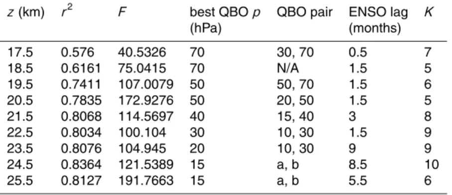
Using any of the best regression models developed in the 18.5 to 25.5 km range (Table 2), the linear trend at 18.5 km for the 1984–2012 time frame is always negative and a maximum in magnitude in the 18.5–55.5 km range (Fig. 3 extends to 25.5 km). In fact, using any of these models, the altitudes with the largest trends, listed in order of 15

increasing trend magnitude are always 19.5 km and 18.5 km. This indicates that there is a linear trend in the tropical lower stratosphere strengthening toward the tropopause, seen also in the SAGE II trend. However, at 17.5 km, the magnitude of the trend from the merged dataset is too large (not shown), inconsistent with the trends from the in-dividual satellite instruments, even considering the confidence interval of the merged 20

trend. Note that for the trends from the individual satellite datasets, we used the best regression models shown in Table 2 and, at 17.5 km, the best regression model in-cludes QBO, tropopause pressure, ENSO, linear, and constant, but not EESC, since EESC cannot be applied simultaneously with linear on the individual satellite datasets because of the high correlation of these predictors.

25

(19)

ACPD

13, 16661–16697, 2013

C. E. Sioris et al.

Title Page

Tables Figures

◭ ◮

Back Close

Full Screen / Esc

Discussion

P

a

per

|

Di

scussion

P

a

per

|

Discussion

P

a

per

|

Discussi

on

P

a

per

in a statistically significant change in the linear trend magnitude. This discrepancy in trends at 17.5 km likely results from the small sample size of available months of over-lap (N=12), relative to N=24 at most altitudes. The large standard deviation of the anomaly bias (Fig. 1), which is largest among all stratospheric altitudes at 17.5 km, may be partly due to the small sample size. Furthermore, including an indicator func-5

tion (1 for OSIRIS time frame, 0 for pre-OSIRIS time frame) into the best regression model at each altitude (see Table 2) indicates that the indicator function has the largest signal and smallest relative uncertainty at 17.5 km. This test points to an artificial step between OSIRIS and SAGE II time series, likely due to an imprecise anomaly bias correction, which likely stems partly from the seasonal biases in OSIRIS. Thus, we 10

present the trend above 18 km, where the indicator function signal is weaker and the three linear trends (SAGE II, OSIRIS, merged) are consistent within the uncertainty of the merged trend.

Figure 3 shows our best estimate for the decadal trend (1984–2012) at 18.5 km is −6.5 % (95 % CI:−8.4 to−4.7 %). In order to verify the magnitude of the linear trend, 15

we can compare our linear trend profile using only SAGE II data with that determined by Forster et al. (2007) and Randel and Wu (2007) for a very similar latitude band. At 18.5 km, their decadal trends are∼ −7.5 % and∼ −5.7 % respectively. The magnitude of our SAGE II linear trend (1984–2005) at 18.5 km is (−3.3 ± 3.6) %/decade. Our 95 % CI is very large here since the SAGE II time series is shorter and sparser than the 20

merged one. At 19.5 km, Forster et al. (2007) and Randel and Wu (2007) show decadal trends of∼ −6.5 % and∼ −3.8 %, and we find (−3.9±2.5) %/decade, in agreement with Randel and Wu (2007). There is consistency on the shape of our trend profile in the 18.5–25.5 km range (Fig. 3) with these recent studies.

Figure 3 also shows the trends from OSIRIS, which are highly uncertain (i.e. 95 % CIs 25

(20)

ACPD

13, 16661–16697, 2013

C. E. Sioris et al.

Title Page

Tables Figures

◭ ◮

Back Close

Full Screen / Esc

Discussion

P

a

per

|

Di

scussion

P

a

per

|

Discussion

P

a

per

|

Discussi

on

P

a

per

|

The 95 % CIs on the linear trend for the merged dataset are comparable to the vari-ability in the linear trend due to choice of model terms, indicating that wisely choosing these explanatory variables can clearly reduce the overall error budget on the linear trend. However, at 25.5 km, ozone variability is explained almost entirely by the QBO as its signal is an order of magnitude stronger than that from any other predictor (Ta-5

ble 2), and thus the linear trend is not sensitive to the other regression model terms. The linear trend is not sensitive to the QBO pair because of the short period of its cycles. At each altitude, the best estimate of the linear trend for the merged dataset falls within the range of linear trends predicted by applicable best models developed for other altitudes (see Fig. 3 caption), providing confidence in the method. The merging 10

of OSIRIS and SAGE II datasets yields much smaller linear trend uncertainties than SAGE II alone. The merging allows for the detection of a statistically significant trend at 18.5 km, not found with SAGE II alone. The linear trend from the merged dataset and the individual datasets are in agreement at all altitudes, except at 21.5 km and 24.5 km, where the OSIRIS trend values are outliers (Fig. 3). The general agreement 15

is expected if the linear trend in ozone is driven by greenhouse gas increases, since the trend in e.g. CO₂has not changed in the last three decades.

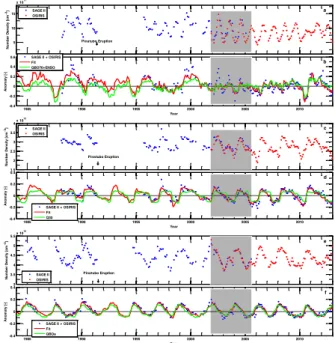
Next, we discuss the ozone variations attributable to various predictors and revisit the sensitivity of the solar term to the final linear trend estimate in Fig. 3. At 17.5– 18.5 km, the seasonal variations in ozone number density are very large yet can vary 20

from year to year (Fig. 4a). This is particularly obvious when looking at the OSIRIS time frame where there are fewer data gaps and comparing the strong annual cycles of 2002–2004 to subsequent years. Variance of this sort is di_fficult to remove by de-seasonalization or by regression modelling (Fig. 4b) even if a seasonal trend had been included. Understanding what controls the year-to-year variability of the seasonal cycle 25

(21)

ACPD

13, 16661–16697, 2013

C. E. Sioris et al.

Title Page

Tables Figures

◭ ◮

Back Close

Full Screen / Esc

Discussion

P

a

per

|

Di

scussion

P

a

per

|

Discussion

P

a

per

|

Discussi

on

P

a

per

improved version of the OSIRIS ozone retrieval becomes available. Note that there is good agreement on the magnitude of the seasonal cycle between the two instruments during the overlap period (Fig. 4a).

After deseasonalizing the ozone data records, the important predictors of ozone vari-ability throughout the tropical lower stratosphere (LS) are QBO, ENSO, tropopause 5

pressure and the linear trend, which are all statistically significant at all altitudes in the 18.5–24.5 km range (Table 2), and only tropopause pressure and the linear trend are not statistically significant at 25.5 km. At 18.5 km, the ozone response to ENSO is (−5.8±1.5) %. The ozone response and its uncertainty are calculated as the standard deviation of the basis function multiplied by its fitting coefficient or fitting coefficient 10

95 % CI, respectively. ENSO explains almost as much of the variance as the QBO at 18.5 km and more than the linear term in the 18.5–21.5 km range. The major La Nina events of 1988–1989 and 1999–2000 (Randel and Thompson, 2011) appear as positive ozone anomalies in Fig. 4b, and the latter one was also observed by HALOE (Solomon et al., 2012). The lag, much like the amplitude of ENSO, is increasingly im-15

portant at the tropopause (17.5 km), where a half-month error can reduce both the unexplained portion of the ozone variance and the linear trend uncertainty by ∼1 % (relative), whereas above 19 km, ther2reduction is never>0.35 %.

Table 2 shows that the fitted amplitudes of ENSO, tropopause pressure and the linear trend all peak at 18.5 km. They decrease strongly with increasing altitude, whereas the 20

amplitude of the QBO signal in ozone, which peaks at 19.5 km, only decreases by 30 % up to 25.5 km. ENSO and tropopause pressure signals exponentially decay with scale heights of∼4 km.

In the 18–26 km range, QBO is the key predictor of ozone variability (see Fig. 4d, f). The best single QBO pressure at an altitude tends to correspond approximately to the 25

(22)

ACPD

13, 16661–16697, 2013

C. E. Sioris et al.

Title Page

Tables Figures

◭ ◮

Back Close

Full Screen / Esc

Discussion

P

a

per

|

Di

scussion

P

a

per

|

Discussion

P

a

per

|

Discussi

on

P

a

per

|

50 hPa however it is not a statistically significant term as the QBO signal in ozone is almost entirely captured by the local QBO time series (i.e. at 70 hPa). At 19.5 km, the QBO pair is 50 and 70 hPa, but the relative contribution from the 50 hPa time series increases. At 20.5 km, which corresponds to a tropical pressure of slightly<50 hPa, the 70 hPa time series is no longer useful, and again the most orthogonal time series 5

to 50 hPa is the complementary one: 20 hPa. The complementary QBO term between 21.5 and 23.5 km tends to also be at a lower pressure which is orthogonal to the QBO time series at the local pressure. Above 22 km, there is also a tendency for the single best QBO pressure to be slightly lower than the local pressure (i.e. higher altitude). These tendencies toward lower pressures likely arise from the downward propagation 10

of the QBO. The “orthogonal” complementary QBO pressures tend to have a lag of 1/4 of the QBO period relative to the single best QBO pressure and thus provide maximum independent information and also account for any lag in the ozone response to the local QBO signal (Witte et al., 2008). These pairs of QBO basis functions act similarly to the orthogonalized QBO basis functions of Randel and Wu (2007). In fact, the correlation 15

between 10 and 30 hPa, and between 30 and 70 hPa is weaker than the correlation be-tween the two orthogonalized QBO basis functions. Figure 4d and f also illustrate that the QBO signature is altitude-dependent and any attempt to fit the QBO signal with time series at a single inappropriate pressure (even with a lag) (e.g. Cunnold et al., 2000; Bodeker et al., 2013) will fail to capture the altitude dependence of the QBO signal. 20

For example, the QBO signal in ozone exhibits sharp temporal changes at the times of extreme amplitude at 24.5 km whereas at 22.5 km, it has much more of a square-wave character (see also Dunkerton and Delisi, 1985). This is particularly evident during the two QBO cycles in the 1998 to 2003 time frame. This finding extends beyond ozone to understanding variations of other applicable trace gases (e.g. water vapour). Thus, it is 25

(23)

ACPD

13, 16661–16697, 2013

C. E. Sioris et al.

Title Page

Tables Figures

◭ ◮

Back Close

Full Screen / Esc

Discussion

P

a

per

|

Di

scussion

P

a

per

|

Discussion

P

a

per

|

Discussi

on

P

a

per

more variance than the two orthogonalized QBO basis functions. This method of ac-counting for the altitude dependence of the QBO in vertically-resolved ozone time se-ries analysis allows forr2=0.74 using only SAGE II data at 18.5 km in contrast to≤0.4 found by Randel and Wu (2007) (see also Table 1 for altitude-dependence ofr2using the merged dataset) and improves the linear trend uncertainty. However, at higher alti-5

tudes (24.5–25.5 km), the use of orthogonalized QBO basis functions (Randel and Wu, 2007) considerably improves the fit of the regression over any pair of QBO pressures. This is expected since air at 24–26 km has a much broader range of ages than air below 21 km (which has highly peaked age spectrum and is thus represented well by the QBO signature at a single appropriate pressure or two enveloping pressure levels). 10

Given the possible correlation of time series at adjacent QBO pressures, which occurs at 19.5 km (Table 1), where the best pair is 50 and 70 hPa and the correlation coef-ficient between these QBO time series is 0.64, we verified using an alternate, more orthogonal pair (30 and 70 hPa) that there is no statistically significant change in the magnitude of the linear trend, but a larger linear trend uncertainty using the latter QBO 15

pair. The semi-annual harmonic of the QBO is a weaker signal than the annual one as expected for tropical lower stratosphere (Dunkerton, 1990).

Total ozone is well known to be correlated with tropopause pressure, even over large spatial scales, particularly near 30◦S in austral summer, whereas at the equator, the correlation is much weaker (Schubert and Munteanu, 1988). Stratospheric ozone mix-20

ing ratio also has been shown to correlate with tropopause height at southern mid-latitudes (Bodeker et al., 1998). We are able to detect a coherent tropopause pressure signal in the ozone anomaly time series that has a maximum response of (4.5±2.1) % at 17.5 km and decays exponentially up to 25.5 km. The linear trend magnitude does not change in a statistically significant way with tropopause pressure included in the 25

final regression model at any altitude but the trend uncertainty profile is reduced con-siderably.

(24)

ACPD

13, 16661–16697, 2013

C. E. Sioris et al.

Title Page

Tables Figures

◭ ◮

Back Close

Full Screen / Esc

Discussion

P

a

per

|

Di

scussion

P

a

per

|

Discussion

P

a

per

|

Discussi

on

P

a

per

|

cycles. Between 17.5 and 20.5 km, including the solar term worsens the linear trend uncertainty and biases the linear trend, although the magnitude of the solar fitting co-efficient is larger than its 95 % CI. For all of the other predictors, if their fitting coefficient was larger than its 95 % CI, the inclusion of that predictor tended to improve the linear trend uncertainty as well. The special behaviour of the solar term relates to its number 5

of cycles in the merged data record being small and non-integer. Our trend-oriented stepwise regression modelling is different from regression models targeting an over-all understanding of sources of variability (e.g. Randel and Wu, 2007). We also find anomalous solar signals below 21 km if we duplicate their method. A statistically sig-nificant positive ozone response arises (+0.4 %) at 25.5 km. Per 100 units of 10.7 cm 10

radio solar flux, the change in ozone is (0.88±0.79) %, in agreement with the ∼1 % found by Randel and Wu (2007) in a pocket of statistically significant solar signal near 25 km using SAGE II data at low latitudes. Similarly, a statistically significant 1 % re-sponse from solar minimum to solar maximum was also found by Soukharev and Hood (2006) in a narrow vertical range near 28 km at low latitudes and later confirmed with 15

improved regression modelling (Hood et al., 2010).

4 Conclusions

We have shown that anomaly biases between OSIRIS and SAGE II in the overlap period (2001–2005) are small (<2 %) when each dataset is deseasonalized separately. Comparing with the only other linear-trend study in the tropical lower stratosphere 20

using SAGE II merged with more recent data, Randel and Thompson (2011) found statistically significant negative trends at 22.5 and 20.5 km (but not statistically signifi-cant at 24.5 km) in a 20◦N–20◦S band in the 1984 to 2009 period using SAGE II plus ozonesondes. Our results are quite similar to those of Randel and Thompson (2011) with a statistically significant negative trend in the 17.5 to 24.5 km range but not statis-25

(25)

ACPD

13, 16661–16697, 2013

C. E. Sioris et al.

Title Page

Tables Figures

◭ ◮

Back Close

Full Screen / Esc

Discussion

P

a

per

|

Di

scussion

P

a

per

|

Discussion

P

a

per

|

Discussi

on

P

a

per

Using SAGE II data only, we found that the harmonic of the linear trend (seasonal trend) and the same harmonic of a constant (seasonal cycle) are never statistically sig-nificant predictors with the same sign at any altitude (even when using a best regres-sion model specifically for SAGE II at 18.5 km). This means that there is no evidence supporting a seasonal trend. This is important given the approach taken in the desea-5

sonalization of the data using the seasonal cycle from the full data record (of each instrument). Also, when testing the seasonal trend term with the merged dataset, its amplitude was found to be weak (<3 % ozone response), and simply acted to capture any residual seasonality in the ozone anomalies from subtle changes in the phase of the seasonal cycle between instruments.

10

As discussed above, optimizing the ENSO lag can improve fitting, particularly near the tropopause (17.5 km). Using an altitude-independent lag of 2 months (Randel and Thompson, 2011) is adequate in the lowermost stratosphere (z <21 km), where the ENSO signal is strongest. Chemistry and transport models show that air at any loca-tion has a variety of ages due to transport. The frequency distribuloca-tion of ages is called 15

an age spectrum, and its central tendency can be measured using the mode. We ex-pect the observed ENSO lag profile (Table 1) to correspond to modal age of air, and indeed it compares well with other estimates in the tropical pipe (e.g. Strahan et al., 2009). Information on the mode of the age of air is important for modelling transport pathways such as horizontal mixing. The modal age of air (relative to the time of strato-20

spheric entry) is also available observationally from the transit period obtained from tape recorder plots. The noise level on the ENSO lag signal in ozone appears to be ∼0.5 month below 22 km, whereas above 22 km, the lag signal becomes increasingly less reliable for the latitude band of 0±4.5◦. Using a narrower latitude band (0±2.5◦), the ENSO lag signal appears more reliably up to 24.5 km. With either latitude band, 25

we obtain a modal age of air at 23.5 km of 9 months from the ENSO lag signal in the ozone time series in quantitative agreement with the transit period method.

(26)

ACPD

13, 16661–16697, 2013

C. E. Sioris et al.

Title Page

Tables Figures

◭ ◮

Back Close

Full Screen / Esc

Discussion

P

a

per

|

Di

scussion

P

a

per

|

Discussion

P

a

per

|

Discussi

on

P

a

per

|

measurements even as low as 18.5 km, but also by phenomena such as year-to-year seasonal cycle amplitude variations and subtle biases between the two independent datasets in the phase of seasonal cycle.

Given that the linear trend is a statistically significant basis function at all altitudes, while EESC tends to not be, our results are consistent with model results that show 5

that the driving forces behind the decadal changes in ozone in the tropical lower strato-sphere are increases in greenhouse gases and sea surface temperature (Lamarque and Solomon, 2010). Thus, in the absence of any new, dominant mechanism, decreas-ing ozone in the tropical LS can be expected for at least the current century (Waugh et al., 2009). At the tropopause, a−3 % decadal trend in ozone is expected from the 10

linear trend in tropopause pressure. In this study, near the tropical tropopause, the lin-ear trend magnitude exceeds this value. Additional contributions may arise from trends in cross-tropopause flux including overshooting convection and/or positive feedbacks involving between ozone and temperature, possibly involving non-linear increases in ozone loss as cloud surface area increases at the tropopause.

15

Acknowledgements. We thank Landon Rieger (University of Saskatchewan) for help with the SAGE II data and Fei Wu (National Center for Atmospheric Research, NCAR) for providing us with empirical orthogonal functions for modelling the quasi-biennial oscillation. We acknowl-edge Bill Randel (NCAR) for suggesting the idea of sensor-specific deseasonalization. We thank Nick Lloyd for comments regarding OSIRIS data and acknowledge his effort in

process-20

ing OSIRIS Level 0 and 1 data. We acknowledge funding from the Canadian Space Agency.

References

Adams, C., Bourassa, A. E., Bathgate, A. F., McLinden, C. A., Lloyd, N. D., Roth, C. Z., Llewellyn, E. J., Zawodny, J. M., Flittner, D. E., Manney, G. L., Daffer, W. H., and Degen-stein, D. A.: Characterization of Odin-OSIRIS ozone profiles with the SAGE II dataset, Atmos.

25

Meas. Tech., 6, 1447–1459, doi:10.5194/amt-6-1447-2013, 2013a.

(27)

mea-ACPD

13, 16661–16697, 2013

C. E. Sioris et al.

Title Page

Tables Figures

◭ ◮

Back Close

Full Screen / Esc

Discussion

P

a

per

|

Di

scussion

P

a

per

|

Discussion

P

a

per

|

Discussi

on

P

a

per

surements from 2001 to the present using MLS, GOMOS, and ozone sondes, Atmos. Meas. Tech. Discuss., 6, 3819–3857, doi:10.5194/amtd-6-3819-2013, 2013b.

Bodeker, G. E., Boyd, I. S., and Matthews, W. A.: Trends and variability in vertical ozone and temperature profiles measured by ozonesondes at Lauder, New Zealand: 1986–1996, J. Geophys. Res., 103, 28661–28681, 1998.

5

Bodeker, G. E., Hassler, B., Young, P. J., and Portmann, R. W.: A vertically resolved, global, gap-free ozone database for assessing or constraining global climate model simulations, Earth Syst. Sci. Data, 5, 31–43, doi:10.5194/essd-5-31-2013, 2013.

Bourassa, A. E., Rieger, L. A., Lloyd, N. D., and Degenstein, D. A.: Odin-OSIRIS stratospheric aerosol data product and SAGE III intercomparison, Atmos. Chem. Phys., 12, 605–614,

10

doi:10.5194/acp-12-605-2012, 2012.

Bovensmann, H., Burrows, J. P., Buchwitz, M., Frerick, J., Noël, S., and Rozanov, V. V.: SCIA-MACHY: mission objectives and measurement modes, J. Atmos. Sci., 56, 127–150, 1999. Brohede, S., Jones, A., and Jégou, F.: Internal consistency in the Odin stratospheric ozone

products, Can. J. Phys., 85, 1275–1285, 2007.

15

Chu, W. P., McCormick, M. P., Lenoble, J., Brogniez, C., and Pruvost, P.: SAGE II inversion algorithm, J. Geophys. Res., 94, 8339–8351, 1989.

Cooper, M., Martin, R. V., Sauvage, B., Boone, C. D., Walker, K. A., Bernath, P. F., McLin-den, C. A., Degenstein, D. A., Volz-Thomas, A., and Wespes, C.: Evaluation of ACE-FTS and OSIRIS Satellite retrievals of ozone and nitric acid in the tropical upper

tro-20

posphere: application to ozone production efficiency, J. Geophys. Res., 116, D12306, doi:10.1029/2010JD015056, 2011.

Cunnold, D. M., Wang, H. J., Thomason, L. W., Zawodny, J. M., Logan, J. A., and Megret-skaia, I. A.: SAGE (version 5.96) ozone trends in the lower stratosphere, J. Geophys. Res., 105, 4445–4457, 2000.

25

Damadeo, R. P., Zawodny, J. M., Thomason, L. W., and Iyer, N.: SAGE version 7.0 algorithm: application to SAGE II, Atmos. Meas. Tech. Discuss., 6, 5101–5171, doi:10.5194/amtd-6-5101-2013, 2013.

Daniel, J. S., Solomon, S., and Albrittion, D. L.: On the evaluation of halocarbon radiative forcing global warming potentials, J. Geophys. Res., 100, 1271–1285, 1995.

30