RECONSTRUCTION AND SEARCHING OZONE DATA PERIODICITIES IN SOUTHERN
BRAZIL (29ºS, 53ºW)
NIVAOR RODOLFO RIGOZO
1, MARCELO BARCELLOS DA ROSA
2, PABULO HENRIQUE
RAMPELOTTO
3, MARIZA PEREIRA DE SOUZA ECHER
4, EZEQUIEL ECHER
4, DANIEL JEAN
ROGER NORDEMANN
4, DAMARIS KIRSCH PINHEIRO
2, NELSON JORGE SCHUCH
11
Instituto Nacional de Pesquisas Espaciais, Centro Regional Sul de Pesquisas Espaciais (INPE/CRS), Santa
Maria, RS, Brasil
2
Universidade Federal de Santa Maria (UFSM), Departamento de Química, Santa Maria, RS, Brasil
3
UFSM, Departamento de Biologia, Santa Maria, RS, Brasil
4INPE, Divisão de Geofísica Espacial, São José dos Campos, SP, Brasi
l[email protected], [email protected], [email protected], [email protected],
[email protected], [email protected], [email protected], [email protected]
Received October 2010 – Accepted November 2011
ABSTRACT
Ozone plays a very important role in the nature due its characteristics as a natural ilter of ultraviolet solar radiation. Thus, it is pertinent for the scientiic community to understand all natural inluence factors involving ozone along with a large time series. In this work, a reconstruction of ozone time series obtained by Brewer spectrophotometer from 1994 to 2008 at the Southern Space Observatory (SSO) - 29ºS, 53ºW - Southern Brazil is presented. TOMS-OMI data were used to follow the days without data, where a coeficient of correlation between TOMS-OMI and Brewer is acceptable around r = 0.89. Besides, wavelet analysis to determine the temporal evolution of the frequencies and the amplitudes was applied. Moreover, wavelet analysis aiming to determine the temporal evolution of the frequencies and the amplitudes was performed. The results pointed a period of 365 days (1 yr) for the seasonal variation of ozone, of 600 days attributed for a possible QBO inluence and two periods of 2000 and other 4000 days regarding possibly to the second harmonic of the 11-year solar cycle. Keywords: Ozone, Brewer, Quasi-Biennial Oscillation, solar activity, wavelet analysis
RESUMO: RECONSTRUÇÃO E PROCURA DE PERIODICIDADES NOS DADOS DE OZONIO REGIÃO SUL DO BRASIL (29ºS, 53ºW)
O ozônio tem um papel muito importante na natureza devido as suas características como um iltro natural da radiação solar ultravioleta. Portanto, é pertinente para a comunidade cientíica compreender todos os fatores de inluência natural envolvendo ozônio ao longo das séries temporais de grande porte. Neste trabalho, uma reconstrução da série temporal do ozônio obtido pelo espectrofotômetro Brewer 1994-2008 no Observatório Espacial do Sul (29 º S, 53 º W) - Sul do Brasil é apresentado. Os dados do TOMS-OMI foram usados para completar os dias sem dados, onde um coeiciente de correlação entre TOMS-OMI e Brewer é aceitável, em torno de r=0,89. Além disso, foi aplicada a análise de ondeletas para determinar a evolução temporal das frequências e das amplitudes. Os resultados apontam um período de 365 dias (ou 1 ano) para a variação sazonal do ozônio, um período de 600 dias para uma possível inluência QBO e dois períodos, um de 2000 e outro de 4.000 dias referentes ao segundo harmônico do ciclo solar de 11 anos e 11 Ciclo de ano solar.
1. INTRODUCTION
The monitoring of ozone by different ground instruments and space-born systems results in a collection of diverse data sets that have been used to investigate ozone changes caused by natural atmospheric processes and/or chemical emissions. Estimations of ozone trends and the beginning of the recovery of the ozone layer are the high-priory research tasks that require assessment of the relation between long-term data records of different origins. Many details of the expected ozone recovery are unclear so are the possible interactions with climate change and the consequences of increasing bromine (Salby and Callaghan, 2002; Ramaswamy et al., 2001). In order to actually “see” a recovery, high quality measurements are needed for many years to come. For the early detection of signs of a recovery or of a possible worsening, a good quantitative understanding is necessary for the various natural processes, which contribute to the variation of ozone levels from year to year.
The ozone distribution itself is driven by atmospheric circulation and atmospheric temperature distribution. It is inluenced by its variability, and hence potentially affected by climate change [World Meteorological Organization (WMO), 2006].
In order to identify the key processes in the atmospheric ozone budget, satellite soundings of the atmospheric abundance of the relevant trace gases have been routinely performed since the 1970s. These satellite observations allow us to determine the total ozone column and vertical profiles of ozone in the atmosphere, from the stratosphere down into the troposphere. Thus, ground-based observations have been widely used as a validation tool for satellite data or in terms of complementation of satellite data by means of extending the tropospheric observations down to the surface, where most satellite instruments have a reduced sensitivity. This is especially important to understand the role of local and regional sources and sinks of tropospheric ozone and its precursors.
Satellite remote sensing observations are currently commonly used for the daily monitoring of the state of the global-ozone layer from regional to continental spatial scales, as well as for the investigation of the chemical and dynamical causes of ozone decline. Also, such observations are likely to be used for the monitoring of the expected future global-ozone recovery. Satellites provide a global view of the Earth’s atmospheric system over extended periods of time, with an appreciable spatial resolution allowing the detection of regional- to global-scale ozone trends. Recently, several space-based instruments have been designed for retrieving the total ozone column (TOC) from observations of backscattered solar irradiance emerging at the top of the atmosphere.
Several studies using ground based and satellite measurements have demonstrated that since the late 1970s until the early 1990s, there have been signiicant negative trends in total ozone in the middle and high-latitude regions of the two hemispheres (Harris et al., 1997, Staehelin et al., 2001). The implementation of the Montreal Protocol Ozone Layer depletors and their later amendments have created high expectations about the recovery of the total ozone toward pre 1980s concentrations as a result of the declining halogen loading in the stratosphere. Thus, Newchurch et al. (2003) reported signs of an ozone turnaround after 1996 from a statistical analysis of observations in the upper stratosphere, where ozone is mainly controlled by gas phase catalytic cycles.
Satellite instruments provide daily images of the global ozone distribution with good spatial resolution that is an important advantage over the local measurements of ground-based ozone from a sparse network. TOMS global observations have proven to be crucial to the understanding of the geographical and temporal distribution and variability of TOC (Hudson et al., 2006; Antón et al., 2008). These observations are being continued by the Ozone Monitoring Instrument aboard the NASA EOS Aura platform (Levelt et al., 2006) since October 2004.
In terms of data validation, Balis et al. (2007) showed a small negative bias of −1% and a seasonal behavior with amplitude of ±0.5% for EP-TOMS–Brewer comparisons with the corrected satellite data set, while McPeters and Labow (1996) analyzed the satellite–ground based differences as a function of satellite solar zenith angle (SZA) for Northern Hemisphere stations (25◦ N to 55◦ N) for OMI TOC data and for empirically corrected EP-TOMS TOC data. While the EP-TOMS SZA-dependent error increases to almost −3% at 70◦ SZA, OMI TOC shows no signiicant dependence on SZA. Therefore, many studies have investigated variations of ozone and as consequence temperature on interannual time scales has been observed. This includes trends (Bojkov et al., 1990; Staehelin et al., 2001), inluences from the QBO (Baldwin et al., 2001), from the 11-year solar cycle (Labitzke and van Loon, 2000; Lee and Smith, 2003), from El Ninõ/Southern Oscillation (ENSO) (Reid, 1994) or from meteorological factors (Appenzeller et al., 2000; Steinbrecht et al., 2001).
increasing tropical total ozone and adiabatically warming the tropical lower stratosphere.
Speciously addressing the atmospheric characteristics from the South of Brazil, aspects as the South Atlantic Geomagnetic Anomaly as well as the secondary ozone effects, which are lower levels of ozone from Antarctica coming yearly and normally in Spring, we proposed to reconstruct ozone time series considering the data over our region, South of South America, aiming to search periodicity signals on ozone time series. In other words, this work aimed to collaborate in the comprehension of the mechanisms driving the ozone variability in Southern Brazil.
2. DATA AND METODOLOGY
2.1 Satellite measurements
TOMS-OMI from NASA/Goddard Space Flight Center was used as our data source. The NASA TOMS series of four satellite instruments has been successfully designed and launched for measuring global TOCs since November 1978. The last TOMS instrument of this series was launched in July 1996 aboard the EP satellite. The EP-TOMS instrument measures solar irradiance and the radiance backscattered by the Earth’s atmosphere in six selected wavelength bands in the ultraviolet (UV) spectral region (between 308 and 360 nm)
2.2 Ground-Based data
The Brewer spectrophotometer works with principles similar to the Dobson instrument but has an improved optical
design and is fully automated. TOC values are obtained taking the ratio of sunlight intensities at four wavelengths between 306 and 320 nm with a resolution of 0.6 nm overcoming the spectral interference of sulfur dioxide with ozone (Kerr, 2002). A Brewer Spectrophotometer 167 installed at Southern Space Observatory – Sao Martinho da Serra – Southern Brazil, is an MKIII model with double monochromator and resolution of 0.6 nm and has been used in the monitoring of the total atmospheric ozone (O3), sulfur dioxide (SO2) columns and UV-B solar irradiance.
The days considered in our analysis were selected according to the following criteria: (i) because of Brewers data, the individual DS ozone observations are performed ive times in 3 min. The ozone standard deviations are computed on a group of ive individual DS measurements for each wavelength. Data are accepted if the standard deviation is lower than 2.5 DU; (ii) to obtain a better statistics analysis, the number of the individual DS data must be at least 35 (seven sequences of ive observations); (iii) only typical clear sky days at solar zenith angles below 65 were considered in the calculation of ozone.
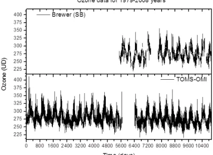
The interval of ozone Brewer data was between 1994 - 2008, while for TOMS-OMI the period was 1979 - 2008. Figure 1 presents a generic proile with gaps of Brewer and TOMS data.
2.3 Methodology
2.3.1 Deinition of error
A linear regression analysis was performed using the Brewer x TOMS-OMI data considering 1994-2008. Regression
coeficients, coeficients of correlation (R2) and the root mean square errors (RMSE) were calculated and the mean bias error (MBE) comparing Brewer x TOMS-OMI measurements was calculated. These parameters are obtained by the following expression:
where N is the number of data pairs Brewer- TOMS.
2.3.2 Savitzky-Golay smoothing
One way of smoothing data and suppressing disturbances is to use a ilter, and replace each data value Ii, i =1,..., N by a linear combination of nearby values in a window:
In the simplest case, referred to as a moving average, the weights are cj=1/(2n+1) and the data value Ii is replaced by the average of the values in the window. The moving average method preserves the area and mean position of a seasonal peak, but alters both the width and height. The latter properties can be preserved by approximating the underlying data value, not by the average in the window, but with the value obtained from a least-squares it to a polynomial. For each data value Ii; We it a we it a polynomial of ifth order:
to all 2n+1 points in the moving window and replace the value Ii with the value of the polynomial at position ti : The procedure above is commonly referred to as an Savitzky–Golay ilter (Press et al., 1995, Jönsson and Eklundh, 2004).
The Savitzky-Golay ilter method essentially performs a local polynomial regression to determine the smoothed value for each data point. This method is superior to adjacent averaging because it tends to preserve features of the data such as peak height and width, which are usually ‘washed out’ by adjacent averaging (Press et al., 1995).
2.3.3 Wavelet analysis
In terms of mathematical tool, we drive our study using wavelet transform, which is a powerful tool for non stationary signal analysis and permits to identify the main periodicities
N TOMS TOMS Brewer RMSE N i
∑
= − = 1 2 * 100 (%) (1)∑
= − = N I TOMS TOMS Brewer N MBE 1 100 (%) (2)∑
− = + n n j i j jI c (3) 5 6 4 5 3 4 2 3 2 1 )(t c ct ct ct ct ct
f = + + + + +
(4)
in a time series and their evolution (Kumar and Foufoula-Georgiou, 1997; Torrence and Compo, 1998; Percival and Walden, 2000). The wavelet transform of a series of discrete data is deined as the convolution between the series and a scaled and translated version of the wavelet function chosen. By varying the wavelet time scale and translating the scaled versions of the wavelet, it is possible to build a graph showing the amplitudes versus frequency (or scale) and how they vary with time.
Herein, we used the complex Morlet wavelet function, which consists of a plane wave modulated by a Gaussian function: 0
( )
1/4 /22 0h h w
π h
y = − −
e
ei , where wo is the
non-dimensional frequency and h a nondimensional “time” parameter. Let us assume that the time series, xn, has equal time spacing Dt, with n =0,..., N-1 . To be “admissible” as a wavelet, this function must have zero mean and be localized in both time and frequency space (Farge, 1992). Therefore, the continuous wavelet transform of xn is deined as the convolution of xn with a scaled and translated version of y0 (h):
where (*) indicates the complex conjugate and
s
the wavelet scale. The technique allows to construct a picture showing the variation of amplitude in time and scale (Torrence and Compo, 1998).If a vertical slice through a wavelet plot is a measure of the local spectrum, then the time-averaged wavelet spectrum over a certain period is when the average is over all the local wavelet spectra, which gives the global wavelet spectrum (Torrence and Compo, 1998):
Percival (1995) shows that the global wavelet spectrum provides an unbiased and consistent estimation of the true power spectrum of a time series. Finally, it has been suggested that the global wavelet spectrum could provide a useful measure of the background spectrum, against which peaks in the local wavelet spectra could be tested (Kestin et al. 1998).
In addition, the cross-wavelet analysis indicates whether exists or not a correspondence between detected cycles from independent time series, obtained for the same time base. If two time series X and Y are given, with respective wavelet transforms WnX
( )
s and WnY( )
s , one can deine the cross-wavelet spectrum as WnYX( )
s =WnX( )
s[
WnY*( )
s]
, where WnY*( )
s is the complex conjugate of WnY( )
s . The cross-wavelet spectrum is complex, and hence one can deine the cross-wavelet power as( )
2s
WsXY (Torrence and Compo, 1998).
( )
∑
−(
)
=
− D
= 1 0 ' ' ' * N n n n s t n n x s W y (5) 2 1 0 2( ) 1
∑
− ( )3. RESULTS AND DISCUSSION
Before the reconstruction of the ozone Brewer data, a mathematical difference between TOMS-OMI and Brewer was performed (Figure 2), where the data with a statistical difference greater than 1s is discarded. The correlation between the TOMS-OMI and Brewer data was from r = 0.89 (Figure 3) to r = 0.93, when we used this criterion. Indeed, only after these data adjust we started the reconstruction of the ozone Brewer data in two ways, each subdivided in two supplementary steps:
• First way: 1- We obtained a linear regression between the TOMS-OMI and Brewer data, where the coeficient of correlation is r = 0.93; 2- The gaps that could not be obtained by the linear regression were interpolated using
Figure 2 – Ozone difference between TOMS and Brewer Southern Brazil.
the Savitzky-Golay ilter method (Press et al., 1995, Jönsson and Eklundh, 2004).
• Second way: 1- As a high correlation between the TOMS-OMI and Brewer data was observed, we completed the missing Brewer data with TOMS data; 2- The gaps that could not be obtained by the TOMS-OMI data were interpolated using the Savitzky-Golay ilter method (Press et al., 1995, Jönsson and Eklundh, 2004).
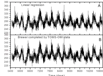
The ozone Brewer reconstructed “irst way” is presented in Figure 4a and “second way” in Figure 4b. The irst way reconstructed shows a mean of 274.7±19.6 for Brewer and 273.9±20.1 in terms of ozone fro TOMS. To investigate the proportionality and similarity of the ground-based and satellite-based observations, the Brewer and OMI total ozone column
data are itted using a linear regression. Statistical parameters obtained are shown in Table 1. The correlation between TOMS ozone observations and Brewer measurements is signiicantly high. The R2 values higher than 0.78 are indicative of the ground-based and satellite-based data sets showing a similar behavior. The statistical analysis renders slopes very close to unity. The scatterplot presented in Figure 3 between satellite and ground-based data for the Southern Brazil (29ºS, 53ºW) data set reveal a high degree of proportionality. It can be seen that the RMSE values and uncertainty of MBE parameters are signiicantly lower. These reveal a high degree of proportionality with a notably small spread (RMSE smaller than 4%). This reveals the presence of a bias with a small statistical spread. The uncertainty of MAB parameters is lower than 1%, indicating the statistical signiicance of the reported values. Bhartia and Wellemeyer (2002) reported that the relative uncertainty of OMI-TOMS ozone data is around 2% for solar zenith angles lower than 70 degrees. Therefore, apparently a signiicant difference between the reconstructed ozone data is considered insigniicant.
The wavelet spectra show negligible differences between the two reconstructed time series. This situation is most clearly observed when we consider the cross-wavelet spectrum between the two way ozone reconstruction data (Figure 5), where the
same period variation in time is observed as in wavelet spectra for ozone Brewer reconstructed time series (Figure 4).
This signal indicates a possible seasonal variation of the ozone. Also, the existence of other periods was observed between 530-900 days being more persistent in two time series, as well as approximately between 5480-7758 and 8858-10958 days. In this case, the periodicities come from a possible QBO inluence on ozone in Southern Brazil.
It is observed that a period variation exists with the time of ~2000 days, which is more persistent to time interval of 5480-8858 days in terms of long trends. In this case, we assign these frequencies as a possible inluence of the second harmonic of the 11-year solar cycle regarding ozone in Southern Brazil.
The wavelet spectrum of reconstructed ozone from time series indicates the strongest feature and a persistent signal near 365-days (Figure 5). This signal indicates a possible seasonal variation of the ozone. Also, the existence of other periods was observed between 530-900 days being more persistent in two time series, as well as approximately between 5480-7758 and 8858-10958 days. In this case, the periodicities come from a possible QBO inluence on ozone in Southern Brazil. Hood and McCornack (1992) reported have found the QBO signal in their studies about components of interannual ozone change based on NIMBUS 7 TOMS data to 65oN-65oS. Sych et al. (2005), also, reported this signal of 2.5 years of QBO inluence on ozone to 10o S latitude, in yours studying about the periodic spatial–temporal characteristics variations of the total ozone content. It is observed that a period variation exists with the time of ~2000 days, which is more persistent to time interval of Figure 4 – Ozone Brewer reconstructed from Southern Brazil (1994-2008) by: First way, linear regression between the TOMS-OMI and Brewer data (a); Second way, Brewer data completed by TOMS-OMI data (b).
N Slope R2 RMSE(%) MBE(%)
2641 0.89 0.79 3,6 0,9
Figure 5 – Ozone Brewer Reconstructed by linear regression wavelet spectrum (a). Ozone Brewer Reconstructed by completed TOMS-OMI data
wavelet spectrum (b). The cone of inluence (parabolic curve, white line), and signiicance levels contour for 95%. At right the legend indicates
Amplitude spectra scale in grayscale. Y-axis is the scale (period) in days, X-axis is the time, in days. 5480-8858 days in terms of long trends. In this case, we assign
these frequencies as a possible inluence of the second harmonic of the 11-year solar cycle regarding ozone in Southern Brazil. The wavelet spectra show negligible differences between the two reconstructed time series. This situation is most clearly observed when we consider the cross-wavelet spectrum between the two ways ozone reconstruction data (Figure 6), where the same period variation in time is observed as in wavelet spectra in both ozone Brewer reconstructed time series (Figure 5).
The data of the ozone from TOMS-OMI presents a long time series in comparison with our Brewer data. Therefore,
we used the irst one in the reconstruction of ozone Brewer
data considering the very good correlation factor obtained from the linear regression between the two time series. The reconstructed ozone Brewer data for our region, 29ºS, 53ºW, is presented in Figure 7a. The wavelet spectrum of new ozone Brewer reconstructed time series in Southern Brazil (Figure 7b) shows that the periodicities (seasonal, QBO and second harmonic of the 11-yr solar cycle variations) found in Figures 5a and 5b remain in the past 1-5400 days. Thus, increasing the time series it is possible to observe a representative periodicity of the second harmonic of the 11-yr solar activity (~2000 days)
Figure 6 – The cross-wavelet spectrum for to two ways for both the ozone Brewer reconstruction (a) and Global wavelet spectrum (b). The cone of
inluence (parabolic curve, white line), and signiicance levels contour for 95%. At right the legend indicates Amplitude spectra scale in grayscale.
as a strong feature. Furthermore, a persistent time for the 1500-8258 days (Figure 7b) has also been observed, in which it is also possible to show a periodicity of ~4000 days (Figure 7b) and that is related with a possible inluence of the 11-yr solar cycle in ozone in Southern Brazil. This results in agreement with Hood and McCornack (1992) that reported to have found the of solar cycle (10-11 years) inluence on ozone change based on NIMBUS 7 TOMS data to 65oN-65oS. So who, Sych et al. (2005), also, reported this signal of 11.0 years of solar cycle inluence on ozone to 10o S latitude, and Soukharev and Hood (2006) have found a response of the solar cycle variation of stratospheric ozone in the two hemispheres.
4. CONCLUSION
In this work ozone Brewer time series for Southern Brazil were reconstructed and wavelet analysis was applied. We have found the following periodicities that inluence the ozone: (i) A seasonal variation with periodicity of ~365 days; (ii) The QBO phenomenon with periodicity of ~530-900 days; (iii) The second harmonic of the 11-yr solar cycle with periodicity of ~2000 days; and (iv) The 11-yr solar cycle with periodicity of ~4000 days.
Therefore, we contributed with an overview and proile of ozone data on our region (29ºS, 53ºW) and presented some aspects involving the ozone periodicities in the South of Brazil. We understand further studies are necessary to obtain more precise information on the current weather conditions in South
Figure 7 – Ozone Brewer Reconstructed time series by linear regression (a). Wavelet spectrum (b) and Global wavelet spectrum (c). The cone of
inluence (parabolic curve, white line), and signiicance levels contour for 95%. At right the legend indicates Amplitude spectra scale in grayscale.
Y-axis is the scale (period) in days, X-axis is the time, in days.
America as a whole. Thus, we also intended with this work to collaborate as source for mathematical models that address global climate changes and their direct or indirect effects on the ozone behavior and global dynamic.
5. ACKNOWLEDGMENTS
Authors would like to thanks for support granted to this research: N. R. Rigozo - CNPq (APQ 470252/2009-0, 470455/2010-1 and research productivity, 301033/2009-9) and FAPERGS (APQ 1013273); M.P Souza Echer - CNPq (151609/2009-8); CNPQ/PQ (300211/2008-2) e FAPESP (2007/52533-1); A. Prestes FAPESP - (2009/02907-8).
6. REFERENCES
ANDREWS, D. G.; HOLTON, J. R.; LEOVY, C. B. Middle Atmosphere Dynamics. San Diego: Academic, 1987. ANTÓN, M.; LOYOLA, D.; NAVASCU´ES, B.; VALKS, P.
Comparison of GOME total ozone column data with ground data from the Spanish Brewer spectroradiometers. Annales Geophysicae., v. 26, p. 401– 412, 2008.
APPENZELLER, C.; WEISS, A. K.; ST AHELIN, J. North Atlantic Oscillation modulates total ozone winter trends. Geophysical Research Letters, v. 27, p. 1134–1138, 2000. BALDWIN, M. P.; GRAY, L. J.; DUNKERTON, T. J.;
HOLTON, J. R.; ALEXANDER, M. J.; HIROTA, I.; HORINOUCHI, T.; JONES, D. B. A.; KINNERSLEY, J. S.; MARQUARDT, C.; TAKAHASHI, M. The Quasi-Biennial Oscillation. Reviews of Geophysics, v. 39, p. 179–229, 2001.
BALIS, D.; KROON, M.; KOUKOULI, M. E.; BRINKSMA, E. J.; LABOW, G.; VEEFKIND, J. P.; MCPETERS, R. D. Validation of Ozone Monitoring Instrument total ozone column measurements using Brewer and Dobson spectrophotometer ground-based observations. Journal
of Geophysical Research, v. 112, D24S46, 2007, doi:10.1029/2007JD008796.
BHARTIA, P. K.; C. WELLEMEYER. TOMS-V8 total O3 algorithm, in OMI Algorithm Theoretical Basis Document, vol. II, OMI Ozone Products, edited by P. K. Bhartia, p. 15– 31, NASA Goddard Space Flight Cent., Greenbelt, Md., 2002. (Available at http://eospso.gsfc.nasa.gov/ eos_homepage/for_scientists/atbd/index.php)
BOJKOV, R. D.; BISHOP, L.; HILL, W. J.; REINSEL, G. C.; TIAO, G. C. A statistic trend analysis of revised Dobson total ozone data over the Northern Hemisphere. Journal of Geophysical Research, v. 95, p. 9785–9807, 1990. FARGE, M. Wavelet transforms and their applications to
turbulence. Annual Reviews Fluids Mechanics, v. 24, p. 395–457, 1992.
HARRIS, N. R. P., et al. Trends in stratospheric and free tropospheric ozone. Journal of Geophysical Research, v. 102, p. 1571–1590, 1997, doi:10.1029/96JD02440. HOOD, L. L.; MCCORMACK, J. P. Components of
interannual ozone change based on NIMBUS 7 TOMS data. Geophysical Research Letters, v. 19, p. 2309-2312, 1992. HUDSON, R. D.; ANDRADE, M. F.; FOLLETTE, M. B.;
FROLOV, A. D. The total ozone field separated into meteorological regimes. Part II: Northern Hemisphere midlatitude total ozone trends. Atmospheric Chemistry and Physics, v. 6, p. 5183–5191, 2006.
JÖNSON, P.; EKLUNDH, L. TIMESAT—a program for analyzing time-series of satellite sensor data. Computers & Geosciences, v. 30, p. 833–845, 2004.
KERR, J. B. New methodology for deriving total ozone and other atmospheric variables from Brewer spectrophotometer direct sun spectra. Journal of Geophysical Research, 107(D23), 4731, 2002, doi:10.1029/2001JD001227. KESTIN, T. S.; KAROLY, D. J.; YANO, J.-I.; RAYNER, N.
A. Time– frequency variability of ENSO and stochastic simulations. Journal of Climate, v. 11, p. 2258–2272, 1998. KUMAR, P.; FOUFOULA-GEORGIOU, E. Wavelet Analysis
for geophysical applications. Reviews of Geophysics, v. 35, p. 385-412, 1997.
LABITZKE, K.; VAN LOON, H. The QBO effect on the
solar signal in the global stratosphere in the winter of the Northern Hemisphere. Journal of Atmospheric and Solar-Terrestrial Physics, v. 62, p. 621–628, 2000.
LEE, H.; SMITH, A. K. Simulation of the combined effects of solar cycle, quasi-biennial oscillation, and volcanic forcing on stratospheric ozone changes in recent decades.
Journal of Geophysical Research, v. 108, ACH 4, 2003. doi:10.1029/2001JD001503.
LEVELT, P. F., E. HILSENRATH, G. W. LEPPELMEIER, G. H. J. VAN DEN OORD, P. K. BHARTIA, J. TAMMINEN, J. F. DE HAAN, AND J. P. VEEFKIND. Science objectives of the Ozone Monitoring Instrument. IEEE Transactions on Geoscience & Remote Sensing, v. 44, p. 1199– 1208, 2006. doi:10.1109/TGRS.2006.872336.
MCPETERS, R. D.; LABOW, G. J. An assessment of the accuracy of 14.5 years of Nimbus 7 TOMS version 7 ozone data by comparison with the Dobson network. Geophysical Research Letters, v. 23, p. 3695 – 3698, 1996, doi:10.1029/96GL03539.
NEWCHURCH, M.; YANG, E.-S.; CUNNOLD, D. M.; REINSEL, G. C.; ZAWODNY, J. M.; RUSSELL III, J. M. Evidence for slowdown in stratospheric ozone loss: First stage of ozone recovery. Journal of Geophysical Research, v. 108, p. 4507, 2003, doi:10.1029/2003JD003471. PERCIVAL, D. P. On estimation of the wavelet variance.
Biometrika, v. 82, p. 619–631, 1995.
PERCIVAL, D. B.; WALDEN, A. T. Wavelet Methods for Time Series Analysis. Cambridge: Cambridge University Press, 2000.
PRESS, W. et al. Numerical Recipes in C. Cambridge University Press, Second Edition, 1995.
RAMASWAMY, V.; CHANIN, M. L.; ANGELL, J.; BARNETT, J.; GAFFEN, D.; GELMAN, M.; KECKHUT, P.; KOSHELKOV, Y.; LABITZKE, K.; LIN, J. J. R.; O‘NEIL, A.; NASH, J.; RANDEL, W.; ROOD, R.; SHIOTANI, M.; SWINBANK, R.; SHINE, K. Stratospheric temperature trends: observations and model simulations. Reviews of Geophysics, v. 39, p. 71–122, 2001.
REID, G. C. Seasonal and interannual temperature variations in the tropical stratosphere. Journal of Geophysical Research, v. 99, p. 18923–18932, 1994.
SALBY, M. L.; CALLAGHAN, P. F. Interannual changes of the stratospheric circulation: relationship to ozone and tropospheric structure. Journal of Climate, v. 24, p. 3673–3685, 2002.
SOUKHAREV, B. E.; HOOD, L. L. Solar cycle variation of stratospheric ozone: Multiple regression analysis of longterm satellite data sets and comparisons with models.
STAEHELIN, J.; HARRIS, N. R. P.; APPENZELLER, C.; EBERHARD, J. Ozone trends: A review. Reviews of Geophysics, v. 39, p. 231–290, 2001.
STEINBRECHT, W.; CLAUDE, H.; K¨OHLER, U.; WINKLER, P. Interannual changes of total ozone and Northern Hemisphere circulation patterns. Geophysical Research Letters, v. 28, p. 1191–1194, 2001.
SYCH, R.A.; MATAFONOV, K.; BELINSKAYA, A.JU.; FERREIRA, J. The periodic spatial–temporal characteristics variations of the total ozone content. Journal of Atmospheric and Solar-Terrestrial Physics, v. 67, p. 1779–1785, 2005
TORRENCE, C.; COMPO, G. P. A Practical Guide to Wavelet Analysis. Bulletin of the American Meteorological Society, v. 79, p. 61-78, 1998.
WORLD METEOROLOGICAL ORGANIZATION. Scientiic