Real-Dollar Exchange Rate
∗
Frederico Pechir Gomes
†
, Marcelo Yoshio Takami
‡
, Vinicius Ratton
Brandi
§
Contents: 1. Introduction; 2. Data Description; 3. Informational Content and Forecasting Accuracy; 4. Signaling for Tail Events; 5. Concluding Remarks;
Keywords:Informational Content; Predictive Power; Early Warning.
JEL Code:D40; F31; G14.
A previsibilidade das distribuições de preços de ativos financeiros con-siste em tema relevante tanto na literatura de risco como de apreçamento de ativos. Interesse especial reside na investigação acerca das probabil-idades dos eventos de cauda, cujas realizações apresentam impacto de maior severidade comparativamente ao previsto pela distribuição Normal. Este trabalho tem como objetivo verificar se as volatilidades implícitas de opções de dólar detêm conteúdo informacional e poder preditivo em re-lação a retornos de grande magnitude. Nossos resultados sugerem que es-sas expectativas de mercado, de fato, carregam informação relevante sobre retornos futuros, além de conter poder preditivo significativo.
Price distributions forecast has become a relevant subject for risk and pric-ing literature. Special concern resides on tail probabilities, which usually present more severe observations than Normal distributions would predict. This work aims to verify if the volatility implied in real-dollar options contains useful information about unexpected large-magnitude returns. Implied volatility is also checked as a predictor for realized volatility. Our results indicate that im-plied volatilities provide useful information on unusual returns and also work as a good predictor for observed volatility. Moreover, we implement an early-warning system and implied volatilities seem to signalize large-magnitude re-turns.
∗The authors would like to thank the anonymous referee for his/her valuable comments. Needless to say, any remaining errors
are ours. The views expressed in this paper are those of the authors and do not necessarily reflect those of the Banco Central do Brasil.
†Banco Central do Brasil. E-mail:[email protected]
‡Banco Central do Brasil. E-mail:[email protected]
1. INTRODUCTION
Academics, regulators and market players all agree on the benefits from a stable financial system, capable of recognizing, measuring and controlling financial risks. As Pownall and Koedijk (1999) point out, several regulatory changes have been recently put into practice worldwide in order to achieve this goal. Their purpose is to outline the advantages associated with the use of risk management tools in financial systems, reducing the potential damages originated by banking crises and systemic shocks. The authors divide these regulatory changes in two categories: the minimum capital requirements for financial institutions, recommended by the Basel Committee,1 and the dissemination of risk culture
among market participants, including the adoption of the widespread Value-at-Risk technique as a risk management tool.
Nevertheless, banking crises observed in recent years indicate that risk management tools were not able to assess the real magnitude of the risks present in turbulent periods. As stated by Blejer and Schumacher (1998), this might be related to the fact that most of the risk models were developed under naïve modeling assumptions, such as the assumption of the normality of asset returns distribution. It is well known, however, that fat-tailness consists on a stylized fact of financial time series distributions. As a consequence, the probability of a negative result may be underestimated in the tail, where accuracy should be even more demanded, due to higher severity of the corresponding events.
The relevant issue is, therefore, how to overcome those drawbacks, in a way that extreme move-ments could be better modeled and tail bias avoided. Among the several techniques available, it is worth mentioning Stress Testing, which examines the effects on portfolios of huge and unusual move-ments (high severity and low frequency) in financial variables and is often dealt with the use of the results from the Extreme Value Theory (EVT). In this regard, it is worth mentioning the development of methodologies applied to the anticipation of crises and to the search for early warning signals is a fast-growing field of study.
In general, those techniques are focused on the analysis of macroeconomic variables. Berg and Pattillo (1998), Frankel and Rose (1996) and Kaminsky et al. (1998), among others, postulate that the monitoring of macroeconomic figures, such as current account balance, level of international reserves, debt to GDP ratio, can be useful when the purpose is to predict the occurrence of financial crises.
Alternatively, there has recently been a growing literature concerned on the information contained in market prices. In short, supported by market efficiency and completeness assumptions, some au-thors2believe that asset prices provide relevant and valuable information about future prices behavior,
especially in the near term. That is the case, for instance, of those who extract market information using the technique first presented by Breeden and Litzenberger (1978), implemented through the esti-mation of risk-neutral densities (RND). The authors state that in a risk-neutral environment one could imply a state-price density from options contracts that could be interpreted as the probability density over the underlying asset price. Craig and Keller (2004), for example, find that RND extracted from American-style options on foreign exchange function quite well as an estimator for the period over which the options are thickly traded. Moreover, they find that simple option valuation models fit the densities as well as the more sophisticated ones.
The purpose of the current work is to test one technique created to obtain, from the information contained in financial asset prices, useful information about unusual future price movements. More specifically, the aim is to verify if real-dollar options implied volatilities provide useful information about large-magnitude returns in the future. Besides testing this informational content, the implied
1The Basel Committee on Banking Supervision, established at the end of 1974, is composed of members from Belgium, Canada,
France, Germany, Italy, Japan, Luxembourg, the Netherlands, Spain, Sweden, Switzerland, United Kingdom and United States. The Committee encourages convergence towards common approaches and common standards regarding the supervision of financial systems.
volatilities’ predictive power is also checked. As in Andrade and Tabak (2001), it is verified if the infor-mation about subsequent realized volatility contained in implied volatility outperforms the inforinfor-mation provided by past returns. Finally, as cited earlier, it is proposed a practical warning system to capture the informational content of implied volatilities in real-dollar options, as in Malz (2000).
The choice of implied volatility as the observed variable is based on earlier literature findings3
characterizing this price as a predictor4 for realized volatility. Besides, Malz (2000) suggests that the
information contained in option prices may properly work as a signal for stress events once these instruments provide market participants with the possibility of hedging their positions against huge price changes.
The remaining part of this work is organized as follows. Section 2 describes the data used to im-plement the study and detail the methodology chosen to compute implied volatility. In Section 3, the informational content of implied volatilities is checked and the predictive power test is presented. In Section 4, a practical warning system is described and its results discussed. Finally, Section 5 presents our concluding remarks.
2. DATA DESCRIPTION
The real-dollar options are traded at Bolsa de Mercadorias e Futuros (BM&F), the Brazilian derivatives exchange.5 They are European-style calls and the underlying asset is the foreign exchange spot rate (amount of BRL per USD 1,000). The contracts do not contemplate physical delivery since the Brazilian FX regulation prohibits the delivery of a foreign currency. Options on real-dollar futures are also traded at BM&F, but were not used in this study because of the lack of liquidity.
All the data are daily and cover the period from June 1st, 1999 to March 30th, 2008. The data from 1994 to 1999 were avoided due to the strict control the Brazilian Central Bank had over the foreign exchange market. After January, 1999, the Brazilian authorities decided to adopt a free float regime. In the case of the signaling test, presented in Section 4, it only begins on June 14th, 2000, approximately a year after the start date in June, 1999.
To obtain implied volatilities from the dollar calls, the following data are necessary: a) real-dollar futures (F), as the amount of BRL per USD 1,000 maturing on the same day the option expires; b) the strike exchange rate (K), also as the amount of BRL per USD1,000; c) number of business days as a fraction of a 252-day year (t); d) the continuously compounded domestic risk free interest rate (r), obtained from the DI futures contracts;6and e) the price of the last traded call (c).
Due to differences in maturities and strike prices, several calls on real-dollar exchange rate are traded on a daily basis at BM&F. As a result, different implied volatilities are obtained for the same underlying asset. However, it is well known that, for a given asset, only one volatility applies. In order to solve this problem, Lemgruber (1995) recommends 2 alternatives: (i) to calculate a weighted-average implied volatility; and (ii) to use the implied volatility associated with the at-the-money (ATM) option. As suggested by Beckers (1981), ATM options are better than any other approaches based on weighted-averages. Additionally, these options are usually the most traded instruments, best reproducing market
3Christensen and Prabhala (1998), Jorion (1995) and Navatte and Villa (2000).
4As noted by Ahoniemi (2006), predominant studies reject the hypothesis of an unbiased predictor. According to Neeley (2004),
common answers for the bias may be overlapping data, the use of low frequency data or the non-pricing of volatility premia. See Doran and Ronn (2006) for further debate on the subject.
5According to a report released in 2004 by the Futures Industry Association, BM&F is the 6th derivatives exchange in the world
when considered only the trading of futures contracts.
6Future contracts on the Brazilian inter-bank rate. Unlike what happens with interest rate futures in the US and Europe, where
expectations. For that reason, Jorion (1995) chooses the ATM calls and puts to compute implied volatil-ities. However, considering that put options are very illiquid instruments in the Brazilian derivatives market, we decided to use solely call options.
The analysis here discussed was implemented based on three different estimates for the implied volatility: (i) the average of the daily implied volatilities weighted by the number of trades; (ii) the average of the daily implied volatilities weighted by each option’s gamma, defined as the sensitivity of delta to the underlying asset price changes; and (iii) the implied volatility associated with the ATM option.7
Some filters were included before the calculation of the implied volatilities. Traded calls with time to maturity inferior to 6 business days were eliminated in order to avoid distortions in volatility, as indicated by Malz (2000). Another reason is documented in Matos et al. (2004), where they show that Brazilian typical real-dollar options behave like Asian options,8as maturity gets closer. Such particular
feature arises due to contract specifications, because the underlying asset is referred to an official ex-change rate computed by the Brazilian Central Bank as a weighted-average of market prices on actual trades – PTAX 800.
Besides, the analysis was restricted to the more liquid series. Because the series with longer maturi-ties are very illiquid, only the two first maturimaturi-ties were used in the calculation of the implied volatilimaturi-ties chosen to perform the informational content test. In order to perform the predictive power test, only the first maturity was considered.
With the data filtered, the implied volatility was calculated based on the Garman and Kohlhagen (1983) formula, as shown in Section 2.1. Once the implied volatilities were obtained, the negative ones were eliminated, given the fact that this would represent an arbitrage opportunity. With the remaining data, the calculation of the daily average is implemented. The gamma (Γ) used as a weighting factor was obtained through the use of the following formula for a European-style call:
Γ = N ′
(d1)
Sσ√T−t (1)
with
N′(d1) =√1
2πe
−d21/2 (2)
and
d1= ln(F/K)
σ√t + σ√t
2 (3)
From November 1st, 1999 to March 24st, 2008, 2,044 implied volatilities on real-dollar options were obtained and used to perform the informational content, the predictive power and the signaling tests. Additional data were used only for estimation purposes. It is important to notice that the underlying asset is traded during some days when the derivatives market is closed (e.g. December, 31st).
2.1. Computing Implied Volatilities
After the original derivation of Black and Scholes (1972), Merton (1973) was the first one to derive a formula to value European options on assets paying a continuous dividend yield. Assuming that cur-rency positions provide yields similar to dividends, equal to the risk-free rate in the foreign curcur-rency, Garman and Kohlhagen (1983) show that the same formula can be used in the currency option market.
7The ATM option here is the one with the present value ofKclosest to the spot price (S).
Using analogous rationale, Black (1976) demonstrates that future prices present a stochastic behavior similar to stocks paying a continuous dividend yield and derives a pricing formula for options on cur-rency futures. Hull (2003) shows that futures and spot options prices with similar features should be equally priced whenever future options mature at the same time as its underlying future contract.
Despite comprising many simplistic assumptions about model’s parameters, those B&S-based pric-ing models are still very popular among practitioners. Nevertheless, the literature has been generaliz-ing some of them and more recent works have suggested alternative sophisticated modelgeneraliz-ing with the aim to incorporate more realistic assumptions.
Hilliard et al. (1991) model foreign and domestic interest rates following Vasicek (1977) and present an alternative approach to assess future prices volatilities. Their results indicate greater efficiency when compared to a constant dividend yield model. Cunha Jr. and Lemgruber (2003) apply similar methodology to the Brazilian currency options market and find that their results constitute an evidence that the proposed modeling provides better adjustment to market prices than those of traditional fixed dividend yield approaches.
Hull and White (1987), Scott (1987) and Wiggins (1987) are examples of works that have addressed the valuation of options on assets presenting stochastic volatility.9 Duan (1995), in the same line,
de-rived an option model where the price returns follow a GARCH diffusion process. Melino and Turnbull (1991) examine currency options on G-7 exchange rates and conclude that stochastic volatility models are best fitted to market prices than B&S with time series parameters estimators. It is worth to men-tion that Chesney Marc (1989), however, develop a similar analysis using implied volatilities instead of historical ones. His results lead to an opposite conclusion, with a worse fit provided by stochastic volatility models.
The approaches above mentioned involve high computational costs related to the numerical solu-tion of partial differential equasolu-tions. For that reason, Stein and Stein (1991) and Heston (1993) addressed the problem proposing the use of analytical answers. Da Costa and Yoshino (2004) test the adequacy of the Heston (1993) model for the Brazilian currency options market. The analytical formula is calibrated through the minimization of the quadratic error when compared to market prices. The authors suggest that the simplest models may work very well for ATM options. For deep-out-of-the-money options, they say, even the Heston (1993) sophisticated approach fails to explain market prices.
In this work, we use Black (1976) model for European options on futures, which may be similar to Garman and Kohlhagen (1983) whenever future values are priced at their fair values. The implied volatilities are obtained by making market prices equal to the one obtained by using the option pricing formula:
Γ = N ′
(d1)
Sσ√T −t (4)
N′(d1) =√1
2πe
−d21/2 (5)
where:
F is the future price;
Kis the strike price;
tis the time to option expiration;
ris the risk free rate, and;
σis the asset volatility.
9Jorion (1995) reminds that if volatility is indeed stochastic, the arbitrage argument behind B&S will not stand and, therefore,
3. INFORMATIONAL CONTENT AND FORECASTING ACCURACY
3.1. Informational Content
One of the most preliminary investigations between realized volatility and their expectations mea-sured through options contracts is classified by Jorion (1995) as informational content analysis. Follow-ing Day and Lewis (1992), the author regress one-week-ahead realized volatility in the foreign exchange market against implied volatility. It is important to notice that, since the maturities of both volatilities mismatch, the slope coefficient will not necessarily indicate forecasting accuracy. Though, whenever it indicates positive significance, this will suggest that option prices may carry relevant and useful information about future volatilities.
In this article we test for the presence of informational content on the implied volatility against two other competing volatilities: TGARCH(1,1)10 and the sample standard deviation. The standard
devia-tion11is the benchmark for a very simple and naive forecasting model and the in-sample TGARCH(1,1)
model is considered to be a much more sophisticated time series model that provides a better fit to the data and also account for the presence of asymmetric impacts on conditional volatility. The TGARCH(1,1) model used is:
Rt=C+µRt−1+ǫt (6)
h2
t =α0,t+ (αt+γtIt)ǫ2t−1+βt.h
2
t−1 (7)
where Rtis the daily log-return,ǫt∼N(0, h2t)andIt= 01, ǫ, ǫt≥0 t<0 .
Table 1 presents the results of TGARCH (1,1) estimation for the period from 06-01-1999 to 03-24-2008. Standard errors are shown in parenthesis. We see that the process is stationary and shocks are highly persistent. Also, as the gamma is negative, positive innovations (ǫt > 0) are meant to have a
larger impact on return’s volatility.
Table 1 –TGARCH (1,1) Estimation
Coef. S.E.
C -6.18E-06 (0.00015)
µ 0.00303 (0.02232)
α0,t 1.84E-06* (3.00E-07)
αt 0.19728* (0.01742)
γt -0.09931* (0.01922)
βt 0.83962* (0.01343)
Then, according to Andrade and Tabak (2001), we aplly the informational content as follows:
q R2
t+1=α0+α1σ
IV
t +α2ˆǫT GARCHt +νt (8)
q R2
t+1=β0+β1σ
T GARCH
t +β2ˆǫ
IV−T GARCH
t +ηt (9)
q R2
t+1=γ0+γ1σ
IV
t +γ2ˆǫSDt +ζt (10)
q R2
t+1=θ0+θ1σ
SD
t +θ2ˆǫIVt −SD+ξt (11)
where:
Rt+1is the one-day-ahead log-return; σSD
t is the standard deviation estimate;
σT GARCH
t is the conditional standard deviation TGARCH(1,1);
σIV
t is the implied volatility;
ˆ
ǫT GARCH
t is the estimated residual12of the GMM regressionσtT GARCH =δ0+δ1σIVt +ǫT GARCHt ;
ˆ
ǫIV−T GARCH
t is the estimated residual of the GMM regressionσIVt =λ0+λ1σT GARCHt +ǫ
IV−T GARCH
t ;
ˆ
ǫSD
t is the estimated residual of the GMM regressionσtSD=ϕ0+ϕ1σtIV +ǫSDt and;
ˆ
ǫIV−SD
t is the estimated residual of the GMM regressionσtIV =φ0+φ1σtSD+ǫIVt −SD.
The previous regressions were applied by means of the GMM (Generalized Method of Moments). It provides a robust estimator in that it does not require information of the exact distribution of the dis-turbances and was used essentially for: i) identification problem13treatment and ii) heteroskedasticity
and autocorrelation consistent covariance estimation. The GMM estimator selects parameter estimates so that the correlations between the instruments and disturbances are as close to zero as possible, i.e., the moment conditions are expressed byE[ǫt.Zt] = 0, whereZt = [1σi,t−1]. Furthermore, by choosing the weighting matrix in the criterion function appropriately, GMM can be made robust to heteroskedasticity and/or autocorrelation of unknown form. We used the first lag of each explanatory variable as instrumental variables.
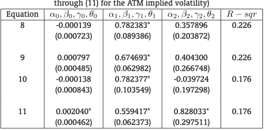
Table 2 presents the coefficient estimates for equations (8) through (11) using the ATM (at-the-money) estimation of implied volatilities (IV). The results are non-conclusive regarding the explana-tory power, i.e., they indicate that the explanaexplana-tory power of the implied volatilities are not super-seded by and do not supersede the standard deviation estimate’s or the conditional standard deviation TGARCH(1,1)’s.
Table 2 –Informational Content Analysis
(coefficients, standard errors and R-squared of equations (8) through (11) for the ATM implied volatility)
Equation α0, β0, γ0, θ0 α1, β1, γ1, θ1 α2, β2, γ2, θ2 R−sqr
8 -0.000139 0.782383* 0.357896 0.226
(0.000723) (0.089386) (0.203872)
9 0.000797 0.674693* 0.404300 0.226
(0.000485) (0.062982) (0.266748)
10 -0.000138 0.782377* -0.039724 0.176
(0.000843) (0.103549) (0.197298)
11 0.002040* 0.559417* 0.828033* 0.176
(0.000462) (0.062373) (0.297511)
Standard errors are shown in parenthesis.
Values with * represent significantly positive estimates at the 1% significance level.
Moreover, we aim to assess the informational content of implied volatilities based on Malz (2000) approach, which applies Granger causality test in order to capture lagged relationship higher than one-day length. Despite Granger causality does not provide a notion of causality in an economic sense,
12ˆǫT GARCH
t accounts for the TGARCH(1,1)-volatility’s movements not explained by the implied-volatility’s.
it may be very useful to indicate the lead-lag relationship between two variables. We determined maximum length of 10 business days and the optimal lag length is chosen by AIC (Akaike Information Criteria) using univariate VAR (Vector Auto Regressive) model. We obtained a lag equal to 8 business days for every regression, which is close to the lag of 5 arbitrarily chosen by Malz (2000), assuming that price adjustments occur within one trading week.
The Granger causality test basically verifies whether the conditional forecast variance of a depen-dent variable can be reduced significantly by including past information of another variable in the equation along lagged values of the dependent one itself. As shown in Greene (2003), tests comparing restricted and unrestricted equations can be based on a simple F test in the single equations of the VAR model.
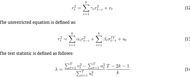
The restricted equation is defined as below, comprising only lagged values of the dependent vari-able. The use of squared returns, as proposed by Malz (2000), is intended to capture large magnitude returns, focusing on kurtosis rather than skewness of the return distribution:
r2
t = k
X
i=1
γir2t−i+vt (12)
The unrestricted equation is defined as:
r2
t = k
X
i=1
αir2t−i+ k
X
i=1
βiσIVt−i+ut (13)
The test statistic is defined as follows:
λ=
PT
t=1v 2
t−
PT
t=1u 2
t
PT
t=1u 2
t
T−2k−1
k (14)
whereutandνtare the residuals from the unrestricted and restricted regressions, respectively andTis
the sample size. The statisticλhas an asymptoticF(k, T−2k−1)distribution. If the critical value of the F distribution for a specified confidence level is lower thanλthe test will reject the null hypothesis stating that the new independent variable included in the unrestricted regression fails to Granger cause the dependent variable.
Table 3 contains the results for eq.(12) and eq.(13) comparison. In all the three cases, Granger causality is verified at a very low significance level, corroborating previous results on one-day ahead re-gressions which suggest that implied volatilities provide useful information on the prediction of future squared log-returns. The adjusted R-squared, also displayed in the table, indicate that previous squared returns in conjunction with implied volatilities estimates present significant explanatory power on fu-ture squared returns
Table 3 –Granger Causality Test for (12) and (13)
λ p-value R-sqr adj.
ATM 4.2 5.20E-05 0.229
GAMMA 3.3 1.10E-03 0.226
NT 3.1 1.85E-03 0.225
r2
t = k
X
i=1
αir2t−i+ k
X
i=1
βiσtT GARCH−i + k
X
i=1
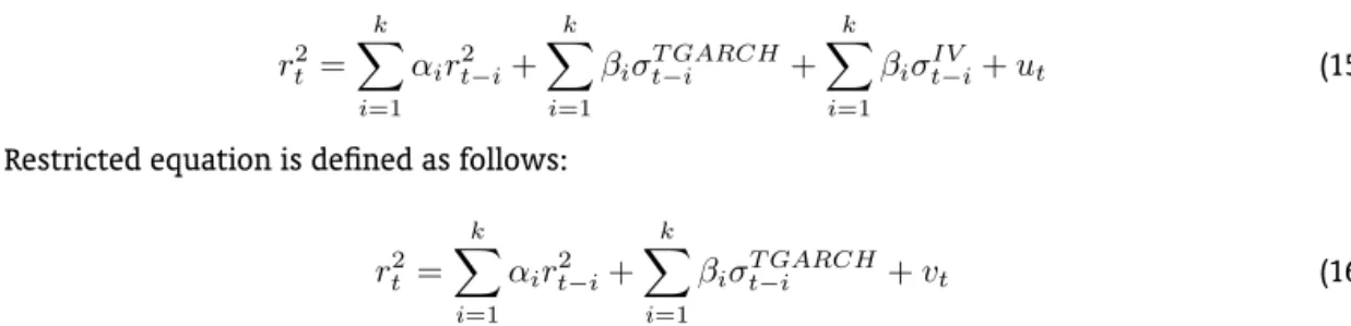
βiσIVt−i+ut (15)
Restricted equation is defined as follows:
r2
t = k
X
i=1
αirt2−i+ k
X
i=1
βiσtT GARCH−i +vt (16)
Table 4 contains the results for (15) and (16) comparison. Granger causality is also verified at a very low significance level, in line with previous results, corroborating that implied volatilities provide ad-ditional valuable information rather than time series estimates. The adjusted R-squared of unrestricted regressions indicates the significance of the variables and the expected increase in the explanatory power when compared to the above-mentioned results.
Table 4 –Granger Causality Test for (15) and (16)
λ p-value R-sqr adj.
ATM 4.3 3.40E-05 0.235
GAMMA 3.4 7.16E-04 0.233
NT 3.3 8.75E-04 0.232
3.2. Predictive Power
Initially, we applied the same approach used by Jorion (1995), in which the realized volatility is regressed against the ATM implied volatility (17) and against the average expected TGARCH(1,1) (18):
σt,T =δ0+δ1σtIV +ηt (17)
σt,T =θ0+θ1T GARCHt+νt (18)
where σt,T is the realized volatility betweentand the expiration date T, measured as the standard
deviation of daily returnsσIV,tis the implied volatility in date t for the period betweentandT and
T GARCHtis the average expected TGARCH(1,1).
To compute the forecast of the average conditional varianceT GARCH2
t, we followed the
deriva-tion in Heynen et al. (1994), which derives average expected GARCH(1,1) volatilities differing in times to maturity (see the Appendix A):
T GARCH2
t =
α0,t+1
1−αt+1−0,5γt+1−βt+1
+
ˆ
h2
t+1−
α0,t+1
1−αt+1−0,5γt+1−βt+1
(19)
1−(αt+1+ 0,5γt+1+βt+1)
τ
τ(1−αt+1−0,5γt+1−βt+1)
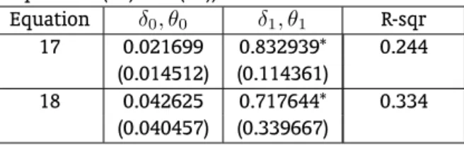
The forecasting series is then computed from the parameters estimation of the in-sample TGARCH(1,1) used in the previous section. The first lag of the explanatory variable is used as instrumental variable and the results of the GMM regressions (17) and (18) are presented in Table 5.
Table 5 –Predictive Power Analysis
(coefficients, standard errors and R-squared of equations (17) and (18))
Equation δ0, θ0 δ1, θ1 R-sqr
17 0.021699 0.832939* 0.244
(0.014512) (0.114361)
18 0.042625 0.717644* 0.334
(0.040457) (0.339667)
Standard errors are shown in parenthesis.
Values with * represent significantly positive estimates at the 1% sig-nificance level.
information content analysis. Now, the aim is to compare the predictive performance of the implied volatility only against TGARCH(1,1) taking the realized volatility as the dependent variable:
σt,T =α0+α1σtIV +α2ˆǫT GARCHt +ηt (20)
σt,T =γ0+γ1T GARCHt+γ2ˆǫIVt +νt (21)
where ˆǫT GARCH
t is the estimated residual of the GMM regression T GARCHt = δ0 +δ1σtIV +
ǫT GARCH
t andˆǫIVt is the estimated residual of the GMM regressionσIVt =λ0+λ1T GARCHt+ǫIVt .
We used the first lag of each explanatory variable as instrumental variables and the results of the GMM regressions (20) and (21) are presented in Table 6. The ATM implied volatility is found to be an efficient volatility predictor at the 5% significance level, i.e., one cannot reject that the ATM implied volatility may contain incremental information regarding the TGARCH(1,1), asα1and γ2are signifi-cantly different from zero at the 5% significance level, whilea2is non-significant.
Table 6 –Encompassing Test
(coefficients, standard errors and R-squared of equations (20) and (21))
Equation α0, γ0 α1, γ1 α2, γ2 R-sqr
20 0.021743 0.832898* 0.173603 0.299
(0.015561) (0.121484) (0.233193)
21 0.042688* 0.717452* 0.658898* 0.299 (0.014328) (0.120203) (0.250823)
Standard errors are shown in parenthesis.
Values with * represent significantly positive estimates at the 1% significance level. Values with ** represent significantly positive estimates at the 5% significance level.
3.3. Sub-sample Analysis
As a whole, the results did not change significantly. For the second sub-sample, which comprises more than a half of the entire sample, results are completely robust, as they lead to the same conclu-sions. The results for the first sub-sample, however, are not conclusive with regards to the predictive efficiency, i.e., one cannot affirm that the ATM implied volatility contains incremental information when compared to the TGARCH(1,1), and vice-versa.14
4. SIGNALING FOR TAIL EVENTS
In the previous sections we have shown that implied volatility on real-dollar options contains rel-evant information about future large-magnitude returns. From now on, our intention is to use this information to build a practical tool that may work as a warning system for stress events.
The goal here is to follow Malz (2000) and measure the probability of a week-ahead large movement in real-dollar exchange rate conditional to observedhighandrisingimplied volatility, and then verify whether or not there is independence between signal and future event.
The signaling tool consists, basically, of verifying the independence between two distinct events. The first one, which determines the subset of weeks A, is related to the occurrence ofhighandrising
implied volatility in the one week. Once it is verified the occurrence of this event, a signal is considered to have been sent. The second event, which determines the subset B, refers to the occurrence ofhigh
absolute returns of the underlying asset (real-dollar exchange rate) one week ahead.
Because of the results presented in the predictive power section, where ATM options implied volatili-ties are highly superior in terms of R-squared when compared to the other estimates of implied volatility, the signaling test is performed based only on the ATM estimate.
The signaling is tested always based on weekly data observed every Wednesday,15as suggested by
Malz (2000) in order to avoid the day-of-the-week bias. Therefore, to define ahighimplied volatility, a series of daily implied volatilities is used to calculate, for each day, the average and the standard devia-tion of the previous 252 observadevia-tions. If the estimate for a specific Wednesday is one standard deviadevia-tion higher than the average, both computed for that specific date, the implied volatility is considered to be
high.
To obtain arisingimplied volatility it was necessary to compute log variations of implied volatilities between Wednesdays. Those values are then compared to the product of 0.674516and the standard
devi-ation of last 252 daily implied volatility log varidevi-ations, scaled up to week dimension through the square root rule. This last standard deviation encompasses the concept of vol of vol (volatility of volatility), which in certain way reveals the magnitude of the variability of the daily implied volatility estimations in recent observations. If the implied volatility variation calculated from Wednesday to Wednesday is higher than this last product, it is considered to berising.
After that, weekly returns on the underlying asset, measured between Wednesdays, are considered to be high whenever its absolute value is higher than 2.33 (99th percentile) times the standard deviation of the last 252 daily log returns, scaled up into week dimension by the squared root rule.
Independence is verified through Chi-square and Fisher’s Exact tests based on the 2x2 contingency table presented below. Both of them tests for the null hypothesis of independence between events A and B. Therefore, the rejection of the null hypothesis lead to the interpretation that the implied volatility does provide a good warning signal for large magnitude returns.
The test statistic of the chi-square test has an asymptotic chi-square distribution with 1 degree of freedom and is obtained as follows:
14In our view, the lack of predictive efficiency in the first sub-period (from November 1999 to October 2002) may be due to a
market-learning process, as the floating exchange rate regime had been implemented a couple of months before (February 1999).
Table 7 –Signaling Test
Observed N(B) N(∼B) Total
N(A) 6 36 42
N(∼A) 10 339 349
Total 16 375 391
Observed values for subsets A and B, extracted from the implied volatilities on ATM real-dollar options. N(A) corresponds to the number of events of the subset A (implied volatility high and ris-ing). N(B) corresponds to the number of events of subset B (high returns). N(∼A) and N(∼B) are the denials of subsets A and B.
χ2
=
2 X
j=1 2 X
k=1
(Njk−Nj.NN.k)2 Nj.N.k
N
(22)
withNjkas the number of elements in thejkth cell and with the dots indicating totals of columns
and cells. The value for the above contingency table is 12.46, with an associated p-value of 0.042%, suggesting that implied volatility signals for real-dollar large magnitude returns at a 99.38% confidence level.
Fisher (1922) has shown that Chi-square test, due to its asymptotic feature, provides inaccurate results when the expected numbers for the contingency table are small. Alternatively, the author rec-ommends the application of a hypergeometric test, which p-value associated with the null hypothesis of independence is given by the following hypergeometric probability function:
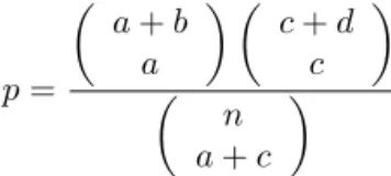
p=
a+b
a
c+d c
n a+c
(23)
Accordingly, as mentioned before, we have also performed the Fisher’s exact test for independence and with a p-value of 0.326% the test rejects the null hypothesis of independence at the 1% significance level.
Robustness is checked by varying the thresholds used to identifyhighreturns andhighand rising implied volatilities. Originally, Malz (2000) used 2.33 standard deviations forhighreturns, and 1.00 and 0.6745 standard deviations forhighandrisingimplied volatilities, respectively. Here, we use different thresholds ranging from 0.6745 to 2.33. Generally, the null hypothesis cannot be rejected whenever low thresholds (0.6745 and 1.00) are used to identifyhighreturns.
4.1. Controlling for Serial Correlation
Notwithstanding these results, we share Malz (2000) concerns that the tests performed earlier in this section have major limitations when applied to financial time series. Data sample frequency and volatility clustering, which are broadly acknowledged stylized facts for financial returns, may bias the sample or suggest for spurious relationship. Hence, although we interpret our results as strong evi-dence for market signaling, we understand that further development on the implementation of signal-ing tools in financial markets must be done.
week ahead. We understand that this modification can control for serial correlation in the sense that subsequent returns of the same magnitude will never represent a signaling event.
Risingreturns are those that present an absolute difference from last absolute return higher than 0.6745 multiplied by the standard deviation of the last 252 daily log returns, scaled-up to week dimen-sion through the square root rule. P-values obtained from the Chi-square and Fisher’s exact tests are 0.396% and 1.241%, respectively, corroborating previous results that implied volatility signals for large magnitude returns. Robustness is also checked as before and, overall, the null hypothesis cannot be rejected whenever very high thresholds (2.33) are used to identifyhighimplied volatilities.
5. CONCLUDING REMARKS
The purpose of the current work is to test one of the techniques created to obtain, from the informa-tion contained in financial asset prices, useful informainforma-tion about unusual future price movements. Its specific aim is to verify if real-dollar options’ implied volatilities can provide useful information about large-magnitude returns in the future. Besides testing this informational content, the implied volatili-ties’ predictive power is also checked. Finally, it is proposed, based on Malz (2000), a practical warning system to capture the informational content of implied volatilities in real-dollar options.
With regards to the informational content analysis, Granger causality is verified at a very low signif-icance level, corroborating previous results on one-day ahead regressions which suggests that implied volatilities provide useful information about large-magnitude returns in the future. In the case of the predictive power test, all implied volatilities measures are found to be efficient volatility predictors at the 1% significance level. This result demonstrates the capability of implied volatilities to predict future realized price variations on the underlying assets.
Finally, the signaling test indicates that the monitoring of implied volatilities on real-dollar options can be used to build an efficient and practical warning system for stress events in the future.
Bibliography
Ahoniemi, K. (2006). Modeling and forecasting implied volatility: An econometric analysis of the VIX index. Helsinki School of Economics, Discussion Paper 129.
Amin, K. & Jarrow, R. A. (1991). Pricing foreign currency options under stochastic interest rates.Journal of International Money and Finance, 10:310–329.
Andrade, S. C. & Tabak, B. M. (2001). Is it worth tracking dollar/real implied volatility? Revista de Economia Aplicada, 5(3).
Becker, J. L. & Lemgruber, E. F. (1989). Uma análise de estratégias de negociação no mercado brasileiro de opções: Evidências a partir das opções de compras mais negociadas durante o Plano Cruzado. In Brito, editor,Gestão de Investimentos. Editora Atlas.
Beckers, S. (1981). Standard deviations implied in options prices as predictors of future stock price volatility. Journal of Banking and Finance, 5:363–81.
Berg, A. & Pattillo, C. (1998). Are currency crises predictable? A test. IMF Working Paper Series. n. 98/154.
Black, F. (1976). The pricing of commodity contracts. Journal of Financial Economics, 4:167–179. Black, F. & Scholes, M. (1972). The valuation of option contracts and a test of market efficiency. Journal
Blejer, M. I. & Schumacher, L. (1998). Central bank vulnerability and the credibility of commitments: A value-at-risk approach to currency crises. IMF Working Paper Series, N. 98/65.
Breeden, D. T. & Litzenberger, R. H. (1978). Prices of state contingent claims implicit in option prices.
Journal of Business, 51:621–652.
Castro, P. C. (2002). Opções sobre dólar comercial e expectativas a respeito do comportamento da taxa de câmbio. Banco Central do Brasil, Brasília.
Chesney Marc, S. L. (1989). Pricing european currency options: A comparison of the modified Black-Scholes model and a random variance model.Journal of Financial and Quantitative Analysis.
Christensen, B. & Prabhala, N. R. J. (1998). The relation between implied and realized volatility. Journal of Financial Economics, 50(3):125–150.
Craig, B. R. & Keller, J. G. (2004). The forecast ability of risk-neutral densities of foreign exchange. Federal Reserve Bank of Cleveland, WP 04-09.
Cunha Jr., D. & Lemgruber, E. F. (2003). Opções de dólar no brasil com taxas de juro e de cupom estocás-ticos. III Encontro Brasileiro de Finanças. FEA, USP.
Da Costa, M. N. & Yoshino, J. A. (2004). Calibração do modelo de heston para o mercado brasileiro. IV Encontro Brasileiro de Finanças.
Day, T. & Lewis, C. (1992). Stock market volatility and the information content of stock index options.
Journal of Econometrics, 52:267–287.
Dickey, D. A. & Fuller, W. A. (1979). Distribution of the estimators for autoregressive time series with a unit root. Journal of the American Statistical Association, 74:427–431.
Doran, J. S. & Ronn, E. I. (2006). The bias in Black-Scholes/Black implied volatility: An analysis of equity and energy markets. Florida State University Working Paper.
Duan, J. (1995). The GARCH option pricing model. Mathematical Finance, 5(1):13–32.
Feiger, G. & Jacquillat, B. (1979). Currency option bonds, puts and calls on spot exchange and the hedging of contingent foreign earnings.Journal of Finance, 34:1129–139.
Fisher, R. A. (1922). On the interpretation ofχ2
from contingency tables, and the calculation of P.Journal of the Royal Statistical Society, 85(1):87–94.
Frankel, J. A. & Rose, A. K. (1996). Currency crashes in emerging markets: An empirical treatment.
Journal of International Economics, 41:351–366.
Garman, M. & Kohlhagen, S. (1983). Foreign currency options values.Journal of International Money and Finance, 2:231–237.
Glosten, L. R., Jagannathan, R., & Runkle, D. (1993). On the relation between the expected value and the volatility of the nominal excess return on stocks. Journal of Finance, 48:1779–1801.
Gomes, F. P. (2002). Volatilidade implícita antecipada de eventos de stress: Um teste para o mercado brasileiro. Departamento de Estudos e Pesquisas, Banco Central do Brasil, Brasília.
Granger, C. W. J. (1969). Investigating causal relations by econometric methods and cross-spectral meth-ods. Econometrica, 34:424–438.
Greene, W. H. (2003). Econometric Analysis. Prentice Hall, 5th edition.
Heston, S. (1993). A closed-form solution for options with stochastic volatility with applications to bond and currency options. The Review of Financial Studies, 6(2).
Heynen, R., Kemna, A., & Vorst, T. (1994). Analysis of the term structure of implies volatilities. Journal of Financial Quantitative Analysis, 29:31–46.
Hilliard, J. E., Madura, J., & Tucker, A. L. (1991). Currency option pricing with stochastic domestic and foreign interest rates. Journal of Financial and Quantitative Analysis, 26(2):139–151.
Hull, J. (2003). Options, Futures and Other Derivatives Securities. Prentice Hall, New Jersey, 5 edition. Hull, J. & White, A. (1987). The pricing of options on assets with stochastic volatilities.Journal of Finance,
42:281–300.
Jorion, P. (1995). Predicting volatility in the foreign exchange market. The Journal of Finance, 50(2):507– 528.
Kaminsky, G., Lizondo, S., & Reinhart, C. (1998). Leading indicators of currency crises. IMF Staff Papers, 45(1):01–48.
Lemgruber, E. F. (1995). Avaliação de Contratos de Opções. BM&F, São Paulo, revisada e ampliada edition. Malz, A. M. (2000). Do implied volatilities provide early warning of market stress? RiskMetrics Journal,
1(1):41–60.
Matos, J. A., Kapotas, J. C., & Schirmer, P. P. (2004). Pricing and hedging brazilian currency options. IV EBF.
Melino, A. & Turnbull, S. M. (1991). The pricing of foreign currency options. Canadian Journal of Eco-nomics, Canadian Economics Association, 24(2):251–81.
Merton, R. (1973). Theory of rational option pricing. Bell Journal of Economics, 4:141–183.
Navatte, P. & Villa, C. (2000). The information content of implied volatility, skewness and kurtosis: Empirical evidence from long-term CAC 40 options. European Financial Management, 6(1):41–56. Neeley, C. (2004). Forecasting foreign exchange volatility: Why is implied volatility biased and
ineffi-cient? And does it matter? Federal Reserve Bank of St. Louis Working Paper.
Pownall, R. A. J. & Koedijk, K. G. (1999). Capturing downside risk in financial markets: The case of the Asian crisis. Journal of Interantional Money and Finance, 18:853–870.
Scott, L. (1992). The information content of prices in derivative security markets. IMF Staff Papers, 39:596–625.
Scott, L. O. (1987). Option pricing when the variance changes randomly: Theory, estimators, and appli-cations. Journal of Finance and Quantitative Analysis, 22:419–438.
Scott, L. O. (1991). Random variance option pricing.Advances in Futures and Options Research, 5:113–135. Stein, E. M. & Stein, J. C. (1991). Stock price distributions with stochastic volatility.The Review of Financial
Vasicek, O. (1977). An equilibrium characterization of the term structure.Journal of Financial Economics, 5:177–188.
Wiggins, J. (1987). Option values under stochastic volatility: Theory and empirical estimates.Journal of Financial Economics, 19:351–372.
APPENDIX A
Following Heynen et al. (1994) we derive the formula of the average expected volatility for the TGARCH (1,1) volatility stochastic process, as follows:
Rt=C+µRt−1+ǫt
h2
t =α0,t+ (αt+γtIt)ǫ2t−1+βt.h
2
t−1 where:
Rtis the daily log-return;
ǫt∼N(0, h2t), and;
It= 0, ǫt≥0
1, ǫt<0 .
The average expected volatility betweentandt+kis defined as:
T GARCH2
(t, t+k) = 1
T
k
X
t=1
Eth2t+k
Firstly, it is necessary to expressht+kin terms ofht. We start by:
h2
t+k=α0,t+ (αt+γtIt+k−1)ǫ
2
t+k−1+βth
2
t+k−1
From Glosten et al. (1993) we have that the condictional variance, at datet,k-days ahead, assuming
P(ǫt>0) = 50%, is computed as:
E h2
t+k
=h2
+ (αt+ 0,5γ+βt)k−1 h2t+1−h
2
where the inconditional (long-run) variance is defined as:
h2
=α0,t (1−αt−0,5γt−βt)−
1
As the formula of the average expected volatility contains a geometruic series, we use the formula of the sum of the terms of the geometric progression and express the average express volatility as:
T GARCH2
(t, t+k) = 1
k (
kh2
+ h2
t+1−h
2(αt+ 0,5γt+βt)
k
−1
αt+ 0,5γt+βt−1
)
withλ= (αt+ 0,5γt+βt), we finally have:
T GARCH2
(t, t+k) =h2
+1
k
h2
t+1−h 2λ
k
−1
λ−1
whereσ2